Modification of late time phase structure by quantum quenches

Abstract

The consequences of the sudden change in the coupling constants (quenches) on the phase structure of the theory at late times are explored. We study in detail the three dimensional $\phi^{6}$ model in the large $N$ limit, and show that the $\phi^{6}$ coupling enjoys a widened range of stability compared to the static scenario. Moreover, a new massive phase emerges, which for sufficiently large coupling becomes the dominant vacuum. We argue that these novel phenomena cannot be described by a simple thermalization effect or the emergence of a single effective temperature.

1 Introduction

Unlocking the problem of out-of-equilibrium dynamics of a quantum coherent system is one of the fundamental questions in quantum phyiscs. This is particularly true in the context of quantum field theories, where many important questions have so far been addressed mainly in a static scenario, such as the renormalization group flow, the phase structure of vacuua and critical points. There are also interesting questions that spring directly from a non-equilibrium system, such as the mechanisms of relaxation, the time-scale over which this occurs, and the existence of an effective description at late times. These problems, given their fundamental role in field theories, naturally appear in many places. For example, it is not surprising that non-equilibrium dynamics are important in cosmology, in the evolution of the early universe. The RHIC experiments, involving the relaxation of the quark-gluon plasma, is another such example. Dynamical systems appear frequently in the context of condensed matter physics. Recently, the study has been rendered particularly pertinent experimentally due to new advances in the control of cold atomic gasesrelax ; relax1 ; relax2 ; Newcrad . For the first time, we are able to observe minute details of the evolution of a system that retains its quantum coherence for sufficiently long periods of time. One class of situations that has been subjected to intensive studies is called the quantum quench, in which a particular external field, or parameter, of the system is changed abruptly. An example is a sudden change of the external magnetic field to which the atoms couple. These experiments have inspired a flurry of theoretical activities, most notably initiated by Calabrese and Cardy cardyquench . Previous works however, have been concentrated on free field theories, one-dimensional interacting theories and integrable models, see e.g. oned1 ; oned2 ; oned3 ; oned4 ; rigol ; CEF ; caneva Attempts to understand interacting theories in higher dimensions by considering the large $N$ limit of a $\phi^{4}$ theory have been made in Sotiriadis:2010si .(See also the related problem Das:2012mt ).

Previous studies of the quenches concerned mostly about the relaxation of the system. One central issue is whether the system thermalizes and therefore describable by an effective temperature at late times. It is however an open problem if thermalization occurs at all, and if it does not, which is shown to be the case in many integrable models and in some cases even interacting models (see for example rigol ), whether there are convenient effective descriptions of such systems and observables or effective parameters that characterize their behavior. This leads us to the current investigation of the phase structure of some out-of-equilibrium state, which in the scenario concerned is prepared by a quantum quench. This should be contrasted with the usual notion of the phase structure of a given Hamiltonian, which is a property of its ground state. Here, we have to deal with a state, which, while settling to some static equilibrium in the far future, does not resemble a thermal state, nor is it able to relax to the ground state because of its isolation and energy conservation after the quench. It is therefore only natural to consider fluctuations about such a special state as oppose to the ground state, and determine its corresponding phase structure.

In this work, we demonstrate that this phase structure differs significantly from that of the ground state even at late times as the system approaches equilibrium again.

In particular, we explore the $g_{6}\phi^{6}$ theory at the tricritical point, i.e., when all dimensionful couplings except the physical mass immediately after the quench are tuned to zero. What is special about this model is that it was shown to possess an ultraviolet fixed point $g_{6}=192$ using the $1/N$ expansion about $N=\infty$ Townsend:1975kh ; Pisarski:1982vz . This fixed point however lies in the instability region of the model where the non-perturbative effects dominate Bardeen:1983rv . The latter implies that the theory is always driven into the unstable region by the $\beta$-function and therefore apparently does not make physical sense. We revisit this theory in the context of quantum quenches. To that end, we employ the methods introduced in Sotiriadis:2010si , where the effect of a quench is incorporated as a boundary condition on the fields. Assuming that the system does settle down, we then self-consistently compute the effective potential which defines the notion of phase structure of the theory at late times. We thus obtain a corresponding phase diagram, which surprisingly is modified dramatically in comparison to the unquenched case. The region of stability is substantially widened such that the UV fixed point of the $\beta$-function now lies well within. Moreover, a new stable minimum in the effective potential emerges when the coupling constant exceeds the upper bound of the stability range in the static theory. The new vacuum starts life as a meta-stable phase, but then becomes dominant for sufficiently large values of the coupling. In particular, the effective mass of the new phase increases as the coupling increases, and eventually diverges when the coupling hits the boundary of a newly established range of stability.

In the following, we will employ large $N$ expansion and study in detail the quench dynamics of the massive scalar $O(N)$ vector model.

2 Quenching the scalar model

The scalar $O(N)$ vector model consists an $N$-component scalar field $\phi$. For simplicity we assume that initially the theory is free and the system is prepared in the ground state of a free hamiltonian $|\Psi_{0}\rangle$. At $t=0$ the marginal $\phi^{6}$ interaction as well as relevant $\phi^{4}$ interaction are instantaneously switched on, and at the same instant the bare mass parameter of the field jumps from $\mu_{0}$ to $\mu$. The action of the system after the quench is given by

$$S(\phi)={1\over 2}\int d^{3}x\big{[}{\partial}_{\mu}\phi{\partial}^{\mu}\phi-\mu^{2}\phi^{2}-{g_{4}\over 2N}(\phi^{2})^{2}-{g_{6}\over 3N^{2}}(\phi^{2})^{3}\big{]}~{}.$$ (1)

Since parameters of the theory are changed abruptly rather than adiabatically, one needs to resort to the well-known Keldysh-Schwinger, or in-in, formalism for non-equilibrium quantum systems. In this formalism the integration over time coordinate $t$ in the path integral starts from some initial time $t_{i}$, extends to some final time $t_{f}$ and then goes back to $t_{i}$. Correlation functions are path ordered. In this approach one needs to impose boundary conditions at $t=t_{i}$. In our case we impose that the initial state at $t_{i}=0$ is given by $|\Psi_{0}\rangle$.

The expectation value of an arbitrary operator $\mathcal{\hat{O}}(t)$ is given by

$$\langle\Psi_{0}|\mathcal{\hat{O}}(t)|\Psi_{0}\rangle=\int_{CTP}D\phi\,\mathcal{\hat{O}}(t)\,e^{iS(\phi)}~{},$$ (2)

where for brevity we use the following notation to designate the closed-time-path (CTP) integral measure

$$\int_{CTP}D\phi=\int D\phi_{i}\,\Psi_{0}(\phi_{i})\int D\tilde{\phi}_{i}\,\Psi_{0}^{*}(\tilde{\phi}_{i})\int_{\phi_{i}}^{\tilde{\phi}_{i}}D\phi~{},$$ (3)

where $\phi_{i}$ and $\tilde{\phi}_{i}$ denote the values of the scalar field $\phi$ at the end points of the time contour, whereas $\Psi_{0}(\phi_{i})=\langle\phi_{i}|\Psi_{0}\rangle$ and similarly for the complex conjugate $\Psi_{0}^{*}(\tilde{\phi}_{i})$.

Introducing the following identity into the path integral

$$\mathbb{I}\sim\int_{CTP}D\rho\,\delta(\phi^{2}-N\rho)\sim\int_{CTP}D\rho D\lambda~{}e^{-{i\over 2}\int d^{3}x\,\lambda(\phi^{2}-N\rho)}~{},$$ (4)

yields

$$\langle\Psi_{0}|\mathcal{\hat{O}}(t)|\Psi_{0}\rangle=\int_{CTP}D\phi\int D\rho D\lambda\,\mathcal{\hat{O}}(t)\,e^{iS(\phi,\rho,\lambda)}~{},$$ (5)

where

$$S(\phi,\rho,\lambda)={1\over 2}\int d^{3}x\big{[}{\partial}_{\mu}\phi{\partial}^{\mu}\phi-(\mu^{2}+\lambda)\phi^{2}-N{g_{4}\rho^{2}\over 2}-N{g_{6}\rho^{3}\over 3}+N\rho\lambda\big{]}~{}.$$ (6)

Performing now the Gaussian integral over $\phi$ leads to

$$\langle\Psi_{0}|\mathcal{\hat{O}}(t)|\Psi_{0}\rangle=\int_{CTP}D\rho D\lambda\,\mathcal{\hat{O}}(t)\,e^{iNS_{eff}(\rho,\lambda)}~{},$$ (7)

with

$$S_{eff}(\rho,\lambda)=\int d^{3}x\left[{\lambda\,\rho\over 2}-{g_{4}\over 4}\rho^{2}-{g_{6}\over 6}\rho^{3}\right]+{i\over 2}\text{Tr}\log(\square+\mu^{2}+\lambda)~{}.$$ (8)

The first thing to note about the above expression is that boundary conditions are now encoded in the functional trace. Secondly, this trace explicitly depends on the integration parameter $\lambda$, and this in turn renders evaluation of the remaining path integral very difficult.

However, in the limit when $N$ is large while $g_{4}$ and $g_{6}$ are fixed, the right hand side of (7) is dominated by the field configurations which minimize (8), i.e., solutions of the corresponding classical equations of motion. The effective mass can thus be evaluated. This is often called the stationary phase approximation. This gives

$$m_{\phi}^{2} = \mu^{2}+g_{4}\bar{\rho}+g_{6}\bar{\rho}^{2}~{},$$

$$\bar{\rho} = \int{d^{2}p\over(2\pi)^{2}}\,\tilde{G}_{\phi}(t,t;p)~{},$$ (9)

where $m_{\phi}^{2}=\mu^{2}+\bar{\lambda}$ is the effective mass of the scalar field and $\tilde{G}_{\phi}(t_{1},t_{2};p)$ is the full momentum space two point correlation function of the scalar field to leading order in $1/N$. Fields evaluated at the saddle point are denoted by a bar.

Note that $\tilde{G}_{\phi}(t_{1},t_{2};p)$ depends on the effective mass $m_{\phi}^{2}$, and therefore it is difficult to solve (9) in full generality. Hence, in what follows we use the approximation proposed in Sotiriadis:2010si . In particular, we assume that $m_{\phi}$ tends to a stationary value $m_{\phi}^{*}$ and that this happens fast enough to be approximated by a jump. Then the two point correlation function $\tilde{G}_{\phi}(t_{1},t_{2};p)$ is approximately the same as the propagator in the massive free field theory in which the physical mass is instantaneously changed from $\mu_{0}$ to $m_{\phi}^{*}$. i.e.,

$$\tilde{G}_{\phi}(t_{1},t_{2};p)\simeq G_{\phi}(t_{1},t_{2};p;\mu_{0},m^{*}_{\phi})~{},$$ (10)

where Sotiriadis:2010si

$$G_{\phi}(t_{1},t_{2};p;\mu_{0},m^{*}_{\phi})={(\omega_{p}^{*}-\omega_{0p})^{2}\over 4\omega_{p}^{*2}\omega_{0p}}\cos\omega_{p}^{*}(t_{1}-t_{2})+{\omega_{p}^{*2}-\omega_{0p}^{2}\over 4\omega_{p}^{*2}\omega_{0p}}\cos\omega_{p}^{*}(t_{1}+t_{2})+{1\over 2\omega_{p}^{*}}e^{-i\omega_{p}^{*}|t_{1}-t_{2}|}~{},$$ (11)

with $\omega_{p}^{*}=\sqrt{\vec{p}^{\,2}+m_{\phi}^{*2}}$ and $\omega_{0p}=\sqrt{\vec{p}^{\,2}+\mu_{0}^{2}}$. The second term on the right hand side is the only one that breaks time translation invariance. However, its contribution to $\bar{\rho}$ vanishes for $t_{1}=t_{2}=t\rightarrow\infty$ within our stationary phase approximation. Therefore (9) yields the following equation for $m^{*}_{\phi}$

$$m_{\phi}^{*2}=\mu^{2}-{g_{4}\over 4\pi}\bigg{(}\mu_{0}+{1\over 2}\sqrt{m_{\phi}^{*2}-\mu_{0}^{2}}\,\arccos\bigg{(}{\mu_{0}\over m_{\phi}^{*}}\bigg{)}-\Lambda\bigg{)}\\ +{g_{6}\over 16\pi^{2}}\bigg{(}\mu_{0}+{1\over 2}\sqrt{m_{\phi}^{*2}-\mu_{0}^{2}}\,\arccos\bigg{(}{\mu_{0}\over m_{\phi}^{*}}\bigg{)}-\Lambda\bigg{)}^{2}~{},$$ (12)

where we have taken a sharp cut off $\Lambda$ to regulate the divergent integral over the momentum. To eliminate the cut off dependence we apply the following renormalization scheme

$$\mu_{R}^{2} = \mu^{2}+{g_{4}\over 4\pi}\Lambda+{g_{6}\over 16\pi^{2}}\Lambda^{2}~{},$$

$$g_{4}^{R} = g_{4}+{g_{6}\over 2\pi}\Lambda~{}.$$ (13)

As a result, the gap equation for $m^{*}_{\phi}$ becomes

$$m_{\phi}^{*2}=\mu^{2}_{R}-{g_{4}^{R}\over 4\pi}\bigg{(}\mu_{0}+{1\over 2}\sqrt{m_{\phi}^{*2}-\mu_{0}^{2}}\,\arccos(\mu_{0}/m_{\phi}^{*})\bigg{)}\\ +{g_{6}\over 16\pi^{2}}\bigg{(}\mu_{0}+{1\over 2}\sqrt{m_{\phi}^{*2}-\mu_{0}^{2}}\,\arccos(\mu_{0}/m_{\phi}^{*})\bigg{)}^{2}~{}.$$ (14)

Solutions of this gap equation describe the stationary points of the effective potential. In the following we analyze these solutions and demonstrate that the quenched model exhibits peculiar phase structures.

3 Phase structure of the model

To analyze the admissible phases of the model let us derive the effective potential of the theory at $t\rightarrow\infty$. From (8), we get, up to $\bar{\lambda}$-independent constant,

$$V_{eff}(\bar{\rho},m_{\phi}^{*2})={\mu^{2}\over 2}\bar{\rho}+{g_{4}\over 4}\bar{\rho}^{2}+{g_{6}\over 6}\bar{\rho}^{3}-{m_{\phi}^{*2}\,\bar{\rho}\over 2}+{1\over 2}\int_{0}^{m_{\phi}^{*2}}dm^{2}\int^{\Lambda}{d^{2}p\over(2\pi)^{2}}\,G_{\phi}(t,t;p;\mu_{0},m)~{}.$$ (15)

Varying this effective potential with respect to $\bar{\rho}$ and $m_{\phi}^{*2}$ correctly reproduces the saddle point equations (9). Note that $\rho$ is not a dynamical field since it enters only algebraically into the action (8). Hence we eliminate it from the effective potential using the second equation (9). Replacing the couplings by renormalized ones and further rescaling them by $\mu_{0}$ yields

$$\tilde{V}_{eff}(m^{2})=-{\tilde{\mu}_{R}^{2}\over 8\pi}\bigg{(}1+{1\over 2}\sqrt{m^{2}-1}\,\arccos(1/\sqrt{m^{2}})\bigg{)}\\ +{\tilde{g}_{4}^{R}\over 4(4\pi)^{2}}\bigg{(}1+{1\over 2}\sqrt{m^{2}-1}\,\arccos(1/\sqrt{m^{2}})\bigg{)}^{2}\\ -{g_{6}\over 6(4\pi)^{3}}\bigg{(}1+{1\over 2}\sqrt{m^{2}-1}\,\arccos(1/\sqrt{m^{2}})\bigg{)}^{3}\\ +{(m^{2}+2)\sqrt{m^{2}-1}\arccos(1/\sqrt{m^{2}})+m^{2}-\log m^{2}\over 48\pi}~{},$$ (16)

where $\tilde{V}_{eff},\,\tilde{\mu}_{R},\,\tilde{g}_{4}^{R}$ and $m^{2}$ denote respectively the rescaled dimensionless effective potential, the dimensionless renormalized couplings and asymptotic mass.

Let us briefly discuss the case where both $g_{6}$ and $\mu_{R}$ are zero. This case was considered in Sotiriadis:2010si . The characteristic shape of the effective potential of the quenched theory in this case is shown in figure 1(red line), and as pointed out in Sotiriadis:2010si a finite mass always emerges at late times in the presence of interactions. This should be contrasted with the presence of a global minimum at $m=0$ in the unquenched theory as shown in figure 1(blue line).

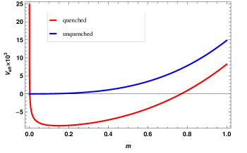
Figure 1: Red line (bottom): effective potential (16) as a function of $m$ for $g_{6}=\mu_{R}=0$ and $\tilde{g}_{4}^{R}=1$.
Blue line (top): effective potential of the $\phi^{4}$ theory, i.e., $g_{6}=0$, in the absence of quench when $\mu_{R}=0$ and $\tilde{g}_{4}^{R}=1$.

This case already illustrates the main point that we wish to make, namely that the shape of the effective potential at late times depends on the quench, an event that occurred in the far past. More interesting and spectacular however is the case when the theory is sitting at the tricritical point, i.e., when $\mu_{R}=g_{4}^{R}=0$. Expanding effective potential then for large and small values of $m^{2}$ yields

$$\tilde{V}_{eff}(m) = {m^{3}\over 96}\bigg{(}1-{g_{6}\over g_{c}}\bigg{)}+\mathcal{O}(m)\quad\quad\text{if}\quad m>>1~{},$$

$$\tilde{V}_{eff}(m) = -{g_{6}\over g_{c}}{\log^{3}m\over 12\pi^{3}}+\mathcal{O}(1)~{}\quad\quad\quad\text{if}\ \quad m<<1~{}.$$ (17)

where $g_{c}=256$ corresponds to a critical value beyond which the potential is unbounded from below and thus the theory is unstable.

It is remarkable that $g_{c}$ is larger than the corresponding value in the unquenched case Bardeen:1983rv . There, the region of stability is bounded by $0\leq g_{6}\leq(4\pi)^{2}\equiv g_{6}^{*}$. In particular, previous studiesTownsend:1975kh ; Pisarski:1982vz ; Bardeen:1983rv have spelled disaster for the theory in the ultraviolet limit: the $\beta$-function drives the system into a UV fixed point $g_{6}=192$ which lies beyond the region of stability. In contrast, our results indicate that there is a way to circumvent the above conclusion by a quench in the parameters of the system.

It is instructive to contrast the phase diagrams with those of the unquenched case. If the coupling constant belongs to the range $0\leq g_{6}<(4\pi)^{2}$ and the system is not quenched, then there is only one admissible conformal phase. Quenching the system in this regime, we explicitly break the conformal invariance by introducing a scale $\mu_{0}$, and as a result the system resides in the light phase - a unique vacuum state associated with the minimum of effective potential, see solid blue graph at the top of figure 2 which represents a characteristic plot of the effective potential in this case.

On the other hand, if the coupling constant is tuned to the special value $g_{6}^{*}$ the unquenched potential becomes flat, and thus a continuum of massive solutions emerges. This continuum is associated with spontaneous breaking of scale invariance and it coexists with the conformal (or massless) phase which we analyzed before. Quenching the system breaks the scale invariance explicitly and $\mu_{0}$ singles out a unique vacuum out of the continuum of states. As a result, in the steady state as $t\rightarrow\infty$ we find two admissible vacua shown in figure 2. The heavier phase for this value of the coupling is only meta-stable unless the coupling constant is sufficiently large, see dashed green and solid black graphs at the bottom of figure 2.

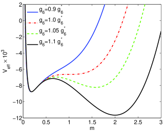
Figure 2: Effective potential (16) as a function of $m$ at the tricritical point $\mu_{R}=g_{4}^{R}=0$ in the vicinity of $g_{6}^{*}=(4\pi)^{2}$.

Of course, in the unquenched case all phases become unstable for $g_{6}>g_{6}^{*}$ and the system rolls down to infinity in a finite time Asnin:2009bs . Here we have showed how the quantum quench may enhance the stability of the system such that for $g_{6}>g_{6}^{*}$ these phases are stable and the escape to infinity is avoided until $g_{6}$ hits $g_{c}$.

4 Concluding remarks.

To conclude, by studying the late time phase structure of the $\phi^{6}$ theory after a quantum quench, we have essentially demonstrated in a specific example the following: a dramatic event that occurred in the far past can have significant effects even in the far future. Not entirely unexpectedly, we find that in the large $N$ limit the late time physics cannot be described by simple thermalization with a single effective temperature, which has been noted in many integrable models. Explicit details are relegated to Appendix A. Instead of simply thermalizing, the quantum quench appears to modify the phase structure, even long after the system has relaxed and settled into an equilibrium state. From the calculations, it appears that this is a generic feature of quantum quenches, and is not specific to the model that we have studied. In passing, we note also significant modifications in a supersymmetric version of this model: contrary to the current model, where new stable phases are created, we found instability generated by the quench inprogress . This dependence of the phase structure on past events may have implications in other areas of physics, e.g. in cosmology. It is therefore important to determine and perhaps classify, different time dependent changes in a generic theory that could potentially lead to drastic modification of late time physics.. In this work we have made extensive use of techniques developed in Sotiriadis:2010si , where it is implicitly assumed that the system relaxes ultimately to an equilibrium. The authors of Sotiriadis:2010si support their claim by explicit numerical computations and show that their assumption works very well in $\phi^{4}$ theories in arbitrary dimensions. In this work we extrapolate their assumption to study the $\phi^{6}$ theory at the tricritical point. Further numerical checks of the current model and more general ones are under way and will appear elsewhere inprogress .

Appendix A Absence of thermalization:

A question regarding the late time behavior studied in this work is whether it is effectively thermal. However, despite carrying interaction terms, the model we are studying is in fact integrable in the large $N$ approximation, and as noted in previous works, is not expected to be describable by a single effective temperature conjecture . In the rest of this appendix we demonstrate that the late time physics of our large $N$ vector model is incompatible with simple thermalization leading to a single effective temperature.

If the stationary behavior of the system is thermal, i.e., the effective mass $m_{\phi}^{*}$ is the thermal mass $m_{T}$ of the system. One can fix the temperature by matching the gap equation (9) at $t\rightarrow\infty$ with that in the thermal case. As a result, one gets the following relation which determines the inverse temperature $\beta$

$$\langle\phi^{2}\rangle_{0}=\langle\phi^{2}\rangle_{\beta}~{},$$ (18)

where subscripts “$\beta$” and “$0$” indicate that the expectation values are taken in the thermal and $|\Psi_{0}\rangle$ states respectively.

Having fixed the temperature via (18) (implicitly), we would like to compare the expectation value of the stress tensor of the thermal state with our quenched state at late times. The energy-momentum tensor of the scalar $O(N)$ vector model in Minkowski signature is given by

$$T_{\mu\nu}={\partial}_{\mu}\phi\cdot{\partial}_{\nu}\phi-\eta_{\mu\nu}\bigg{(}{1\over 2}{\partial}_{\mu}\phi\cdot{\partial}^{\mu}\phi-NV(\phi^{2}/N)\bigg{)}-{1\over 8}({\partial}_{\mu}{\partial}_{\nu}-\eta_{\mu\nu}{\partial}^{2})\phi^{2}~{}.$$ (19)

where $V(\phi^{2}/N)$ is the potential. The Euclidean form $T_{\mu\nu}^{E}$ is obtained by flipping the sign of the potential and replacing $\eta_{\mu\nu}$ with $\delta_{\mu\nu}$ in the above expression. In the large $N$ limit the expectation value $\langle V(\phi^{2}/N)\rangle$ equals $V(\langle\phi^{2}\rangle/N)$. Hence, provided that (18) holds, we get in the limit $t\rightarrow\infty$

$$\langle T_{00}\rangle_{0}+\langle T_{00}^{E}\rangle_{T}=\bigg{(}\eta_{0\alpha}\eta_{0\beta}-{1\over 2}\eta_{\alpha\beta}\bigg{)}\langle{\partial}^{\alpha}\phi\cdot{\partial}^{\beta}\phi\rangle_{0}+\bigg{(}\delta_{0\alpha}\delta_{0\beta}-{1\over 2}\delta_{\alpha\beta}\bigg{)}\langle{\partial}^{\alpha}\phi\cdot{\partial}^{\beta}\phi\rangle_{\beta}~{}.$$ (20)

The left hand side of the above expression should vanish if the system thermalizes since the zero-zero component of the Euclidean energy-momentum tensor is the minus energy density. Consider adding $m^{*2}_{\phi}\phi^{2}/2$ to the first term on the right hand side. We immediately identify that as $\langle T_{00}\rangle_{0}$ of a quenched free scalar field whose mass jumps from $\mu_{0}$ to $m^{*}_{\phi}$. On the other hand, subtracting $m^{*2}_{\phi}\phi^{2}/2$ from the second term gives the minus thermal energy of the free scalar field with mass $m_{\phi}^{*}$. Since the free theory does not thermalize, there is no temperature such that these two terms cancel each other. This proves a mismatch between thermal and quenched physics.

It is also instructive to compare the thermal free energy of the system at the tricritical point with the corresponding effective potential (16). In the large $N$ limit the thermal free energy density $f$ can be evaluated in a closed form and is given by

$$f/N={g_{6}\over 6}\left({m_{T}\over 4\pi}+{\log(1-e^{-\beta m_{T}})\over 2\pi\beta}\right)^{3}-{m_{T}^{3}\over 24\pi}-{m_{T}^{2}\log(1-e^{-\beta m_{T}})\over 4\pi\beta}\\ +\int_{0}^{m_{T}^{2}}{\log(1-e^{-\beta m_{T}})\over 4\pi\beta}dm_{T}^{2}~{}.$$ (21)

The typical plots are shown in figure 3. While for $g_{6}<g_{6}^{*}$ the free energy exhibits certain similarity with the corresponding effective potential, they become manifestly different for $g_{6}>g_{6}^{*}$ and hence thermalization is not expected.

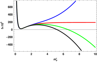
Figure 3: The plot of the free energy density $f$ for various values of the coupling constant $g_{6}$ as a function of effective mass $m_{\phi}^{*}$. $N=1$, the inverse temperature is set to $\beta=1$ and $g_{6}=0.9g_{6}^{*},~{}g_{6}^{*},~{}1.05g_{6}^{*},~{}1.1g_{6}^{*}$ from top to bottom graph respectively.

- (1) M. Greiner, O. Mandel, T. W. Haensch, and I. Bloch, Collapse and revival of the matter wave field of a bose-einstein condensate., Nature 419 (2002), no. 6902 51–54.
- (2) S. Hofferberth, I. Lesanovsky, B. Fischer, T. Schumm, and J. Schmiedmayer, Non-equilibrium coherence dynamics in one-dimensional bose gases., Nature 449 (2007), no. 7160 324–327.
- (3) S. Trotzky, Y.-A. Chen, A. Flesch, I. P. McCulloch, U. Schollw ck, J. Eisert, and I. Bloch, Probing the relaxation towards equilibrium in an isolated strongly correlated 1d bose gas, Physics 1101.2659 (2011) 8.
- (4) T. Kinoshita, T. Wenger, and D. S. Weiss, A quantum newton’s cradle., Nature 440 (2006), no. 7086 900–903.
- (5) P. Calabrese and J. Cardy, Time dependence of correlation functions following a quantum quench., Physical Review Letters 96 (2006), no. 13 136801.
- (6) M. A. Cazalilla, Effect of suddenly turning on interactions in the luttinger model., Physical Review Letters 97 (2006), no. 15 156403.
- (7) G. Roux, Quenches in quantum many-body systems: One-dimensional Bose-Hubbard model reexamined, pra 79 (Feb., 2009) 021608, [arXiv:0810.3720].
- (8) C. Kollath, A. Laeuchli, and E. Altman, Quench dynamics and nonequilibrium phase diagram of the bose-hubbard model., Physical Review Letters 98 (2006), no. 18 180601.
- (9) S. R. Manmana, S. Wessel, R. M. Noack, and A. Muramatsu, Strongly correlated fermions after a quantum quench, Physical Review Letters 98 (2006), no. 21 4.
- (10) M. Rigol, V. Dunjko, V. Yurovsky, and M. Olshanii, Relaxation in a completely integrable many-body quantum system: An ab initio study of the dynamics of the highly excited states of lattice hard-core bosons, Physical Review Letters 98 (2006), no. 5 4.
- (11) P. Calabrese, F. H. L. Essler, and M. Fagotti, Quantum quench in the transverse-field ising chain., Physical Review Letters 106 (2011), no. 22 4.
- (12) T. Caneva, E. Canovi, D. Rossini, G. E. Santoro, and A. Silva, Applicability of the generalized Gibbs ensemble after a quench in the quantum Ising chain, Journal of Statistical Mechanics: Theory and Experiment 7 (July, 2011) 15, [arXiv:1105.3176].
- (13) S. Sotiriadis and J. Cardy, Phys. Rev. B 81, 134305 (2010) [arXiv:quant-ph/1002.0167].
- (14) S. R. Das and K. Sengupta, [arXiv:hep-th/1202.2458].
- (15) P. K. Townsend, Phys. Rev. D 12, 2269 (1975) [Erratum-ibid. D 16, 533 (1977)], Phys. Rev. D 14, 1715 (1976), Nucl. Phys. B 118, 199 (1977), T. Appelquist and U. W. Heinz, Phys. Rev. D 24, 2169 (1981), Phys. Rev. D 25, 2620 (1982).
- (16) R. D. Pisarski, Phys. Rev. Lett. 48, 574 (1982).
- (17) O. Aharony, G. Gur-Ari and R. Yacoby, [arXiv:hep-th/1110.4382].
- (18) W. A. Bardeen, M. Moshe and M. Bander, Phys. Rev. Lett. 52, 1188 (1984).
- (19) D. F. Litim, M. C. Mastaler, F. Synatschke-Czerwonka and A. Wipf, Phys. Rev. D 84, 125009 (2011) [arXiv:hep-th/1107.3011].
- (20) V. Asnin, E. Rabinovici and M. Smolkin, JHEP 0908, 001 (2009) [arXiv:hep-th/0905.3526].
- (21) L. Y. Hung and M. Smolkin, “Quantum quenches in supersymmetric theories,” work in progress.
- (22) M. Rigol, V.Dunjko and M. Olshanii, Nature, 452 (7189):854-858 (2008) [arXiv:cond-mat/0708.1324].