Superconvergence of a discontinuous Galerkin method for fractional diffusion and wave equations

Abstract

We consider an initial-boundary value problem for $\partial_{t}u-\partial_{t}^{-\alpha}\nabla^{2}u=f(t)$, that is, for a fractional diffusion ($-1<\alpha<0$) or wave ($0<\alpha<1$) equation. A numerical solution is found by applying a piecewise-linear, discontinuous Galerkin method in time combined with a piecewise-linear, conforming finite element method in space. The time mesh is graded appropriately near $t=0$, but the spatial mesh is quasiuniform. Previously, we proved that the error, measured in the spatial $L_{2}$-norm, is of order $k^{2+\alpha_{-}}+h^{2}\ell(k)$, uniformly in $t$, where $k$ is the maximum time step, $h$ is the maximum diameter of the spatial finite elements, $\alpha_{-}=\min(\alpha,0)\leq 0$ and $\ell(k)=\max(1,|\log k|)$. Here, we generalize a known result for the classical heat equation (i.e., the case $\alpha=0$) by showing that at each time level $t_{n}$ the solution is superconvergent with respect to $k$: the error is of order $(k^{3+2\alpha_{-}}+h^{2})\ell(k)$. Moreover, a simple postprocessing step employing Lagrange interpolation yields a superconvergent approximation for any $t$. Numerical experiments indicate that our theoretical error bound is pessimistic if $\alpha<0$. Ignoring logarithmic factors, we observe that the error in the DG solution at $t=t_{n}$, and after postprocessing at all $t$, is of order $k^{3+\alpha_{-}}+h^{2}$.

1 Introduction

In previous work [22, 30, 31, 32], we have studied discontinuous Galerkin (DG) methods for the time discretization of the abstract intial value problem

$$u^{\prime}+\mathcal{B}_{\alpha}Au=f(t)\quad\text{ for~{}$0<t<T$,}\quad\text{with~{}$u(0)=u_{0}$},$$ (1)

where $u^{\prime}=\partial u/\partial t$ and $\mathcal{B}_{\alpha}=\partial_{t}^{-\alpha}$; more precisely, letting $\omega_{\mu}(t)=t^{\mu-1}/\Gamma(\mu)$ for $\mu>0$, the function $\mathcal{B}_{\alpha}v$ is either a (Riemann–Liouville) fractional order derivative in time,

$$\mathcal{B}_{\alpha}v(t)=\frac{\partial}{\partial t}\int_{0}^{t}\omega_{1+\alpha}(t-s)v(s)\,ds\quad\text{if $-1<\alpha<0$,}$$ (2)

or a fractional order integral in time,

$$\mathcal{B}_{\alpha}v(t)=\int_{0}^{t}\omega_{\alpha}(t-s)v(s)\,ds\quad\text{if $0<\alpha<1$.}$$

In Section 2 we set out technical assumptions on the operator $A$, but for the present discussion we simply take $Au=-\nabla^{2}u$ on a spatial domain $\Omega$, and impose homogeneous Dirichlet boundary conditions on $u$.

Problems of the form (1) arise in a variety of physical, biological and chemical applications [12, 18, 26, 27, 34, 38, 39, 40]. The case $-1<\alpha<0$ describes slow or anomalous sub-diffusion and occurs, for example, in models of fractured or porous media, where the particle flux depends on the entire history of the density gradient $\nabla u$. The case $0<\alpha<1$ describes wave propogation in viscoelastic materials [10, 17, 35].

In the limit as $\alpha\to 0$, the evolution equation in (1) becomes $u^{\prime}+Au=f$, which is just the classical heat equation, and Eriksson et al. [9] studied the convergence of the DG solution $U(t)\approx u(t)$ in this case. For a maximum time step $k$, and using discontinuous piecewise polynomials of degree at most $q-1$ in $t$, with no spatial discretization, they proved an optimal convergence rate

$$\|U(t)-u(t)\|\leq Ck^{q}\biggl{(}\|u_{0}\|_{q}+\|u^{(q)}(0)\|+\|f^{(q-1)}(0)\|+\int_{0}^{t_{n}}\|f^{(q)}(s)\|\,ds\biggr{)},$$

for $0\leq t\leq T$, where $\|v\|$ is the norm in $L_{2}(\Omega)$ and $\|v\|_{q}=\|A^{q/2}v\|$ for $v\in D(A^{q/2})$. In addition, they proved that the DG solution is superconvergent at the $n$th time level $t_{n}$, satisfying an error bound

$$\|U(t_{n}^{-})-u(t_{n})\|\leq Ck^{2q-1}\biggl{(}\|u_{0}\|_{2q-1}+\|u^{(q)}(0)\|_{q-1}+\int_{0}^{t_{n}}\|f^{(q)}(s)\|_{q-1}\,ds\biggr{)},$$

where $U(t_{n}^{-})=\lim_{t\to t_{n}^{-}}U(t)$ denotes the limit from the left. Ericksson et al. were also able to prove that a convergence rate faster then $O(k^{q})$ holds under less restrictive spatial regularity requirements on the solution $u$. Our aim is to establish superconvergence results for the fractional-order problem (1), restricting our attention to the piecewise-linear DG method ($q=2$). We believe our scheme is the first to achieve better than second-order accuracy in time. As well as nodal superconvergence of the DG solution we show that a postprocessed solution is superconvergent uniformly in $t$.

Many authors have studied numerical methods for (1). In the case $0<\alpha<1$, Sanz-Serna [36] proposed a convolution quadrature scheme, and subsequently Cuesta, Lubich and Palencia [4, 5, 3] developed this approach to obtain an $O(k^{2})$ method as well as a fast implementation [37]. McLean and Thomée [23] combined finite differences and quadrature in time, with finite elements in space.

In the case $-1<\alpha<0$, Langlands and Henry [13] introduced an implicit Euler scheme involving the Grünwald–Letnikov fractional derivative and spatial finite differences with step size $h$, and observed $O(k^{1/2}+h^{2})$ convergence in the case $\alpha=-1/2$. Yuste and Acedo [43] treated an explicit Euler scheme and showed $O(k+h^{2})$ convergence. Zhuang, Liu, Anh, Turner et al. [2, 14, 44, 45] developed another class of $O(k+h^{2})$ finite difference methods, and Yuste [42] presented an $O(k^{2}+h^{2})$ method. Cui [6] and Chen et al. [1] studied $O(k+h^{4})$ schemes, and Cui [7, 8] analysed an $O(k^{\min(1-\alpha,2+\alpha)}+h^{4})$ ADI scheme on a rectangular spatial domain; see also Wang and Wang [41] and Zhang and Sun [33]. For another type of finite difference scheme [28, 29], the error is $O(k^{2+\alpha}+h^{2})$, and recently Jin et al. [11] proved optimal error bounds for two semidiscrete finite element methods. Some of these works employ an alternative formulation of (1) using the Caputo fractional derivative.

In practice, the higher order derivatives of $u$ are typically singular [19, 21] as $t\to 0$, so formally high order methods [1, 2, 6, 7, 8, 14, 33, 41, 43, 44, 45] can fail to achieve fast convergence. We have analysed several methods that allow for the singular behaviour of $u$ by employing non-uniform time steps [21, 25, 28, 29, 32]. Another approach, that yields a parallel in time algorithm with spectral accuracy even for problems with low regularity, is to approximate $u$ via the Laplace inversion formula [15, 16, 24].

To minimise the need for handling separately the cases $\alpha<0$ and $\alpha>0$, it is convenient to write $\alpha_{+}=\max(\alpha,0)\geq 0$ and $\alpha_{-}=\min(\alpha,0)\leq 0$ for the positive and negative parts of $\alpha$, respectively. In our theory, we assume that there exist positive constants $M$ and $\sigma$ such that

$$\|Au_{0}\|+\|Au(t)\|\leq M\quad\text{and}\quad\|Au^{\prime}(t)\|+t\|Au^{\prime\prime}(t)\|\leq Mt^{\sigma-1},$$ (3)

as well as

$$t\|A^{2}u^{\prime}(t)\|+t^{2}\|A^{2}u^{\prime\prime}(t)\|\leq Mt^{\sigma-\alpha_{-}-1},$$ (4)

for $0<t\leq T$. For instance [19, 21], if $f\equiv 0$ and $u_{0}\in D(A^{2})$, then (3) and (4) hold with $M=C\|A^{2}u_{0}\|$ and $\sigma=1+\alpha_{-}$.

Section 2 sets out our notation and assumptions, and recalls some tools and results from earlier work [31]. In Section 3, we introduce the homogeneous dual problem,

$$-z^{\prime}+\mathcal{B}_{\alpha}^{*}Az=0\quad\text{for $0<t<T$,}\quad\text{with $z(T)=z_{T}$,}$$ (5)

for a given terminal value $z_{T}$, and represent the nodal error $U(t_{n}^{-})-u(t_{n})$ in terms of $z(t)$ and its DG approximation $Z(t)$. We allow a class of non-uniform meshes, specified in Section 4, where we prove in Theorem 12 that the nodal error is $O(k^{3+2\alpha_{-}})$. Our method of analysis allows us to handle the two cases $-1<\alpha<0$ and $0<\alpha<1$ together, but the former presents additional technical difficulties in some places. In an earlier paper [30, Theorem 4.1], we estimated the nodal error for the case $0<\alpha<1$ in a different way that yields a bound of order $k^{2+\alpha}$. (Although we claimed $O(k^{3})$ convergence, the first line of [30, Corollary 4.2] contains an error.)

In Section 5 we construct, via a simple interpolation scheme, a postprocessed solution $U^{\sharp}$ whose error is $O(k^{3+2\alpha_{-}})$ for all $t$, not just at the nodal values. Section 6 introduces a fully discrete scheme by applying a continuous piecewise-linear, finite element method for the spatial discretization. Thus, the fully discrete solution is continuous in space but discontinuous in time. We show that the error bound is as for the semidiscrete method but with an extra term of order $h^{2}$. Finally, we present some numerical examples in Section 7, which indicate that our error bounds are pessimistic, at least in some cases. We observe that the nodal error from the time discretization is $O(k^{3+\alpha_{-}})$, which is better than our theoretical estimate by a factor $k^{\alpha_{-}}$. The same is true for the postprocessed solution, uniformly in $t$.

2 Preliminaries

2.1 Assumptions on the spatial operator

We assume as in earlier work [9, 31] that the self-adjoint linear operator $A$ has a complete eigensystem in a real Hilbert space $\mathbb{H}$, say $A\phi_{j}=\lambda_{j}\phi_{j}$ for $j=1$, 2, 3, …, and that $A$ is strictly positive-definite with the eigenvalues ordered so that $0<\lambda_{1}\leq\lambda_{2}\leq\cdots$. (Strict positive definiteness is not essential, but allowing $\lambda_{1}=0$ would result in some technical complications that we prefer to avoid.) We denote the inner product of $u$ and $v$ in $\mathbb{H}$ by $\langle u,v\rangle$ and the corresponding norm by $\|u\|=\sqrt{\langle u,u\rangle}$. Associated with the linear operator $A$ is a bilinear form, denoted by the same symbol:

$$A(u,v)=\sum_{m=1}^{\infty}\lambda_{m}\langle u,\phi_{m}\rangle\langle\phi_{m},v\rangle\quad\text{for $u$, $v\in D(A^{1/2})$.}$$

These assumptions hold, in particular, if $A=-\nabla^{2}$ subject to homogenous Dirichlet boundary conditions on a bounded domain $\Omega$, because $A$ has a compact inverse on $\mathbb{H}=L_{2}(\Omega)$ and $A(u,v)=\int_{\Omega}\nabla u\cdot\nabla v\,dx$.

2.2 The discontinuous Galerkin time discrectization

Fixing a time interval $[0,T]$, we introduce a mesh for the time discretization,

$$0=t_{0}<t_{1}<\cdots<t_{N}=T,$$ (6)

with $k_{n}=t_{n}-t_{n-1}$ and $I_{n}=(t_{n-1},t_{n})$ for $1\leq n\leq N$, and a maximum time step $k=\max_{1\leq n\leq N}k_{n}$. Let $\mathbb{P}_{r}$ denote the space of polynomials of degree at most $r$ with coefficients in $D(A^{1/2})$, and let $J_{n}=\bigcup_{j=1}^{n}I_{j}=[0,t_{n}]\setminus\{t_{0},t_{1},\ldots,t_{n}\}$, with $J=J_{N}$. Our trial space $\mathcal{W}$ consists of the piecewise-linear functions $U:J\to D(A^{1/2})$ with $U|_{I_{n}}\in\mathbb{P}_{1}$ for $1\leq n\leq N$. We treat $U$ as undefined at each time level $t_{n}$, and write

$$U_{-}^{n}=U(t_{n}^{-}),\quad U_{+}^{n}=U(t_{n}^{+}),\quad[U]^{n}=U^{n}_{+}-U_{-}^{n}.$$ (7)

For $r\in\{0,1,2,\ldots\}$ we let $C^{r}(J,\mathbb{H})$ denote the space of functions $v:J\to\mathbb{H}$ such that the restriction $v|_{I_{n}}$ extends to an $r$-times continuously differentiable function on the closed interval $[t_{n-1},t_{n}]$, for $1\leq n\leq N$. In other words, $v$ is a piecewise $C^{r}$ function with respect to the time levels $t_{n}$.

If $v\in C^{1}(J,\mathbb{H})$, then its fractional derivative (2) admits the representation [31]

$$\mathcal{B}_{\alpha}v(t)=\omega_{1+\alpha}(t)v^{0}_{+}+\sum_{j=1}^{n-1}\omega_{1+\alpha}(t-t_{j})[v]^{j}+\sum_{j=1}^{n}\int_{t_{j-1}}^{\min(t_{j},t)}\omega_{1+\alpha}(t-s)v^{\prime}(s)\,ds$$ (8)

for $t\in I_{n}$ and $-1<\alpha<0$. Thus, $\mathcal{B}_{\alpha}v(t)$ is left-continuous at $t=t_{n-1}$ but has a weak singularity $(t-t_{n-1})^{\alpha}$ as $t\to t_{n-1}^{+}$ if $[v]^{n-1}\neq 0$. However, if $0<\alpha<1$ then $\mathcal{B}_{\alpha}v(t)$ is continuous for $0\leq t\leq T$. For $-1<\alpha<1$, the piecewise-linear DG time stepping procedure determines $U\in\mathcal{W}$ by setting $U^{0}_{-}=u_{0}$ and requiring [30, 31]

$$\langle U^{n-1}_{+},X^{n-1}_{+}\rangle+\int_{I_{n}}\bigl{[}\langle U^{\prime}(t),X(t)\rangle+A\bigl{(}\mathcal{B}_{\alpha}U(t),X(t)\bigr{)}\bigr{]}\,dt\\ =\langle U_{-}^{n-1},X^{n-1}_{+}\rangle+\int_{I_{n}}\langle f(t),X(t)\rangle\,dt,$$ (9)

for $1\leq n\leq N$ and for every test function $X\in\mathbb{P}_{1}$. The nonlocal nature of the operator $\mathcal{B}_{\alpha}$ means that at each time step we must compute a sum involving all previous times levels, but this sum can be evaluated via a fast algorithm [20].

2.3 Galerkin orthogonality and stability

For $v\in C^{1}\bigl{(}J,D(A^{1/2})\bigr{)}$ and $w\in C\bigl{(}J,D(A^{1/2})\bigr{)}$, we define the global bilinear form

$$G_{N}(v,w)=\langle v^{0}_{+},w^{0}_{+}\rangle+\sum_{n=1}^{N-1}\langle[v]^{n},w^{n}_{+}\rangle+\sum_{n=1}^{N}\int_{I_{n}}\bigl{[}\langle v^{\prime},w\rangle+A(\mathcal{B}_{\alpha}v,w)\bigr{]}\,dt.$$ (10)

Summing the equations (9) gives

$$G_{N}(U,X)=\langle U_{-}^{0},X^{0}_{+}\rangle+\int_{0}^{t_{N}}\langle f(t),X(t)\rangle\,dt\quad\text{for all $X\in\mathcal{W}$,}$$ (11)

and conversely, (11) implies that $U$ satisfies (9) for $1\leq n\leq N$. Since $[u]^{n}=0$,

$$G_{N}(u,X)=\langle u_{0},X^{0}_{+}\rangle+\int_{0}^{t_{N}}\langle f(t),X(t)\rangle\,dt,$$ (12)

and thus, assuming $U^{0}_{-}=u_{0}$, the error has the Galerkin orthogonality property

$$G_{N}(U-u,X)=0\quad\text{for all $X\in\mathcal{W}$.}$$ (13)

The DG method is unconditionally stable. Indeed, with the notation

$$\|U\|_{I}=\sup_{t\in I}\|U(t)\|\quad\text{for any $I\subseteq[0,T]$,}$$

the following estimate holds.

Theorem 1.

Given $U_{-}^{0}\in\mathbb{H}$ and $f\in L_{1}\bigl{(}(0,T);\mathbb{H}\bigr{)}$, there exists a unique $U\in\mathcal{W}$ satisfying (9) for $n=1$, $2$, …, $N$. Furthermore, $U(t)\in D(A)$ for $t>0$, and

$$\|U\|_{J_{n}}^{2}\leq 8\biggl{|}\langle U_{-}^{0},U^{0}_{+}\rangle+\int_{0}^{t_{n}}\langle f(t),U(t)\rangle\,dt\biggr{|}\quad\text{for $1\leq n\leq N$.}$$

Proof.

Since $\langle V^{\prime},V\rangle=\frac{1}{2}(d/dt)\|V\|^{2}$ and $\int_{0}^{T}A(\mathcal{B}_{\alpha}V,V)\,dt\geq 0$ we find that

$$2G_{N}(V,V)\geq\|V^{0}_{+}\|^{2}+\|V^{N}_{-}\|^{2}+\sum_{n=1}^{N-1}\|[V]^{n}\|^{2}\quad\text{for all $V\in\mathcal{W}$,}$$ (14)

implying the stated estimate [30, Theorem 2.1], [31, Theorem 1]. ∎

2.4 A discontinuous quasi-interpolant

The conditions

$$\Pi^{-}v(t_{n}^{-})=v(t_{n}^{-})\quad\text{and}\quad\int_{I_{n}}\bigl{[}v(t)-\Pi^{-}v(t)]\,dt=0$$ (15)

determine a unique projection operator $\Pi^{-}:C(J,\mathbb{H})\to\mathcal{W}$. Explicitly,

$$\Pi^{-}v(t):=v(t_{n}^{-})+\frac{v(t_{n}^{-})-\bar{v}^{n}}{k_{n}/2}(t-t_{n})\quad\text{for $t\in I_{n}$,}$$

where $\bar{v}^{n}=k_{n}^{-1}\int_{I_{n}}v(t)\,dt$ denotes the mean value of $v$ over $I_{n}$, and the interpolation error admits the integral representations [30, Equation (3.8)]

$$\Pi^{-}v(t)-v(t) =\int_{t}^{t_{n}}v^{\prime}(s)\,ds-2\,\frac{t_{n}-t}{k_{n}^{2}}\int_{I_{n}}(s-t_{n-1})v^{\prime}(s)\,ds$$ (16)

$$=\int_{t}^{t_{n}}(t-s)v^{\prime\prime}(s)\,ds+\frac{t_{n}-t}{k_{n}^{2}}\int_{I_{n}}(s-t_{n-1})^{2}v^{\prime\prime}(s)\,ds,\quad\text{for $t\in I_{n}$.}$$

Likewise, the conditions

$$\Pi^{+}v(t_{n-1}^{+})=v(t_{n-1}^{+})\quad\text{and}\quad\int_{I_{n}}\bigl{[}v(t)-\Pi^{+}v(t)]\,dt=0,$$ (17)

determine a unique projector $\Pi^{+}:C(J,\mathbb{H})\to\mathcal{W}$, with

$$\Pi^{+}v(t):=v(t_{n-1}^{+})+\frac{\bar{v}^{n}-v(t_{n-1}^{+})}{k_{n}/2}(t-t_{n-1})\quad\text{for $t\in I_{n}$,}$$

and

$$\Pi^{+}v(t)-v(t) =-\int_{t_{n-1}}^{t}v^{\prime}(s)\,ds+2\,\frac{t-t_{n-1}}{k_{n}^{2}}\int_{I_{n}}(t_{n}-s)v^{\prime}(s)\,ds$$ (18)

$$=\int_{t_{n-1}}^{t}(s-t_{n-1})v^{\prime\prime}(s)\,ds+\frac{t-t_{n-1}}{k_{n}^{2}}\int_{I_{n}}(t_{n}-s)^{2}v^{\prime\prime}(s)\,ds.$$

Thus, short calculations lead to the error bound

$$\|\Pi^{\pm}v-v\|_{I_{n}}\leq(4-r)k_{n}^{r-1}\int_{I_{n}}\|v^{(r)}(t)\|\,dt\leq(4-r)k_{n}^{r}\|v^{(r)}\|_{I_{n}}\quad\text{for $r\in\{1,2\}$,}$$ (19)

and the stability estimates

$$\|\Pi^{\pm}v\|_{I_{n}}\leq 3\|v\|_{I_{n}},\quad\bigl{\|}(\Pi^{\pm})^{\prime}v\bigr{\|}_{I_{n}}\leq\frac{2}{k_{n}}\int_{I_{n}}\|v^{\prime}(t)\|\,dt,\quad\bigl{\|}[\Pi^{\pm}v]^{n}\bigr{\|}\leq\int_{I_{n}}\|v^{\prime}(t)\|\,dt.$$ (20)

3 Dual problem

3.1 Properties of the adjoint operator

The adjoint operator appearing in the dual problem (5) should satisfy, for appropriate $u$ and $v$, the identity

$$\int_{0}^{T}\langle v,\mathcal{B}_{\alpha}w\rangle\,dt=\int_{0}^{T}\langle\mathcal{B}_{\alpha}^{*}v,w\rangle\,dt,$$ (21)

and the next lemma establishes an explicit representation of $\mathcal{B}_{\alpha}^{*}$.

Lemma 2.

The identity (21) holds in the following cases.

1. If $-1<\alpha<0$ and $v$, $w\in C^{1}(J,\mathbb{H})$, with

   $$\mathcal{B}_{\alpha}^{*}w(t)=-\frac{\partial}{\partial t}\int_{t}^{T}\omega_{1+\alpha}(s-t)w(s)\,ds\quad\text{for $t\in J$.}$$

2. If $0<\alpha<1$ and $v$, $w\in C(J,\mathbb{H})$, with

   $$\mathcal{B}_{\alpha}^{*}w(t)=\int_{t}^{T}\omega_{\alpha}(s-t)w(s)\,ds\quad\text{for $0\leq t\leq T$.}$$

Proof.

In case 1, we see from the representation (8) that

$$\int_{0}^{T}\langle\mathcal{B}_{\alpha}v,w\rangle\,dt=\sum_{n=1}^{N}\int_{I_{n}}\langle\mathcal{B}_{\alpha}v,w\rangle\,dt=S_{1}+S_{2}+S_{3},$$

where, letting $B^{n,j}=\int_{I_{n}}\omega_{1+\alpha}(t-t_{j})w(t)\,dt$ and

$$D_{nj}=\int_{I_{n}}\int_{t_{j-1}}^{\min(t_{j},t)}\omega_{1+\alpha}(t-s)\langle v^{\prime}(s),w(t)\rangle\,ds\,dt,$$

we define

$$S_{1}=\sum_{n=1}^{N}\bigl{\langle}v^{0}_{+},B^{n,0}\bigr{\rangle},\quad S_{2}=\sum_{n=2}^{N}\sum_{j=1}^{n-1}\bigl{\langle}[v]^{j},B^{n,j}\bigr{\rangle},\quad S_{3}=\sum_{n=1}^{N}\sum_{j=1}^{n}D_{nj}.$$

By reversing the order of integration, integrating by parts and then interchanging variables, we find that for $1\leq j\leq n-1$,

$$D_{nj}=\langle v^{j}_{-},B^{n,j}\rangle-\langle v^{j-1}_{+},B^{n,j-1}\rangle-\int_{I_{j}}\bigg{\langle}v(t),\frac{\partial}{\partial t}\int_{I_{n}}\omega_{1+\alpha}(s-t)w(s)\,ds\bigg{\rangle}\,dt,$$

whereas $D_{nn}=-\langle v^{n-1}_{+},B^{n,n-1}\rangle-\int_{I_{n}}\bigl{\langle}v(t),\frac{\partial}{\partial t}\int_{t}^{t_{n}}\omega_{1+\alpha}(s-t)w(s)\,ds\bigr{\rangle}\,dt$. Thus, after interchanging the order of summation for the double integrals,

$$S_{3}=-\sum_{n=1}^{N}\langle v^{n-1}_{+},B^{n,n-1}\rangle+\sum_{n=2}^{N}\sum_{j=1}^{n-1}\bigl{(}\langle v^{j}_{-},B^{n,j}\rangle-\langle v^{j-1}_{+},B^{n,j-1}\rangle\bigr{)}-\sum_{j=1}^{N}\int_{I_{j}}\langle v,\mathcal{B}^{*}_{\alpha}w\rangle\,dt,$$

that is,

$$S_{3} =\sum_{n=2}^{N}\sum_{j=1}^{n-1}\langle v^{j}_{-},B^{n,j}\rangle-\langle v^{0}_{+},B^{1,0}\rangle-\sum_{n=2}^{N}\sum_{j=0}^{n-1}\langle v^{j}_{+},B^{n,j}\rangle-\int_{0}^{T}\langle v,\mathcal{B}^{*}_{\alpha}w\rangle\,dt$$

$$=-S_{1}-S_{2}-\int_{0}^{T}\langle v,\mathcal{B}^{*}_{\alpha}w\rangle\,dt,$$

so (21) holds. In the case $0<\alpha<1$, we simply reverse the order of integration. ∎

The adjoint operator admits a representation analogous to (8).

Lemma 3.

If $-1<\alpha<0$, then $\mathcal{B}^{*}_{\alpha}w(t)$ equals

$$\omega_{1+\alpha}(t_{n}-t)w^{N}_{-}-\sum_{j=n}^{N-1}\omega_{1+\alpha}(t_{j}-t)[w]^{j}-\sum_{j=n}^{N}\int_{\max(t_{j-1},t)}^{t_{j}}\omega_{1+\alpha}(s-t)w^{\prime}(s)\,ds$$

for $w\in C^{1}(J,\mathbb{H})$ and $t\in I_{n}$. Thus, $\mathcal{B}^{*}_{\alpha}w(t)$ is right-continuous at $t=t_{n}$ but possesses a weak singularity $(t_{n}-t)^{\alpha}$ as $t\to t_{n}^{-}$.

Proof.

If $t\in I_{n}$ and $j\geq n+1$, then, integrating by parts,

$$\int_{I_{j}}\omega_{1+\alpha}(s-t)w(s)\,ds=\omega_{2+\alpha}(t_{j}-t)w^{j}_{-}-\omega_{2+\alpha}(t_{j-1}-t)w^{j-1}_{+}-\int_{I_{j}}\omega_{2+\alpha}(s-t)w^{\prime}(s)\,ds$$

and $\int_{t}^{t_{n}}\omega_{1+\alpha}(s-t)w(s)\,ds=\omega_{2+\alpha}(t_{n}-t)w^{n}_{-}-\int_{t}^{t_{n}}\omega_{2+\alpha}(s-t)w^{\prime}(s)\,ds$. Differentiating these expressions with respect to $t$, we see from part 1 of Lemma 2 that $\mathcal{B}_{\alpha}^{*}w(t)$ equals

$$\sum_{j=n}^{N}\omega_{1+\alpha}(t_{j}-t)w^{j}_{-}-\sum_{j=n+1}^{N}\omega_{1+\alpha}(t_{j-1}-t)w^{j-1}_{+}-\sum_{j=n}^{N}\int_{\max(t_{j-1},t)}^{t_{j}}\omega_{1+\alpha}(s-t)w^{\prime}(s)\,ds,$$

and the result follows after shifting the index in the second sum. ∎

3.2 Representation of the nodal error

Integration by parts in (10), together with the identity (21), shows that for all $v$, $w\in C^{1}(J,\mathbb{H})$,

$$G_{N}(v,w)=\langle v^{N}_{-},w^{N}_{-}\rangle-\sum_{n=1}^{N-1}\langle v^{n}_{-},[w]^{n}\rangle\\ +\sum_{n=1}^{N}\int_{I_{n}}\bigl{[}-\langle v,w^{\prime}\rangle+A(v,\mathcal{B}_{\alpha}^{*}w)\bigr{]}\,dt.$$ (22)

Since $-\langle v,z^{\prime}\rangle+A(v,\mathcal{B}_{\alpha}^{*}z)=\langle v,-z^{\prime}+\mathcal{B}_{\alpha}^{*}Az\rangle=0$, the solution $z$ of the dual problem (5) satisfies

$$G_{N}(v,z)=\langle v^{N}_{-},z_{T}\rangle\quad\text{for all $v\in C\bigl{(}J,D(A^{1/2})\bigr{)}$.}$$ (23)

We therefore define the DG solution $Z\in\mathcal{W}$ of (5) by

$$G_{N}(V,Z)=\langle V^{N}_{-},Z^{N}_{+}\rangle\quad\text{for all $V\in\mathcal{W}$,}$$ (24)

with $Z^{N}_{+}=z_{T}$, and deduce the Galerkin orthogonality property

$$G_{N}(V,Z-z)=0\quad\text{for all $V\in\mathcal{W}$.}$$ (25)

The following representation is the basis for our analysis of the nodal error.

Theorem 4.

If $u$ and $z$ are the solutions of the initial-value problem (1) and of the dual problem (5), and if $U$ and $Z$ are the corresponding DG solutions, then

$$\langle U^{N}_{-}-u(t_{N}),z_{T}\rangle=G_{N}(u-\Pi^{-}u,Z-z)\quad\text{for every $z_{T}\in\mathbb{H}$.}$$

Proof.

Taking $V=U$ in (24) and $v=u$ in (23) gives

$$\langle U^{N}_{-}-u(t_{N}),z_{T}\rangle=\langle U^{N}_{-},z_{T}\rangle-\langle u(t_{N}),z_{T}\rangle=G_{N}(U,Z)-G_{N}(u,z)=G_{N}(u,Z-z),$$

where the last step used the Galerkin orthogonality property (13) of $U$, with $X=Z$. Now use the Galerkin orthogonality property (25) of $Z$, with $V=\Pi^{-}u$. ∎

3.3 Error in the DG solution of the dual problem

We will use the following regularity estimates.

Lemma 5.

For $-1<\alpha<1$ and $0<t<T$, the solution $z$ of the dual problem (5) satisfies

$$\|A^{-1}z^{\prime}(t)\|+(T-t)\|A^{-1}z^{\prime\prime}(t)\|\leq C(T-t)^{\alpha}\|z_{T}\|$$

and

$$(T-t)^{1+\alpha}\|Az(t)\|+\|z(t)\|+(T-t)\|z^{\prime}(t)\|\leq C\|z_{T}\|.$$

Proof.

Define the time reversal operator $\mathcal{R}v(t)=v(T-t)$. Since $\mathcal{R}\partial_{t}=-\partial_{t}\mathcal{R}$ and $\mathcal{R}\mathcal{B}_{\alpha}^{*}=\mathcal{B}_{\alpha}\mathcal{R}$, we deduce from (5) that the function $v=\mathcal{R}A^{-1}z$ satisfies

$$v^{\prime}+\mathcal{B}_{\alpha}Av=0\quad\text{for $0<t<T$,}\quad\text{with $v(0)=A^{-1}z_{T}$.}$$

Known results for $-1<\alpha<0$ [19, Theorem 4.2] and $0<\alpha<1$ [21, Theorem 2.1] give $\|v^{\prime}(t)\|+t\|v^{\prime\prime}(t)\|\leq Ct^{\alpha}\|Av(0)\|=Ct^{\alpha}\|z_{T}\|$, implying the first estimate. Similarly [19, Theorem 4.1], the function $w=\mathcal{R}z$ satisfies

$$t^{1+\alpha}\|Aw(t)\|+\|w(t)\|+t\|w^{\prime}(t)\|\leq C\|w(0)\|=C\|z_{T}\|,$$

implying the second estimate. ∎

To investigate the DG error for the dual problem, we make the splitting

$$A^{-1}(Z-z)=\zeta+\Theta\quad\text{where $\zeta=A^{-1}(\Pi^{+}z-z)$ and $\Theta=A^{-1}(Z-\Pi^{+}z)\in\mathcal{W}$.}$$ (26)

Lemma 6.

The function $\zeta$ in (26) satisfies $\|\zeta\|_{J}\leq Ct_{N}^{\alpha_{+}}k^{1+\alpha_{-}}\|z_{T}\|$.

Proof.

By (19) and Lemma 5, $\|\zeta\|_{J}$ is bounded by

$$\|(\mathcal{I}-\Pi^{+})A^{-1}z\|_{J}\leq 3\max_{1\leq n\leq N}\int_{I_{n}}\|A^{-1}z^{\prime}(t)\|\,dt\leq C\|z_{T}\|\max_{1\leq n\leq N}\int_{I_{n}}(t_{N}-t)^{\alpha}\,dt.$$

If $-1<\alpha<0$, then $(1+\alpha)\int_{I_{n}}(t_{N}-t)^{\alpha}\,dt=(t_{N}-t_{n-1})^{1+\alpha}-(t_{N}-t_{n})^{1+\alpha}\leq k_{n}^{1+\alpha}$, whereas if $0<\alpha<1$, then $\int_{I_{n}}(t_{N}-t)^{\alpha}\,dt\leq k_{n}t_{N}^{\alpha}$. ∎

Lemma 7.

The function $\Theta$ in (26) satisfies $\|\Theta\|_{J}^{2}\leq 8\bigl{|}\int_{0}^{T}\langle\Theta(t),\mathcal{B}_{\alpha}^{*}A\zeta\rangle\,dt\bigr{|}$.

Proof.

By (25), $G_{N}(V,\zeta+\Theta)=G(A^{-1}V,Z-z)=0$ for all $V\in\mathcal{W}$, where we used the identity $G_{N}(v,A^{-1}w)=G_{N}(A^{-1}v,w)$ and the fact that $A^{-1}V\in\mathcal{W}$. Thus,

$$G_{N}(V,\Theta)=-G(V,\zeta)\quad\text{for all $V\in\mathcal{W}$.}$$

Since $\zeta^{n}_{+}=0$ for $0\leq n\leq N-1$, the formula (22) shows

$$G_{N}(V,\zeta)=\sum_{n=1}^{N}\langle V^{n}_{-},\zeta^{n}_{-}\rangle+\sum_{n=1}^{N}\int_{I_{n}}\bigl{[}-\langle V,\zeta^{\prime}\rangle+A(V,\mathcal{B}_{\alpha}^{*}\zeta)\bigr{]}\,dt,$$

and integration by parts gives $\int_{I_{n}}\langle V,\zeta^{\prime}\rangle\,dt=\langle V^{n}_{-},\zeta^{n}_{-}\rangle-\int_{I_{n}}\langle V^{\prime},\zeta\rangle\,dt=\langle V^{n}_{-},\zeta^{n}_{-}\rangle$, where, in the last step, we used the second property in (17) and the fact that $V^{\prime}$ is constant on $I_{n}$. Thus, if we define $g=-A\mathcal{B}_{\alpha}^{*}\zeta=-\mathcal{B}_{\alpha}^{*}A\zeta$ then

$$G_{N}(V,\Theta)=-\int_{0}^{T}A(V,\mathcal{B}_{\alpha}^{*}\zeta)\,dt=\int_{0}^{T}\langle V,g\rangle\,dt\quad\text{for all $V\in\mathcal{W}$,}$$

which means that $\Theta\in\mathcal{W}$ is the DG solution of $-\theta^{\prime}+\mathcal{B}_{\alpha}^{*}A\theta=g(t)$ for $0<t<T$, with $\theta(T)=0$. The desired estimate follows by the stability of $\Theta$, which we can prove by applying Theorem 1 to $\mathcal{R}\Theta(t)=\Theta(T-t)$. ∎

Recall that $\ell(t)=\max(1,|\log t|)$.

Lemma 8.

If $-1<\alpha<1$ then

$$\biggl{|}\int_{0}^{T}\langle V,\mathcal{B}_{\alpha}^{*}A\zeta\rangle\,dt\biggr{|}\leq Ct_{N}^{\alpha_{+}}k^{1+\alpha_{-}}\ell(t_{N}/k_{N})\|V\|_{J}\|z_{T}\|\quad\text{for all $V\in\mathcal{W}$.}$$

Proof. Suppose first that $-1<\alpha<0$. Since $\mathcal{B}_{\alpha}V=(\mathcal{B}_{1+\alpha}V)^{\prime}$ and $\zeta^{n-1}_{+}=0$, we see using (21) and integrating by parts that

$$\int_{0}^{T}\langle V,\mathcal{B}^{*}_{\alpha}A\zeta\rangle\,dt=\sum_{n=1}^{N}\int_{I_{n}}\langle(\mathcal{B}_{1+\alpha}V)^{\prime},A\zeta\rangle\,dt=\sum_{n=1}^{N}\int_{I_{n}}\langle\Delta^{n},A\zeta^{\prime}\rangle\,dt,$$

where, for $t\in I_{n}$,

$$\Delta^{n}(t) =\mathcal{B}_{1+\alpha}V(t_{n})-\mathcal{B}_{1+\alpha}V(t)$$

$$=\int_{0}^{t}[\omega_{1+\alpha}(t_{n}-s)-\omega_{1+\alpha}(t-s)]V(s)\,ds+\int_{t}^{t_{n}}\omega_{1+\alpha}(t_{n}-s)V(s)\,ds.$$

The function $\omega_{1+\alpha}$ is monotone decreasing whereas $\omega_{2+\alpha}$ is monotone increasing, so

$$\|\Delta^{n}(t)\| \leq\|V\|_{J}\biggl{(}\int_{0}^{t}\bigl{|}\omega_{1+\alpha}(t_{n}-s)-\omega_{1+\alpha}(t-s)\bigr{|}\,ds+\int_{t}^{t_{n}}\omega_{1+\alpha}(t_{n}-s)\,ds\biggr{)}$$

$$=\|V\|_{J}\bigl{[}\omega_{2+\alpha}(t)-\omega_{2+\alpha}(t_{n})+2\omega_{2+\alpha}(t_{n}-t)\bigr{]}\leq 2\|V\|_{J}\omega_{2+\alpha}(t_{n}-t)$$

and the Cauchy–Schwarz inequality shows that $\bigl{|}\int_{0}^{T}\langle V,\mathcal{B}_{\alpha}^{*}A\zeta\rangle\,dt\bigr{|}$ is bounded by

$$2\|V\|_{J}\biggl{(}\sum_{n=1}^{N-1}\omega_{2+\alpha}(k_{n})\int_{I_{n}}\|A\zeta^{\prime}\|\,dt+\int_{I_{N}}\omega_{2+\alpha}(t_{N}-t)\|A\zeta^{\prime}\|\,dt\biggr{)}.$$

The integral representation of the interpolation error (18) and Lemma 5 imply

$$\sum_{n=1}^{N-1}\omega_{2+\alpha}(k_{n})\int_{I_{n}}\|A\zeta^{\prime}\|\,dt \leq C\sum_{n=1}^{N-1}k_{n}^{1+\alpha}\int_{I_{n}}\|z^{\prime}\|\,dt$$

$$\leq Ck^{1+\alpha}\|z_{T}\|\int_{0}^{T-k_{N}}(T-t)^{-1}\,dt=Ck^{1+\alpha}\log\frac{t_{N}}{k_{N}}$$

and $\int_{I_{N}}\omega_{2+\alpha}(t_{N}-t)\|A\zeta^{\prime}\|\,dt\leq C\|z_{T}\|\int_{I_{N}}(t_{N}-t)^{\alpha}\,dt\leq C\|z_{T}\|k_{N}^{1+\alpha}$. The desired estimate follows at once.

Now let $0<\alpha<1$. By part 2 of Lemma 2,

$$\biggl{|}\int_{0}^{T} \langle V,\mathcal{B}_{\alpha}^{*}A\zeta\rangle\,dt\biggr{|}\leq\int_{0}^{T}\|V(t)\|\int_{t}^{T}\omega_{\alpha}(s-t)\|A\zeta(s)\|\,ds\,dt$$

$$\leq\|V\|_{J}\int_{0}^{T}\|A\zeta(s)\|\int_{0}^{s}\omega_{\alpha}(s-t)\,dt\,ds=\|V\|_{J}\int_{0}^{T}\|A\zeta(s)\|\omega_{1+\alpha}(s)\,ds$$

$$\leq CT^{\alpha}\|V\|_{J}\int_{0}^{T}\|A\zeta(t)\|\,dt.$$

The estimates (19) and (20) imply that

$$\int_{0}^{T}\|A\zeta(t)\|\,dt\leq\sum_{n=1}^{N}k_{n}\|A\zeta\|_{I_{n}}\leq 4k_{N}\|z\|_{I_{N}}+3\sum_{n=1}^{N-1}k_{n}\int_{I_{n}}\|z^{\prime}(t)\|\,dt,$$

and we know from Lemma 5 that $\|z\|_{I_{N}}\leq C\|z_{T}\|$ and

$$\sum_{n=1}^{N-1}k_{n}\int_{I_{n}}\|z^{\prime}(t)\|\,dt\leq Ck_{n}\|z_{T}\|\int_{0}^{t_{N-1}}(t_{N}-t)^{-1}\,dt=Ck_{N}\|z_{T}\|\log(t_{N}/k_{N}).$$

Hence, we arrive at the following error estimate for the dual problem.

Theorem 9.

Let $z$ denote the solution of the dual problem (5), and let $Z$ denote the DG solution defined by (24). Then, for $-1<\alpha<1$,

$$\|A^{-1}(Z-z)\|_{J}\leq Ct_{N}^{\alpha_{+}}k^{1+\alpha_{-}}\ell(t_{N}/k_{N})\|z_{T}\|.$$

Proof.

The splitting (26) implies that $\|A^{-1}(Z-z)\|_{J}\leq\|\zeta\|_{J}+\|\Theta\|_{J}$, and we estimate these two terms using Lemmas 6, 7 and 8. ∎

4 Nodal superconvergence

With the help of Theorems 4 and 9, we are now able to estimate the error in the approximation $U^{n}_{-}\approx u(t_{n})$. Define

$$\epsilon(u)=D_{1}+E_{1}+\max_{2\leq j\leq n}k_{j}D_{j}+\sum_{j=2}^{n}k_{j}^{2+\alpha_{-}}E_{j},$$ (27)

where

$$D_{1}=\int_{I_{1}}\|Au^{\prime}(t)\|\,dt\quad\text{and}\quad E_{1}=\int_{I_{1}}t^{1+\alpha_{-}}\|A^{2}u^{\prime}(t)\|\,dt,$$ (28)

with

$$D_{n}=\int_{I_{n}}\|Au^{\prime\prime}(t)\|\,dt\quad\text{and}\quad E_{n}=\int_{I_{n}}\|A^{2}u^{\prime\prime}(t)\|\,dt\quad\text{for $2\leq n\leq N$.}$$ (29)

Theorem 10.

Let $u$ be the solution of the initial value problem (1) and let $U$ be the DG solution satisfying (9). Then, for $1\leq n\leq N$,

$$\|U^{n}_{-}-u(t_{n})\|\leq Ct_{n}^{2\alpha_{+}}k^{1+\alpha_{-}}\ell(t_{n}/k_{n})\,\epsilon(u).$$ (30)

Proof.

Put $\eta=u-\Pi^{-}u$ and define

$$\delta^{n}_{1}=\int_{I_{n}}\langle\eta,(z-Z)^{\prime}\rangle\,dt\quad\text{and}\quad\delta^{n}_{2}=\int_{I_{n}}\langle\mathcal{B}_{\alpha}A\eta,z-Z\rangle\,dt.$$

Since $\eta^{n}_{-}=0$ for $1\leq n\leq N$, we see from Theorem 4, Lemma 2 and (22) that

$$\langle U^{N}_{-}-u(t_{n}),z_{T}\rangle=G_{N}(\eta,Z-z)=\sum_{n=1}^{N}\bigl{(}\delta^{n}_{1}+\delta^{n}_{2}\bigr{)}.$$

Since $Z^{\prime}$ is constant on $I_{n}$, the second property of $\Pi^{-}$ in (15) gives

$$\delta^{n}_{1}=\int_{I_{n}}\langle\eta,z^{\prime}\rangle\,dt=\int_{I_{n}}\bigl{\langle}\eta(t),z^{\prime}(t)-z^{\prime}(t_{n-1})\bigr{\rangle}\,dt=\int_{I_{n}}\int_{t_{n-1}}^{t}\bigl{\langle}A\eta(t),A^{-1}z^{\prime\prime}(s)\bigr{\rangle}\,ds\,dt,$$

and therefore, using Lemma 5,

$$\sum_{n=1}^{N-1}|\delta^{n}_{1}|\leq\|A\eta\|_{J}\sum_{n=1}^{N-1}k_{n}\int_{I_{n}}\|A^{-1}z^{\prime\prime}(t)\|\,dt\leq C\|A\eta\|_{J_{N}}\|z_{T}\|\sum_{n=1}^{N-1}k_{n}\int_{I_{n}}(t_{N}-t)^{\alpha-1}\,dt,$$

whereas $|\delta^{N}_{1}|=\bigl{|}\int_{I_{N}}\langle A\eta,A^{-1}z^{\prime}\rangle\,dt\bigr{|}\leq C\|A\eta\|_{I_{N}}\|z_{T}\|\int_{I_{N}}(t_{N}-t)^{\alpha}\,dt$. Here,

$$\sum_{n=1}^{N-1}k_{n}\int_{I_{n}}(t_{N}-t)^{\alpha-1}\,dt\leq k\int_{0}^{t_{N-1}}(t_{N}-t)^{\alpha-1}\,dt=\frac{k}{\alpha}(t_{N}^{\alpha}-k_{N}^{\alpha})\leq Ct_{N}^{\alpha_{+}}k^{1+\alpha_{-}},$$

and likewise $\int_{I_{N}}(t_{N}-t)^{\alpha}\,dt=k_{N}^{1+\alpha}/(1+\alpha)\leq Ct_{N}^{\alpha_{+}}k^{1+\alpha_{-}}$. By (19), $\|A\eta\|_{I_{1}}\leq 3D_{1}$ and $\|A\eta\|_{I_{n}}\leq 2k_{n}D_{n}$ for $2\leq n\leq N$, so

$$\sum_{n=1}^{N}|\delta^{n}_{1}|\leq Ct_{N}^{2\alpha_{+}}k^{1+\alpha_{-}}\|z_{T}\|\biggl{(}D_{1}+\max_{2\leq n\leq N}k_{n}D_{n}\biggr{)}\quad\text{for $-1<\alpha<1$.}$$ (31)

Turning to $\delta^{n}_{2}$, if $-1<\alpha<0$, then [31, Lemma 2]

$$\biggl{|}\sum_{n=1}^{N}\delta^{n}_{2}\biggr{|}=\biggl{|}\int_{0}^{t_{N}}\langle\mathcal{B}_{\alpha}A^{2}\eta,A^{-1}(Z-z)\rangle\,dt\biggr{|}\leq C\|A^{-1}(Z-z)\|_{J}\biggl{(}E_{1}+\sum_{n=2}^{N}k_{n}^{2+\alpha}E_{n}\biggr{)},$$

but if $0<\alpha<1$ then $|\delta^{n}_{2}|$ is bounded by

$$\|A^{-1}(Z-z)\|_{I_{n}}\int_{I_{n}}\|\mathcal{B}_{\alpha}A^{2}\eta(t)\|\,dt\leq\|A^{-1}(Z-z)\|_{I_{n}}\int_{I_{n}}\int_{0}^{t}\omega_{\alpha}(t-s)\|A^{2}\eta(s)\|\,ds,$$

so, after summing over $n$ and reversing the order of integration,

$$\sum_{n=1}^{N}|\delta^{n}_{2}|\leq Ct_{N}^{\alpha}\|A^{-1}(Z-z)\|_{J}\int_{0}^{t_{N}}\|A^{2}\eta(t)\|\,dt.$$

The integral representation (16) implies that

$$\int_{I_{1}}\|A^{2}\eta(t)\| \leq\int_{I_{1}}\biggl{(}\int_{t}^{t_{1}}\|A^{2}u^{\prime}(s)\|\,ds+2\frac{t_{1}-t}{k_{1}^{2}}\int_{I_{1}}s\|A^{2}u^{\prime}(s)\|\,ds\biggr{)}\,dt$$

$$=\int_{I_{1}}\|A^{2}u^{\prime}(s)\|\biggl{(}\int_{0}^{s}\,dt+\frac{s}{k_{1}^{2}}\int_{I_{1}}2(t_{1}-t)\,dt\biggr{)}\,ds=2E_{1},$$

and by (19), $\int_{t_{1}}^{t_{N}}\|A^{2}\eta(t)\|\,dt\leq\sum_{n=2}^{N}k_{n}\|A^{2}\eta\|_{I_{n}}\leq\sum_{n=2}^{N}2k_{n}^{2}E_{j}$. Applying Theorem 9,

$$\sum_{n=1}^{N}|\delta^{n}_{2}|\leq Ct_{N}^{2\alpha_{+}}k^{1+\alpha_{-}}\ell(t_{N}/k_{N})\|z_{T}\|\biggl{(}E_{1}+\sum_{n=2}^{N}k_{n}^{2+\alpha_{-}}E_{n}\biggr{)}\quad\text{for $-1<\alpha<1$.}$$ (32)

Since $z_{T}\in\mathbb{H}$ is arbitrary, the desired estimate follows from (31) and (32). ∎

To estimate the convergence rate at the nodes, we introduce some assumptions about the behaviour of the time steps, namely that, for some fixed $\gamma\geq 1$,

$$k_{n}\leq C_{\gamma}k\min(1,t_{n}^{1-1/\gamma})\quad\text{and}\quad t_{n}\leq C_{\gamma}t_{n-1}\quad\text{for $2\leq n\leq N$,}$$ (33)

with

$$c_{\gamma}k^{\gamma}\leq k_{1}\leq C_{\gamma}k^{\gamma}.$$ (34)

For example, these assumptions are satisfied if we put

$$t_{n}=(n/N)^{\gamma}T\quad\text{for $0\leq n\leq N$.}$$ (35)

Lemma 11.

Assume that $u$ satisfies (3) and (4), and that the time mesh satisfies (33) and (34). Then, with $\gamma^{*}=(2+\alpha_{-})/\sigma$ and for $1\leq n\leq N$,

$$\epsilon(u)\leq C_{T}M\times\begin{cases}k^{\gamma\sigma},&1\leq\gamma<\gamma^{*},\\ k^{2+\alpha_{-}}\ell(t_{n}/k_{1}),&\gamma=\gamma^{*},\\ k^{2+\alpha_{-}},&\gamma>\gamma^{*}.\end{cases}$$

Proof. The stated assumptions imply that $D_{1}+E_{1}\leq CM\int_{0}^{k_{1}}t^{\sigma-1}\,dt\leq CMk_{1}^{\sigma}\leq CMk^{\gamma\sigma},$ and, for $2\leq j\leq n$,

$$k_{j}D_{j}\leq CMk_{j}\int_{I_{j}}t^{\sigma-2}\,dt\leq CMk_{j}^{2}t_{j}^{\sigma-2}\leq CM\times\begin{cases}k^{\gamma\sigma},&1\leq\gamma<2/\sigma,\\ t_{n}^{\sigma-2/\gamma}k^{2},&\gamma\geq 2/\sigma.\end{cases}\\ \leq CM\times\begin{cases}k^{\gamma\sigma},&1\leq\gamma\leq\gamma^{*},\\ k^{2+\alpha_{-}},&\gamma^{*}\leq\gamma\leq 2/\sigma,\\ t_{n}^{\sigma-(2+\alpha_{-})/\gamma}k^{2+\alpha_{-}},&\gamma\geq\gamma^{*}.\end{cases}$$

Similarly,

$$\sum_{j=2}^{n}k_{j}^{2+\alpha_{-}}E_{j} \leq M\sum_{j=2}^{n}k_{j}^{2+\alpha_{-}}\int_{I_{j}}t^{\sigma-3-\alpha_{-}}\,dt\leq CMk^{2+\alpha_{-}}\int_{k_{1}}^{t_{n}}t^{\sigma-1-(2+\alpha_{-})/\gamma}\,dt$$

$$\leq CMk^{2+\alpha_{-}}\times\begin{cases}k^{\gamma\sigma-(2+\alpha_{-})},&1<\gamma<\gamma^{*},\\ \log(t_{n}/k_{1}),&\gamma=\gamma^{*},\\ t_{n}^{\sigma-(2+\alpha_{-})/\gamma},&\gamma>\gamma^{*}.\qquad\end@proof\end{cases}$$

We can now state our main result on nodal superconvergence.

Theorem 12.

Assume that the solution $u$ of the initial value problem (1) satisfies (3) and (4), and that the time mesh satisfies (33) and (34) with $\gamma>\gamma^{*}=(2+\alpha_{-})/\sigma$. Then, for the DG method (9), we have the error bound

$$\|U^{n}_{-}-u(t_{n})\|\leq CMt_{n}^{2\alpha_{+}}k^{3+2\alpha_{-}}\ell(t_{n}/k_{n})\quad\text{for $1\leq n\leq N$.}$$

Proof.

The error bound follows at once from Theorem 10 and Lemma 11. ∎

5 Postprocessing

We can postprocess the DG solution $U$ to obtain a globally superconvergent solution $U^{\sharp}$ using simple Lagrange interpolation, as follows. Given a piecewise continuous function $v:J\to\mathbb{H}$, define $\mathcal{L}v:J\to\mathbb{H}$ by linear interpolation on the first two subintervals,

$$\mathcal{L}v(t)=k_{n}^{-1}[(t_{n}-t)v^{n-1}_{-}+(t-t_{n-1})v^{n}_{-}]\quad\text{for $t\in I_{n}$ and $n\in\{1,2\}$,}$$ (36)

and backward quadratic interpolation on the remaining subintervals,

$$\mathcal{L}v(t)=\frac{(t-t_{n-1})(t-t_{n})}{k_{n-1}(k_{n-1}+k_{n})}\,v^{n-2}_{-}-\frac{(t-t_{n-2})(t-t_{n})}{k_{n-1}k_{n}}\,v^{n-1}_{-}+\frac{(t-t_{n-2})(t-t_{n-1})}{(k_{n-1}+k_{n})k_{n}}\,v^{n}_{-}$$ (37)

for $t\in I_{n}$ and $n\geq 3$. Thus, $(\mathcal{L}v)(t_{n})=v^{n}_{-}$ for $0\leq n\leq N$, and we define the postprocessed solution by

$$U^{\sharp}=\mathcal{L}U.$$ (38)

The interpolant of the exact solution satisfies the following error bound.

Lemma 13.

If there exist positive constants $M$ and ${\sigma^{\sharp}}$ such that

$$\|u^{\prime}(t)\|+t^{2}\|u^{\prime\prime\prime}(t)\|\leq Mt^{{\sigma^{\sharp}}-1}\quad\text{for $0<t\leq T$,}$$ (39)

and if the time mesh satisfies (33) and (34) with $\gamma\geq 3/{\sigma^{\sharp}}$, then

$$\|u-\mathcal{L}u\|_{J}\leq CM\times\begin{cases}k^{\gamma{\sigma^{\sharp}}},&1\leq\gamma<3/{\sigma^{\sharp}},\\ T^{{\sigma^{\sharp}}-3/\gamma}k^{3},&\gamma\geq 3/{\sigma^{\sharp}}.\end{cases}$$

Proof. If $n\in\{1,2\}$ and $t\in I_{n}$, then

$$(u-\mathcal{L}u)(t)=\int_{t_{n-1}}^{t}u^{\prime}(s)\,ds-\frac{t}{k_{n}}\int_{t_{n-1}}^{t_{n}}u^{\prime}(s)\,ds$$

and thus $\|u-\mathcal{L}u\|_{I_{n}}\leq 2\int_{t_{n-1}}^{t_{n}}\|u^{\prime}(s)\|\,ds\leq CMt_{n}^{\sigma^{\sharp}}\leq CM(k_{1}+k_{2})^{\sigma^{\sharp}}\leq CMk^{\gamma{\sigma^{\sharp}}}$. If $n\geq 3$ and $t\in I_{n}$, then we can write the interpolation error in terms of a divided difference, $(u-\mathcal{L}u)(t)=u[t_{n-2},t_{n-1},t,t_{n}](t-t_{n-2})(t-t_{n-1})(t-t_{n})$, so

$$\|u-\mathcal{L}u\|_{I_{n}}\leq\tfrac{1}{4}k_{n}^{2}(k_{n-1}+k_{n})\tfrac{1}{3!}\|u^{\prime\prime\prime}\|_{[t_{n-2},t_{n}]}\leq CMk_{n}^{2}(k_{n-1}+k_{n})t_{n}^{{\sigma^{\sharp}}-3},$$

where, in the final step, we used (33). If $1\leq\gamma<3/{\sigma^{\sharp}}$ then, again using (33),

$$k_{n}^{2}(k_{n-1}+k_{n})t_{n}^{{\sigma^{\sharp}}-3}\leq C(kt_{n}^{1-1/\gamma})^{\gamma{\sigma^{\sharp}}}k_{n}^{3-\gamma{\sigma^{\sharp}}}t_{n}^{{\sigma^{\sharp}}-3}=Ck^{\gamma{\sigma^{\sharp}}}(k_{n}/t_{n})^{3-\gamma{\sigma^{\sharp}}}\leq Ck^{\gamma{\sigma^{\sharp}}},$$

but for $\gamma\geq 3/\sigma$,

$$k_{n}^{2}(k_{n-1}+k_{n})t_{n}^{{\sigma^{\sharp}}-3}\leq C(kt_{n}^{1-1/\gamma})^{3}t_{n}^{{\sigma^{\sharp}}-3}\leq Ck^{3}t_{n}^{{\sigma^{\sharp}}-3/\gamma}\leq CT^{{\sigma^{\sharp}}-3/\gamma}k^{3}.$$

Now consider the stability of the interpolation operator $\mathcal{L}$. We see from (36) that

$$\|\mathcal{L}v\|_{I_{1}}\leq\max\bigl{(}|v^{0}_{-}|,|v^{1}_{-}|\bigr{)}\quad\text{and}\quad\|\mathcal{L}v\|_{I_{2}}\leq\max\bigl{(}|v^{1}_{-}|,|v^{2}_{-}|\bigr{)}.$$

A similar estimate holds for the subsequent subintervals provided the mesh satisfies the local quasi-uniformity condition

$$k_{n}\leq\Lambda k_{n-1}\quad\text{for $3\leq n\leq N$.}$$ (40)

For example, our standard mesh (35) satisfies this condition with $\Lambda=2^{\gamma}-1$.

Lemma 14.

If (40) holds, then

$$\|\mathcal{L}v\|_{I_{n}}\leq\bigl{(}2+\tfrac{5}{4}\Lambda\bigr{)}\max_{n-2\leq j\leq n}|v^{j}_{-}|\quad\text{for $3\leq n\leq N$.}$$

Proof.

The estimate follows from (37) because, for $t\in I_{n}$ and $n\geq 2$,

$$\frac{|(t-t_{n-1})(t-t_{n})|}{k_{n-1}(k_{n-1}+k_{n})}\leq\frac{\tfrac{1}{4}k_{n}^{2}}{k_{n-1}(k_{n-1}+k_{n})}\leq\frac{\tfrac{1}{4}k_{n}}{k_{n-1}}\leq\tfrac{1}{4}\Lambda,$$

$$\frac{|(t-t_{n-2})(t-t_{n})|}{k_{n-1}k_{n}}\leq\frac{(k_{n-1}+k_{n})k_{n}}{k_{n-1}k_{n}}=1+\frac{k_{n}}{k_{n-1}}\leq 1+\Lambda,$$

$$\frac{|(t-t_{n-2})(t-t_{n-1})|}{(k_{n-1}+k_{n})k_{n}}\leq\frac{(k_{n-1}+k_{n})k_{n}}{(k_{n-1}+k_{n})k_{n}}=1.$$

∎

Hence, the interpolant $U^{\sharp}$ is superconvergent, uniformly in $t$.

Theorem 15.

Suppose that the time mesh satisfies (33), (34) and (40), and that $u$ satisfies (39). If $\gamma\geq 3/{\sigma^{\sharp}}$, then the postprocessed solution (38) satisfies

$$\|U^{\sharp}-u\|_{J}\leq\max_{0\leq n\leq N}\|U^{n}_{-}-u(t_{n})\|+C_{T}\Lambda M\times\begin{cases}k^{\gamma{\sigma^{\sharp}}},&1\leq\gamma<3/{\sigma^{\sharp}},\\ k^{3},&\gamma\geq 3/{\sigma^{\sharp}}.\end{cases}$$

Proof.

Write $U^{\sharp}-u=(\mathcal{L}u-u)+\mathcal{L}(U-u)$ and apply Lemmas 13 and 14. ∎

6 Spatial discretization

6.1 The fully discrete DG method

We denote the norm of $u$ in $H^{r}(\Omega)$ by $\|u\|_{r}$, and assume now that $A=-\nabla^{2}$ in a bounded, convex or $C^{2}$ domain $\Omega$ in $\mathbb{R}^{d}$, subject to homogeneous Dirichlet boundary conditions. Thus, if $u\in H^{1}_{0}(\Omega)$ and $Au\in L_{2}(\Omega)$, then $u\in H^{2}(\Omega)$ and $\|u\|_{2}\leq C\|Au\|_{L_{2}(\Omega)}$. Let $S_{h}\subseteq D(A^{1/2})=H^{1}_{0}(\Omega)$ denote the space of continuous, piecewise-linear functions with respect to a quasi-uniform partition of $\Omega$ into triangular or quadrilateral (or tetrahedral etc.) finite elements, with maximum diameter $h$. Recall that the $L_{2}$-projector $P_{h}:L_{2}(\Omega)\to S_{h}$ and the Ritz projector $R_{h}:H^{1}_{0}(\Omega)\to S_{h}$ are defined by

$$\langle P_{h}v,W\rangle=\langle v,W\rangle\quad\text{and}\quad A(R_{h}v,W)=A(v,W)\quad\text{for all $W\in S_{h}$,}$$ (41)

and that the latter has the quasi-optimal approximation property

$$\|v-R_{h}v\|+h\|\nabla(v-R_{h}v)\|\leq Ch^{2}\|v\|_{2}\quad\text{for $v\in H^{1}_{0}(\Omega)\cap H^{2}(\Omega)$.}$$ (42)

Let $\mathcal{W}(S_{h})$ denote the space of piecewise linear functions $U:J\to S_{h}$ (so $U$ is continuous in space, but may be discontinuous in time).

We define the fully discrete DG solution $U_{h}\in\mathcal{W}(S_{h})$ by requiring (9) to hold for every $X\in\mathcal{W}(S_{h})$. Equivalently, cf. (11),

$$G_{N}(U_{h},X)=\langle U_{h-}^{0},X^{0}_{+}\rangle+\int_{0}^{t_{N}}\langle f(t),X(t)\rangle\,dt\quad\text{for all $X\in\mathcal{W}(S_{h})$,}$$ (43)

where, for simplicity, we choose $U_{h-}^{0}=(U_{h})^{0}_{-}=P_{h}u_{0}$. In view of (12), the Galerkin orthogonality property (13) now takes the form

$$G_{N}(U_{h}-u,X)=\langle P_{h}u_{0}-u_{0},X^{0}_{+}\rangle=0\quad\text{for all $X\in\mathcal{W}(S_{h})$.}$$ (44)

Similarly, the fully discrete DG solution $Z_{h}\in\mathcal{W}(S_{h})$ for the dual problem (5) is defined by

$$G_{N}(V,Z_{h})=\langle V^{N}_{-},Z_{h+}^{N}\rangle\quad\text{for all $V\in\mathcal{W}(S_{h})$,}\quad\text{with $Z_{h+}^{N}=P_{h}z_{T}$,}$$ (45)

and, since $z$ satisfies (23),

$$G_{N}(V,Z_{h}-z)=\langle V^{N}_{-},P_{h}z_{T}-z_{T}\rangle=0\quad\text{for all $V\in\mathcal{W}(S_{h})$.}$$ (46)

Theorem 4 generalizes as follows.

Theorem 16.

If $u$ and $z$ are the solutions of the initial value problem (1) and the dual problem (5), and if $U_{h}$ and $Z_{h}$ are the corresponding fully discrete DG solutions satisfying (43) and (45), then

$$\bigl{\langle}U_{h-}^{N}-u(t_{N}),z_{T}\bigr{\rangle}=G_{N}(u-\Pi^{-}R_{h}u,Z_{h}-z)\quad\text{for every $z_{T}\in\mathbb{H}$.}$$

Proof.

By taking $V=U_{h}$ in (45) we find that

$$\langle U_{h-}^{N},z_{T}\rangle=\langle U_{h-}^{N},P_{h}z_{T}\rangle=\langle U_{h-}^{N},Z_{h+}^{N}\rangle=G_{N}(U_{h},Z_{h}),$$

and taking $v=u$ in (23) we have $\langle u(t_{N}),z_{T}\rangle=G_{N}(u,z)$, so

$$\bigl{\langle}U_{h-}^{N}-u(t_{N}),z_{T}\bigr{\rangle} =G_{N}(U_{h},Z_{h})-G_{N}(u,z)$$

$$=G_{N}(U_{h}-u,Z_{h})+G_{N}(u,Z_{h}-z)=G_{N}(u,Z_{h}-z),$$

where the final step used (44) with $X=Z_{h}$. Since

$$G_{N}(u,Z_{h}-z)=G_{N}(u-\Pi^{-}R_{h}u,Z_{h}-z)+G_{N}(\Pi^{-}R_{h}u,Z_{h}-z),$$

the result follows after putting $V=\Pi^{-}R_{h}u$ in (46). ∎

6.2 Error in the fully discrete DG solution of the dual problem

We modify the splitting (26), by writing $A^{-1}(Z_{h}-z)=\zeta+\Psi+\Phi$ where

$$\zeta=A^{-1}(\Pi^{+}z-z),\quad\Psi=A^{-1}\Pi^{+}(P_{h}z-z),\quad\Phi=A^{-1}(Z_{h}-\Pi^{+}P_{h}z)\in\mathcal{W}(S_{h}).$$

Theorem 9 generalizes as follows.

Theorem 17.

Let $z$ denote the solution of the dual problem (5), and let $Z_{h}$ denote the fully discrete DG solution defined by (45). Then, for $-1<\alpha<1$,

$$\|A^{-1}(Z_{h}-z)\|_{J}\leq C\bigl{(}t_{N}^{\alpha_{+}}k^{1+\alpha_{-}}+h^{2}\bigr{)}\ell(t_{N}/k_{N})\|z_{T}\|.$$

Proof.

We already estimated $\|\zeta\|$ in Lemma 6. To estimate $\Psi$, observe that since $A^{-1}$ commutes with $\Pi^{+}$ and since $AR_{h}=P_{h}A$ (implying $A^{-1}P_{h}=R_{h}A^{-1}$),

$$\Psi=\Pi^{+}(R_{h}-\mathcal{I})A^{-1}z.$$ (47)

Using (20), the error bound (42) for the Ritz projection, $H^{2}$-regularity for $A$ and Lemma 5, we find that

$$\|\Psi\|_{I_{n}}\leq 3\|(R_{h}-\mathcal{I})A^{-1}z\|_{I_{n}}\leq Ch^{2}\|A^{-1}z(t)\|_{2}\leq Ch^{2}\|z(t)\|\leq Ch^{2}\|z_{T}\|.$$ (48)

To estimate $\Phi$, observe that since $A^{-1}V=A^{-1}P_{h}V=R_{h}A^{-1}V$,

$$G_{N}(V,\zeta+\Psi+\Phi)=G_{N}(A^{-1}V,Z_{h}-z)=G_{N}(R_{h}A^{-1}V,Z_{h}-z)=0,$$ (49)

where we used (46) with $V$ replaced by $R_{h}A^{-1}V$. From the proof of Lemma 7,

$$G_{N}(V,\zeta)=\int_{0}^{T}\langle V,\mathcal{B}_{\alpha}^{*}A\zeta\rangle\,dt,$$ (50)

and by (22),

$$G_{N}(V,\Psi)=\langle V^{N}_{-},\Psi^{N}_{-}\rangle+\sum_{n=1}^{N-1}\langle V^{n}_{-},[\Psi]^{n}\rangle+\sum_{n=1}^{N}\int_{I_{n}}\bigl{[}-\langle V,\Psi^{\prime}\rangle+A(V,\mathcal{B}_{\alpha}^{*}\Psi)\bigr{]}\,dt.$$ (51)

Since $A(V,\mathcal{B}^{*}_{\alpha}\Psi)=A\bigl{(}V,\mathcal{B}_{\alpha}^{*}A^{-1}\Pi^{+}(P_{h}-\mathcal{I})z)=\langle V,(P_{h}-\mathcal{I})\mathcal{B}_{\alpha}^{*}\Pi^{+}z\rangle=0$,

$$|G_{N}(V,\Psi)|\leq\|V\|_{J}\biggl{(}\|\Psi^{N}_{-}\|+\sum_{n=1}^{N-1}\|[\Psi]^{n}\|+\sum_{n=1}^{N}\int_{I_{n}}\|\Psi^{\prime}\|\,dt\biggr{)}.$$

By (48), $\|\Psi^{N}_{-}\|\leq\|\Psi\|_{I_{N}}\leq Ch^{2}\|z_{T}\|$. Using (47), (20), (42) and Lemma 5, we have $\|[\Psi]^{n}\|\leq\int_{I_{n}}\|(R_{h}-\mathcal{I})A^{-1}z^{\prime}(t)\|\,dt\leq Ch^{2}\|z_{T}\|\int_{I_{n}}(T-t)^{-1}\,dt$ so

$$\sum_{n=1}^{N-1}\|[\Psi]^{n}\|\leq Ch^{2}\|z_{T}\|\int_{0}^{t_{N-1}}(T-t)^{-1}\,dt=Ch^{2}\|z_{T}\|\log(t_{N}/k_{N}).$$

Using (20), (47) and Lemma 5, we find that

$$\int_{I_{n}}\|\Psi^{\prime}(t)\|\,dt\leq\frac{2}{k_{n}}\int_{I_{n}}(t_{n}-t)\|(R_{h}-\mathcal{I})A^{-1}z^{\prime}(t)\|\,dt\leq\frac{Ch^{2}}{k_{n}}\,\|z_{T}\|\int_{I_{n}}\frac{t_{n}-t}{T-t}\,dt,$$

so

$$\sum_{n=1}^{N}\int_{I_{n}}\|\Psi^{\prime}\|\,dt\leq Ch^{2}\|z_{T}\|\biggl{(}\int_{0}^{t_{N-1}}(T-t)^{-1}\,dt+k_{N}^{-1}\int_{I_{N}}\,dt\biggr{)},$$

and we conclude that $|G_{N}(V,\Psi)|\leq Ch^{2}\ell(t_{N}/k_{N})\|V\|_{J}\|z_{T}\|$. Therefore, by (49), (50) and Lemma 8,

$$|G_{N}(V,\Phi)|=|G_{N}(V,\zeta)+G_{N}(V,\Psi)|\leq C\bigl{(}t_{N}^{\alpha_{+}}k^{1+\alpha_{-}}+h^{2}\bigr{)}\ell(t_{N}/k_{N})\|V\|_{J}\|z_{T}\|.$$ (52)

Fix $n$ with $1\leq n\leq N$, and define $V\in\mathcal{W}(S_{h})$ by

$$V(t)=\begin{cases}0,&\text{if $t\in I_{j}$ for $1\leq j\leq n-1$,}\\ \Phi(t),&\text{if $t\in I_{j}$ for $n\leq j\leq N$.}\end{cases}$$

In view of (14), $G_{N}(V,\Phi)\geq\tfrac{1}{2}\|\Phi^{N}_{-}\|^{2}+\tfrac{1}{2}\|\Phi^{n-1}_{+}\|^{2}+\tfrac{1}{2}\sum_{j=n}^{N-1}\|[\Phi]^{j}\|^{2}$, so the estimate (52) gives $\|\Phi^{n-1}_{+}\|^{2}+\|[\Phi]^{n}\|^{2}\leq C\bigl{(}t_{N}^{\alpha_{+}}k^{1+\alpha_{-}}+h^{2}\bigr{)}\ell(t_{N}/k_{N})\|\Phi\|_{(t_{n-1},T)}\|z_{T}\|$ for $1\leq n\leq N-1$, whereas

$$\|\Phi^{N-1}_{+}\|^{2}+\|\Phi^{N}_{-}\|^{2}\leq C\bigl{(}t_{N}^{\alpha_{+}}k^{1+\alpha_{-}}+h^{2}\bigr{)}\ell(t_{N}/k_{N})\|\Phi\|_{(t_{N-1},T)}\|z_{T}\|.$$

Furthermore, $\|\Phi\|_{I_{n}}=\max\bigl{(}\|\Phi^{n-1}_{+}\|,\|\Phi^{n}_{-}\|\bigr{)}$ because $\Phi$ is piecewise linear in $t$, and $\|\Phi^{n}_{-}\|\leq\|\Phi^{n}_{+}\|+\|[\Phi]^{n}\|$, implying that $\|\Phi\|_{I_{n}}^{2}\leq\|\Phi^{n-1}_{+}\|^{2}+\|\Phi^{n}_{+}\|^{2}+\|[\Phi]^{n}\|^{2}$. By letting $n^{*}=\operatorname{argmax}_{1\leq n\leq N}\|\Phi\|_{I_{n}}$, we see that

$$\|\Phi\|_{J}^{2}=\|\Phi\|_{I_{n^{*}}}^{2}\leq C\bigl{(}t_{N}^{\alpha_{+}}k^{1+\alpha_{-}}+h^{2}\bigr{)}\ell(t_{N}/k_{N})\|\Phi\|_{J}\|z_{T}\|,$$

giving the desired bound for $\|\Phi\|_{J}$. ∎

6.3 Fully-discrete nodal error

As claimed in the Introduction, we have the following error bound for $U_{h}$.

Theorem 18.

Assume that the solution $u$ of the initial value problem (1) satisfies (3) and (4), and that the time mesh satisfies assumptions (33) and (34) with $\gamma>\gamma^{*}=(2+\alpha_{-})/\sigma$. Then, the fully discrete DG solution $U_{h}\in\mathcal{W}(S_{h})$ satisfies

$$\|U_{h-}^{n}-u(t_{n})\|\leq C_{T}M\bigl{(}k^{3+2\alpha_{-}}\ell(t_{n}/k_{n})+h^{2}\bigr{)}\quad\text{for $0\leq n\leq N$.}$$

Proof.

In view of Lemma 11, it suffices to show (cf. Theorem 10) that

$$\|U_{h-}^{n}-u(t_{n})\|\leq C_{T}\bigl{(}k^{1+\alpha_{-}}+h^{2}\bigr{)}\,\ell(t_{n}/k_{n})\epsilon(u)+C_{T}Mh^{2}.$$

Put $\xi=u-R_{h}u$ and $\eta=u-\Pi^{-}u$ so that $u-\Pi^{-}R_{h}u=\eta+\Pi^{-}\xi$ and thus, by Theorem 16, $\langle U_{h-}^{N}-u(t_{N}),z_{T}\rangle=G_{N}(\eta,Z_{h}-z)+G_{N}(\Pi^{-}\xi,Z_{h}-z)$. Using Theorem 17 in place of Theorem 9, we can show as in the proof of Theorem 10 that $|G_{N}(\eta,Z_{h}-z)|\leq C_{T}\|z_{T}\|\bigl{(}k^{1+\alpha_{-}}+h^{2}\bigr{)}\ell(t_{n}/k_{n})\,\epsilon(u)$. By (10), $G_{N}(\Pi^{-}\xi,Z_{h})$ equals

$$\bigl{\langle}(\Pi^{-}\xi)^{0}_{+},Z_{h+}^{0}\bigr{\rangle}+\sum_{n=1}^{N-1}\bigl{\langle}[\Pi^{-}\xi]^{n},Z_{h+}^{n}\bigr{\rangle}+\sum_{n=1}^{N}\int_{I_{n}}\bigl{[}\bigl{\langle}(\Pi^{-}\xi)^{\prime},Z_{h}\bigr{\rangle}+A(\mathcal{B}_{\alpha}\Pi^{-}\xi,Z_{h})\bigr{]}\,dt,$$

and, since $\mathcal{B}_{\alpha}$ commutes with the Ritz projector $R_{h}$, the definition (41) of $R_{h}$ implies that $A(\mathcal{B}_{\alpha}\Pi^{-}\xi,Z_{h})=A(\mathcal{B}_{\alpha}\Pi^{-}u,Z_{h})-A(R_{h}\mathcal{B}_{\alpha}\Pi^{-}u,Z_{h})=0$. Integrating by parts, applying the interpolation and orthogonality properties (15) of $\Pi^{-}$, and noting that $\xi^{n}_{-}=\xi(t_{n})=(\Pi^{-}\xi)^{n}_{-}$ and that $Z_{h}^{\prime}$ is constant on $I_{n}$,

$$\int_{I_{n}}\bigl{\langle}(\Pi^{-}\xi)^{\prime},Z_{h}\bigr{\rangle}\,dt =\bigl{\langle}(\Pi^{-}\xi)^{n}_{-},Z_{h-}^{n}\bigr{\rangle}-\bigl{\langle}(\Pi^{-}\xi)^{n-1}_{+},Z^{n-1}_{h+}\bigr{\rangle}-\int_{I_{n}}\bigl{\langle}\Pi^{-}\xi,Z_{h}^{\prime}\bigr{\rangle}\,dt$$

$$=\bigl{\langle}\xi^{n}_{-},Z^{n}_{h-}\bigr{\rangle}-\bigl{\langle}(\Pi^{-}\xi)^{n-1}_{+},Z^{n-1}_{h+}\bigr{\rangle}-\int_{I_{n}}\langle\xi,Z_{h}^{\prime}\rangle\,dt$$

$$=\bigl{\langle}\xi^{n-1}_{+}-(\Pi^{-}\xi)^{n-1}_{+},Z^{n-1}_{h+}\bigr{\rangle}+\int_{I_{n}}\langle\xi^{\prime},Z_{h}\rangle\,dt$$

so $G_{N}(\Pi^{-}\xi,Z_{h})=\bigl{\langle}\xi(0),Z^{0}_{h+}\bigr{\rangle}+\sum_{n=1}^{N-1}\bigl{\langle}[\xi]^{n},Z^{n}_{h+}\bigr{\rangle}+\sum_{n=1}^{N}\int_{I_{n}}\langle\xi^{\prime},Z_{h}\rangle\,dt$. Using (23) with $v=\Pi^{-}\xi$, and noting that $[\xi]^{n}=0$, we obtain

$$G_{N}(\Pi^{-}\xi,Z_{h}-z) =\bigl{\langle}\xi(0),Z^{0}_{h+}\bigr{\rangle}-\bigl{\langle}\xi(T),z_{T}\bigr{\rangle}+\sum_{n=1}^{N}\int_{I_{n}}\langle\xi^{\prime},Z_{h}\rangle\,dt.$$

Stability of the fully discrete dual problem, $\|Z_{h}\|_{J}\leq C\|z_{T}\|$, follows from (14), so

$$\bigl{|}G_{N}(\Pi^{-}\xi,Z_{h}-z)\bigr{|} \leq C\|z_{T}\|\biggl{(}\|\xi(0)\|+\|\xi(t_{N})\|+\int_{0}^{T}\|\xi^{\prime}\|\,dt\biggr{)}$$

$$\leq Ch^{2}\|z_{T}\|\biggl{(}\|Au_{0}\|+\|Au(T)\|+\int_{0}^{T}\|Au^{\prime}(t)\|\,dt\biggr{)},$$

where we used the error bound (42) for the Ritz projector. The result follows using the regularity assumption (3). ∎

6.4 Postprocessing the fully discrete DG solution

Theorem 15 remains valid if $U^{\sharp}=\mathcal{L}U$ and $U^{n}_{-}$ are replaced by $U^{\sharp}_{h}=\mathcal{L}U_{h}$ and $U^{n}_{h-}$, respectively.

7 Numerical results

We present a series of numerical tests using a model problem in one space dimension, of the form (1) with

$$Au=-u_{xx},\quad\Omega=(0,1),\quad[0,T]=[0,1],\quad u_{0}(x)=x(1-x),\quad f\equiv 0,$$

and homogeneous Dirichlet (absorbing) boundary conditions. These tests reveal faster than expected convergence when $\alpha<0$, and that our regularity assumptions are more restrictive than is needed in practice. We apply the fully discrete DG method defined in Section 6.1, employing a time mesh of the form (35), for various choices of the mesh grading parameter $\gamma\geq 1$, and a uniform spatial mesh consisting of $M$ subintervals, each of length $h=1/M$. We always choose $M=\lceil N^{3/2}\rceil$ so that $h^{2}\approx k^{3}$ and hence the error from the time discretization dominates the spatial error.

7.1 The exact solution

Separation of variables yields a series representation

$$u(x,t)=8\sum_{n=0}^{\infty}\omega_{n}^{-3}\sin(\omega_{n}x)E_{1+\alpha}(-\omega_{n}^{2}t^{1+\alpha})\quad\text{with $\omega_{n}=(2n+1)\pi$,}$$ (53)

where the Mittag–Leffler function is given by $E_{\nu}(t)=\sum_{p=0}^{\infty}t^{p}/\Gamma(1+\nu p)$. We can verify directly that $u$ satisfies the regularity conditions

$$t^{1+\alpha}\|Au^{\prime}(t)\|+t^{2+\alpha}\|Au^{\prime\prime}(t)\|\leq Mt^{\sigma-1}\quad\text{for $0<t\leq T$,}$$ (54)

with

$$\|u(t)\|_{2}+t\|u^{\prime}(t)\|_{2}\leq M\quad\text{for $0<t\leq T$.}$$ (55)

In fact, by differentiating (53),

$$\partial_{t}^{j}u_{xx}(x,t)=-8\sum_{n=0}^{\infty}\omega_{n}^{-1}\sin(\omega_{n}x)\frac{d^{j}}{dt^{j}}E_{1+\alpha}(-\omega_{n}^{2}t^{1+\alpha})\quad\text{for $j\in\{1,2\}$,}$$

so by Parseval’s identity,

$$\|\partial_{t}^{j}Au(t)\|^{2}=\|\partial_{t}^{j}u_{xx}(t)\|^{2}=32\sum_{n=0}^{\infty}\omega_{n}^{-2}\biggl{(}\frac{d^{j}}{dt^{j}}E_{1+\alpha}(-\omega_{n}^{2}t^{1+\alpha})\biggr{)}^{2}.$$

The Mittag–Leffler function satisfies [19, Theorem 4.2]

$$\biggl{|}\frac{d^{j}}{dt^{j}}E_{1+\alpha}(-\omega_{n}^{2}t^{1+\alpha})\biggr{|}\leq Ct^{-(1+\alpha)\mu-j}\omega_{n}^{-2\mu}\quad\text{for $j\in\{1,2,3,\ldots\}$ and $|\mu|\leq 1$,}$$ (56)

and taking $\mu=-\epsilon$ yields

$$\bigl{(}t^{j+\alpha}\|\partial_{t}^{j}Au(t)\|\bigr{)}^{2}\leq Ct^{2\epsilon(1+\alpha)+2\alpha}\sum_{n=0}^{\infty}\omega_{n}^{4\epsilon-2}\leq\frac{C\bigl{(}t^{\epsilon(1+\alpha)+\alpha}\bigr{)}^{2}}{1-4\epsilon}\quad\text{for $-1<\epsilon<\tfrac{1}{4}$.}$$

Thus, the regularity condition (54) holds for $\sigma=(1+\epsilon)(1+\alpha)<\tfrac{5}{4}(1+\alpha)$ and $M=C(\tfrac{1}{4}-\epsilon)^{-1/2}$. In particular, putting $\epsilon=0$ gives the bound for $t\|u^{\prime}(t)\|_{2}$ in (55), and since $|E_{1+\alpha}(-\omega_{n}^{2}t^{1+\alpha})|\leq C$ for all $t>0$ we also have $\|u(t)\|_{2}^{2}\leq C\sum_{n=0}^{\infty}\omega_{n}^{-2}<\infty$. However, $u$ fails to satisfy the second regularity assumption (4) used in our theoretical analysis.

Table 1: The left nodal error $\max_{1\leq n\leq N}\,||U_{h-}^{n}-u(t_{n})||$ and the rate of convergence when $\alpha=-0.3$, for different mesh gradings $\gamma$.

$N$	$\gamma=1$		$\gamma=2$		$\gamma=3$		$\gamma=3.25$
20	2.01e-03		1.08e-04		6.39e-05		6.39e-05
40	8.61e-04	1.220	3.15e-05	1.780	1.09e-05	2.546	1.10e-05	2.535
80	3.90e-04	1.143	9.33e-06	1.758	1.81e-06	2.596	1.82e-06	2.595
160	2.21e-04	0.821	2.77e-06	1.753	2.92e-07	2.632	2.94e-07	2.632

Table 2: The right nodal error $\max_{0\leq n\leq N-1}\,||U_{h+}^{n}-u(t_{n})||$ and the rate of convergence when $\alpha=-0.3$, for different mesh gradings $\gamma$.

$N$	$\gamma=1$		$\gamma=2$		$\gamma=3$		$\gamma=3.25$
20	4.74e-02		6.03e-03		1.63e-03		1.52e-03
40	3.05e-02	0.636	2.26e-03	1.416	4.18e-04	1.966	3.91e-04	1.964
80	1.89e-02	0.689	8.51e-04	1.410	1.06e-04	1.982	9.89e-05	1.982
160	1.16e-02	0.710	3.21e-04	1.406	2.66e-05	1.990	2.49e-05	1.989

7.2 Nodal errors

The numerical results described below suggest that

$$\underset{1\leq n\leq N}{\max}\|U^{n}_{h-}-u(t_{n})\|\leq Ch^{2}+C\times\begin{cases}k^{\gamma\sigma},&1\leq\gamma\leq(3+\alpha_{-})/\sigma,\\ k^{3+\alpha_{-}},&\gamma>(3+\alpha_{-})/\sigma.\end{cases}$$ (57)

Thus, the time discretization error appears to be $O(k^{3+\alpha_{-}})$ for $\gamma>(3+\alpha_{-})/\sigma$, compared to our theoretical bound of $O(k^{3+2\alpha_{-}})$ for $\gamma>(2+\alpha_{-})/\sigma$, where the latter assumes the stronger regularity conditions (3) and (4).

For $\alpha=-0.3$, we observe in Table 2 convergence of order $k^{1.25\gamma(\alpha+1)}$ for $1\leq\gamma\leq(3+\alpha)/[1.25(\alpha+1)]\approx 3.086$. In particular, the highest observed convergence rate is $O(k^{3+\alpha_{-}})$, and not $O(k^{3+2\alpha_{-}})$ as expected from Theorem 18. Table 2 shows that the right-hand limit $U^{n}_{h+}=U_{h}(t_{n}^{+})=\lim_{t\to t_{n}^{+}}U_{h}(t)$ is not a superconvergent approximation to $u(t_{n})$; the error is $O(k^{2})$ at best.

For $\alpha=+0.3$, Table 4 shows convergence of order $k^{1.25\gamma(\alpha+1)}$ for $1\leq\gamma\leq 3/[1.25(\alpha+1)]\approx 1.85$, so in the best case the error is $O(k^{3})$, consistent with Theorem 18. In Table 4, we see that $U_{h}^{+}$ again fails to be superconvergent.

Table 3: The left nodal error $\max_{1\leq n\leq N}\,||U_{h-}^{n}-u(t_{n})||$ and the rate of convergence when $\alpha=+0.3$, for different mesh gradings $\gamma$.

$N$	$\gamma=1$		$\gamma=1.5$		$\gamma=1.75$		$\gamma=2$
20	2.10e-04		2.08e-05		1.21e-05		1.23e-05
40	6.77e-05	1.632	3.61e-06	2.527	1.61e-06	2.904	1.57e-06	2.966
80	2.19e-05	1.636	6.43e-07	2.486	2.13e-07	2.917	1.99e-07	2.983
160	7.11e-06	1.625	1.17e-07	2.461	2.80e-08	2.930	2.53e-08	2.972

Table 4: The right nodal error $\max_{0\leq n\leq N-1}\,||U_{h+}^{n}-u(t_{n})||$ and the rate of convergence when $\alpha=+0.3$, for different mesh gradings $\gamma$.

$N$	$\gamma=1$		$\gamma=1.5$		$\gamma=1.75$
20	3.265e-03		8.548e-04		9.207e-04
40	1.536e-03	1.088	2.165e-04	1.982	2.338e-04	1.977
80	6.726e-04	1.191	5.432e-05	1.995	5.873e-05	1.993
160	2.851e-04	1.238	1.361e-05	1.997	1.472e-05	1.996

Given $\alpha$, it is natural to ask which value of $\gamma$ leads to the smallest error. Figure 1 shows the maximum nodal error (on a logarithmic scale) as a function of $\gamma\in[1,8]$ for 4 choices of $\alpha$, when $M=512$ and $N=64$ (so $h^{2}=k^{3}$). The error is minimised when $\gamma\approx(3+\alpha_{-})/\sigma$; for instance, in the case $\alpha=0.2$ the best choice is $\gamma\approx 3/[\tfrac{5}{4}(1.2)]=2$. In Figure 2, we instead show the maximum nodal error as a function of $\alpha\in[-0.9,0.9]$ for 4 choices of $\gamma$. The benefit from using non-uniform time steps is clear, except when $\alpha$ is close to $-1$ or $1$.

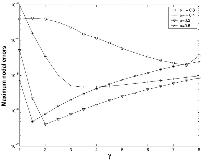
Fig. 1: The left nodal error ${\rm max}_{0\leq n\leq N}\,||U_{h-}^{n}-u(t_{n})||$ as a function of $\gamma$, for $\alpha=-0.8,-0.4,0.2$ and $0.6$, when $M=512$ and $N=64$ (so $h^{2}=k^{3}$).

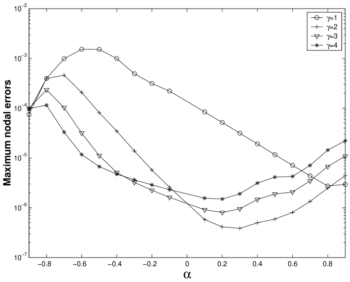
Fig. 2: The left nodal error ${\rm max}_{0\leq n\leq N}\,||U_{h-}^{n}-u(t_{n})||$ as a function of $\alpha$, for $\gamma=1$, 2, 3, 4, when $M=512$ and $N=64$ (so $k^{3}=h^{2}$).

Table 5: The uniform DG error after postprocessing, $\|U^{\sharp}_{h}-u\|_{J,12}$, and its rate of convergence, when $\alpha=-0.3$, for different mesh gradings $\gamma$.

$N$	$\gamma=1$		$\gamma=2$		$\gamma=3$		$\gamma=3.9$
20	3.79e-02		4.52e-03		1.46e-03		8.13e-04
40	2.37e-02	0.675	1.68e-03	1.425	3.27e-04	2.154	1.20e-04	2.763
80	1.44e-02	0.716	6.31e-04	1.416	7.49e-05	2.127	1.79e-05	2.743
160	8.74e-03	0.724	2.38e-04	1.410	1.73e-05	2.113	2.69e-06	2.735

Table 6: The uniform DG error after postprocessing, $\|U^{\sharp}_{h}-u\|_{J,12}$, and its rate of convergence, when $\alpha=+0.3$, for different mesh gradings $\gamma$.

$N$	$\gamma=1$		$\gamma=1.5$		$\gamma=2$		$\gamma=2.35$
20	2.51e-03		4.38e-04		1.56e-04		1.89e-04
40	1.16e-03	1.120	1.22e-04	1.845	2.72e-05	2.515	2.29e-05	3.046
80	5.02e-04	1.205	3.34e-05	1.867	4.59e-06	2.568	2.80e-06	3.029
160	2.12e-04	1.245	8.88e-06	1.911	7.63e-07	2.588	3.44e-07	3.024

7.3 Global error after post-processing

We introduce a finer mesh

$$\mathcal{G}^{N,m}=\{\,t_{j-1}+\ell k_{j}/m:\text{$j=1$, 2, \ldots, $N$ and $\ell=0$, 1, \ldots, $m$}\,\},$$ (58)

and define the discrete maximum norm $\|v\|_{J,m}=\max_{t\in\mathcal{G}^{N,m}}\|v(t)\|$, so that, for sufficiently large values of $m$, $\|U-u\|_{J,m}$ approximates the global error $\|U-u\|_{J}$. Now, in addition to the regularity assumptions (54) and (55), we require that $u$ satisfies (39). In fact, we see from (53) and (56) that, with $\mu=-1$,

$$\bigl{(}t^{j-1}\|\partial_{t}^{j}u(t)\|\bigr{)}^{2}\leq C\bigl{(}t^{(1+\alpha)-1}\bigr{)}^{2}\sum_{n=0}^{\infty}\omega_{n}^{-2}\leq C\bigl{(}t^{(1+\alpha)-1}\bigr{)}^{2},$$

so (39) holds for ${\sigma^{\sharp}}=1+\alpha$. Using Theorem 15 (cf. Subsection 6.4) and (57) with ${\sigma^{\sharp}}=(1+\alpha)<\sigma\approx\tfrac{5}{4}(1+\alpha)$, we expect

$$\|U^{\sharp}_{h}-u\|_{J}\leq Ch^{2}+C\times\begin{cases}k^{\gamma{\sigma^{\sharp}}},&1\leq\gamma\leq(3+\alpha_{-})/{\sigma^{\sharp}},\\ k^{3+\alpha_{-}},&\gamma>(3+\alpha_{-})/{\sigma^{\sharp}}.\end{cases}$$

We observe this convergence behaviour in Tables 6 and 6.

8 Concluding remarks

We have analysed a piecewise-linear DG method for the time discretization of (1) — a fractional diffusion ($-1<\alpha<0$) or wave ($0<\alpha<1$) equation — and proved superconvergence at the nodes, generalizing a known result for the classical heat equation. Numerical experiments indicate that our theoretical error bounds are sharp if $\alpha>0$, but not if $\alpha<0$. For generic regular data $u_{0}$ and $f$, derivatives of the exact solution are singular as $t\to 0$, but nevertheless by employing non-uniform time steps we achieve a high convergence rate of $O(k^{3+\alpha_{-}})$. After postprocessing the solution, the same high accuracy is achieved for all $t$, not just at the nodes. We have also proved that the additional error arising from a spatial discretization by continuous piecewise-linear finite elements is essentially $O(h^{2})$. In future work, we aim to treat the case when the initial data $u_{0}$ is not smooth.

References

- [1] C.-M. Chen, F. Liu, V. Anh, and I. Turner, Numerical schemes with high spatial accuracy for a variable-order anomalous subdiffusion equation, SIAM J. Sci. Comput., 32 (2010), pp. 1740–1760.
- [2] , Numerical methods for solving a two-dimensional variable-order anomalous subdiffusion equation, Math. Comp., 81 (2012), pp. 345–366.
- [3] E. Cuesta, C. Lubich, and C. Palencia, Convolution quadrature time discretization of fractional diffusion-wave equations, Math. Comp., 75 (2006), pp. 673–696.
- [4] E. Cuesta and C. Palencia, A fractional trapezoidal rule for integro-differential equations of fractional order in Banach spaces, Appl. Numer. Math., 45 (2003), pp. 139–159.
- [5] , A numerical method for an integro-differential equation with memory in Banach spaces: qualitative properties, SIAM J. Numer. Anal., 41 (2003), pp. 1232–1241.
- [6] M. Cui, Compact finite difference method for the fractional diffusion equation, J. Comput. Phys., 228 (2009), pp. 7792–7804.
- [7] M. Cui, Compact alternating direction implicit method for two-dimensional time fractional diffusion equation, J. Comput. Phys., 231 (2012), pp. 2621–2633.
- [8] , Convergence analysis of high-order compact alternating direction implicit schemes for the two-dimensional time fractional diffusion equation, Numer. Algor., (Published online: 2012).
- [9] K. Eriksson, C. Johnson, and V. Thomée, Time discretization of parabolic problems by the discontinuous Galerkin method, M2AN Math. Model. Numer. Anal., 19 (1985), pp. 611–643.
- [10] A. Hanyga, Wave propagation in media with singular memory, Math. Comput. Modelling., 34 (2001), pp. 1399–1421.
- [11] B. Jin, R. Lazarov, and Z. Zhou, Error estimates for a semidiscrete finite element method for fractional order parabolic equations. Preprint, arXiv:1204.38884v1.
- [12] A. A. Kilbas, H. M. Srivastava, and J. J. Trujillo, Theory and Applications of Fractional Differential Equations, vol. 204 of North-Holland Mathematics Studies, North–Holland, Amsterdam, 2006.
- [13] T. A. M. Langlands and B. I. Henry, The accuracy and stability of an implicit solution method for the fractional diffusion equation, J. Comput. Phys., 205 (2005), pp. 719–736.
- [14] F. Liu, C. Yang, and K. Burrage, Numerical method and analytical technique of the modified anomalous subdiffusion equation with a nonlinear source term, J. Comput. Appl. Math., 231 (2009), pp. 160–176.
- [15] M. López-Fernández and C. Palencia, On the numerical inversion of the Laplace transform of certain holomorphic functions, Appl. Numer. Math., 51 (2004), pp. 289–303.
- [16] M. López-Fernandez, C. Palencia, and A. Schädle, A spectral order method for inverting sectorial Laplace transforms, SIAM J. Numer. Anal., 44 (2006), pp. 1332–1350.
- [17] F. Mainardi and P. Paradisi, Fractional diffusive waves, J. Comput. Acoustics, 9 (2001), pp. 1417–1436.
- [18] A. M. Mathai, R. K. Saxena, and H. J. Haubold, The H-Function: Theory and Applications, Springer, 2010.
- [19] W. McLean, Regularity of solutions to a time-fractional diffusion equation, ANZIAM J., 52 (2010), pp. 123–138.
- [20] , Fast summation by interval clustering for an evolution equation with memory. Preprint, arXiv:1203.4032v1, 2012.
- [21] W. McLean and K. Mustapha, A second-order accurate numerical method for a fractional wave equation, Numer. Math., 105 (2007), pp. 481–510.
- [22] , Convergence analysis of a discontinuous Galerkin method for a sub-diffusion equation, Numer. Algor., 52 (2009), pp. 69–88.
- [23] W. McLean and V. Thomée, Numerical solution of an evolution equation with a positive-type memory term, ANZIAM J., 35 (1993), pp. 23–70.
- [24] W. McLean and V. Thomée, Numerical solution via Laplace transforms of a fractional order evolution equation, J. Integral Equations Appl., 22 (2010), pp. 57–94.
- [25] W. McLean, V. Thomée, and L. B. Wahlbin, Discretization with variable time steps of an evolution equation with a positive-type memory term, J. Comput. Appl. Math., 69 (1996), pp. 49–69.
- [26] R. Metzler and J. Klafter, The random walk’s guide to anomalous diffusion: a fractional dynamics approach, Physics Reports, 339 (2000), pp. 1–77.
- [27] , The restaurant at the end of the random walk: Recent developments in the description of anomalous transport by fractional dynamics, J. Phys. A, 37 (2004), pp. R161–R208.
- [28] K. Mustapha, An implicit finite difference time-stepping method for a sub-diffusion equation, with spatial discretization by finite elements, IMA Journal Numer. Anal., 31 (2011), pp. 719–739.
- [29] K. Mustapha and J. AlMuttawa, A finite difference method for an anomalous sub-diffusion equation, theory and applications, Numer. Algor., (2012).
- [30] K. Mustapha and W. McLean, Discontinuous Galerkin method for an evolution equation with a memory term of positive type, Math. Comp., 78 (2009), pp. 1975–1995.
- [31] , Piecewise-linear, discontinuous Galerkin method for a fractional diffusion equation, Numer. Algor., 56 (2011), pp. 159–184.
- [32] , Uniform convergence for a discontinuous Galerkin, time stepping method applied to a fractional diffusion equation, IMA J. Numer. Anal., (2012).
- [33] Y. nan Zhang and Z. zhong Sun, Alternating direction implicit schemes for the two-dimensional fractional sub-diffusion equation, J. Comput. Phys., 230 (2011), pp. 8713–8728.
- [34] I. Podlubny, Fractional Differential Equations, vol. 198 of Mathematics in Science and Engineering, Academic Press, San Diego, 1999.
- [35] J. Prüss, Evolutionary Integral Equations and Applications, vol. 87 of Monographs in Mathematics, Birkhäuser, Basel, 1993.
- [36] J. M. Sanz-Serna, A numerical method for a partial integro-differential equation, SIAM J. Numer. Anal., 25 (1988), pp. 319–327.
- [37] A. Schädle, M. López-Fernández, and C. Lubich, Fast and oblivious convolution quadrature, SIAM J. Sci. Comput., 28 (2006), pp. 421–438.
- [38] P. R. Smith, I. E. G. Morrison, K. M. Wilson, N. Fernández, and R. J. Cherry, Anomalous diffusion of major histocompatability complex class I molecules on hela cells determined by single particle tracking, Biophys. J., 76 (1999), pp. 3331–3344.
- [39] I. Sokolov and J. Klafter, From diffusion to anomalous diffusion: A century after Einstein’s Brownian motion, Chaos, 15 (2005), p. 026103.
- [40] V. E. Tarasov, Fractional Dynamics: Applications of Fractional Calculus to Dynamics of Particles, Fields and Media (Nonlinear Physical Science), Springer, 2010.
- [41] H. Wang and K. Wang, An alternating-direction finite difference method for two-dimensional fractional diffusion equations, J. Comput. Phys., 230 (2011), pp. 7830–7839.
- [42] S. B. Yuste, Weighted average finite difference methods for fractional diffusion equations, J. Comput. Phys., 216 (2006), pp. 264–274.
- [43] S. B. Yuste and L. Acedo, An explicit finite difference method and a new von Neumann-type stability analysis for fractional diffusion equations, SIAM J. Numer. Anal., 42 (2005), pp. 1862–1874.
- [44] P. Zhuang, F. Liu, V. Anh, and I. Turner, New solution and analytical techniques of the implicit numerical methods for the anomalous sub-diffusion equation, SIAM J. Numer. Anal., 46 (2008), pp. 1079–1095.
- [45] , Stability and convergence of an implicit numerical method for the nonlinear fractional reaction-subdiffusion process, IMA J. Appl. Math., 74 (2009), pp. 645–667.