Symmetry protected topological (SPT) states are short-range entangled states with symmetry, which have symmetry protected gapless edge states around a gapped bulk. Recently, we proposed a systematic construction of SPT phases in interacting bosonic systems, however it is not very clear what is the form of the low energy excitations on the gapless edge. In this paper, we answer this question for two dimensional bosonic SPT phases with $\mathbb{Z}_{N}$ and $U(1)$ symmetry. We find that while the low energy modes of the gapless edges are non-chiral, symmetry acts on them in a chiral way, i.e. acts on the right movers and the left movers differently. This special realization of symmetry protects the gaplessness of the otherwise unstable edge states by prohibiting a direct scattering between the left and right movers. Moreover, understanding of the low energy effective theory leads to experimental predictions about the SPT phases. In particular, we find that all the 2D $U(1)$ SPT phases have even integer quantized Hall conductance.

Chiral symmetry on the edge of 2D symmetry protected topological phases

Introduction – A recent study shows that gapped quantum states belong to two classes: short-range entangled and long-range entangled.Chen et al. (2010) The long-range entanglement (i.e. the topological orderWen (1990)) in the bulk of states is manifested in the existence of gapless edge modes or degenerate edge sectors. The short-range entangled states are trivial and all belong to the same phase if there is no symmetry. However, with symmetry, even short-range entangled states can belong to different phases. Those phases are called symmetry protected topological (SPT) phases. The symmetric short-range entanglement (i.e. the SPT order) is also manifested in the existence of gapless edge modes around a gapped bulk if the symmetry is not broken. For example, two and three dimensional topological insulatorsKane and Mele (2005a); Bernevig and Zhang (2006); Kane and Mele (2005b); Moore and Balents (2007); Fu et al. (2007); Qi et al. (2008) have a gapped insulating bulk but host gapless fermion modes with special spin configurations Wu et al. (2006); Fu et al. (2007); Moore (2009) on the edge under the protection of time reversal symmetry. The experimental detection of such edge modesKönig et al. (2007); Hsieh et al. (2009); Chen et al. (2009) has attracted much attention and a lot of efforts have been put into the exploration of new SPT phases.

Recently, we presented a systematic construction of SPT phases in bosonic systemsChen et al. (2011), hence extending the understanding of SPT phases from free fermion systems like topological insulators to systems with strong interactions. We showed that there is a one-to-one correspondence between 2D bosonic SPT phases with symmetry $G$ and elements in the third cohomology group ${\cal H}^{3}[G,U(1)]$. Moreover, we proved thatChen et al. (2011) due to the existence of the special effective non-onsite symmetries on the edge of the constructed SPT phases which are related to the nontrivial elements in ${\cal H}^{3}[G,U(1)]$, the edge states must be gapless as long as symmetry is not broken. However, it is not clear what is the form of the gapless edge states, especially the experimentally more relevant low energy part.

A low energy effective edge theory is desired because it could provide a simple understanding of why the gapless edge is stable in these SPT phases. For example, understanding of the low energy ‘helical’ edgeWu et al. (2006) in 2D topological insulators enables us to see that some of the relevant gapping terms are prohibited due to time reversal symmetry. Moreover, low energy excitations are directly related to the response of the SPT phases to various experimental probes, which has led to many proposals about detecting the exotic properties of topological insulatorsFu and Kane (2008, 2007); Qi et al. (2006, 2008); Essin et al. (2009); Tanaka et al. (2009). Such an understanding is hence also important for the experimental realization of bosonic SPT phases.

In this paper, we study the low energy effective edge theory of the 2D bosonic SPT phases with $\mathbb{Z}_{N}$ and $U(1)$ symmetry. We find that the gapless states on the 1D edge is non-chiral, as it should be due of the lack of intrinsic topological orderWen (1995) in the system. The special feature of the edge states lies in the way symmetry is realized. In particular, we find that symmetry is realized chirally at low energy, i.e. in an inequivalent way on the right and left movers. Because of the existence of this chiral symmetry, the direct scattering between the left and right moving branches of the low energy excitations is prohibited which provides protection to the gapless edge.

We would like to mention that people have used $U(1)\times U(1)$ Chern-Simons theoryLevin (2012); Lu and Vishwanath (2012) and $SU(2)$ non-linear $\sigma$-modelLiu and Wen (2012) to construct the edge states of the $U(1)$ SPT phases. However, it is not clear whether we have obtained the edge states for all of the $U(1)$ SPT phases using those field theory approaches. The construction presented in this paper has the advantage of having a direction connection to the third cohomology group ${\cal H}^{3}[U(1),U(1)]$. So we are sure that we have obtained the edge states for all of the $U(1)$ SPT phases.

We would also like to point out that the chiral symmetry leads to a chiral response of the system to externally coupled gauge field even though the edge state as a whole is non-chiral. In particular, we find that all of the $U(1)$ SPT phases have an even-integer quantized Hall conductance.

LABEL:CLW1141,CGLW1172 show that, due to the short range entanglement in SPT phases, the edge of the systems exists as a purely local 1D system with a special non-onsite symmetry related to group cohomology. This enables us to study the edge physics in 1D without worrying about the 2D bulk. We will start with an exact diagonalization of the edge Hamiltonian in the $\mathbb{Z}_{2}$ SPT phase constructed in LABEL:CLW1141. Insights from this model are then generalized to construct a 1D rotor model with different symmetries realizing the edge states of all $\mathbb{Z}_{N}$ and $U(1)$ SPT phases. Some useful formulas of the third group cohomology ${\cal H}^{3}[G,U(1)]$ are reviewed in appendix AI.

Edge state of $\mathbb{Z}_{2}$ SPT phase – In LABEL:CLW1141 we presented an explicit construction of a nontrivial bosonic SPT phase with $\mathbb{Z}_{2}$ symmetry. The edge Hilbert space is identified as a local 1D spin $1/2$ chain. The spin chain satisfies a $\mathbb{Z}_{2}$ symmetry constraint given by

$$U_{2}=\prod_{i}X_{i}\prod_{i}CZ_{i,i+1}$$ (1)

where $X$,$Y$ and $Z$ are the Pauli matrices and $CZ$ acts on two spins as $CZ=|{00}\rangle\langle{00}|+|{01}\rangle\langle{01}|+|{10}\rangle\langle{10}|-|{11}\rangle\langle{11}|$. We showed in LABEL:CLW1141 that this non-onsite symmetry operator is related to the nontrivial element in the third cohomology group of $\mathbb{Z}_{2}$ and hence the edge state must be gapless if symmetry is not broken. Here we study one possible form of the edge Hamiltonian which satisfies this symmetry

$$H_{2}=\sum_{i}X_{i}+Z_{i-1}X_{i}Z_{i+1}$$ (2)

This Hamiltonian is gapless because we can map this model to an $XY$ model. The mapping proceeds as follows: conjugate the Hamiltonian with $CZ$ operators on spin $2i-1$ and $2i$ and then change between $X$ and $Z$ basis on every $(2i-1)$th spin. The Hamiltonian then becomes

$$H_{2}^{\prime}=\sum_{i}X_{i-1}X_{i}+Z_{i-1}Z_{i}$$ (3)

Therefore, the low energy effective theory of this model is that of a compactified boson field $\varphi(x)$ with Lagrangian density

$$\mathcal{L}=\frac{1}{2}\left[(\partial_{t}\varphi)^{2}-v^{2}(\partial_{x}\varphi)^{2}\right]$$ (4)

This is a simple gapless state with both left and right movers and can be easily gapped out with a mass term such as the magnetic field in the $z$ direction $B_{z}(\sum_{i}Z_{i})$. However, such a term is no longer allowed when the transformed $\mathbb{Z}_{2}$ symmetry operation is taken into account:

$$U_{2}^{\prime}=\prod_{2i}CX_{2i,2i-1}\prod_{2i}Z_{2i-1}X_{2i}\prod_{2i}CX_{2i,2i+1}$$ (5)

where $CX_{i,j}$ acts on spin $i$ and $j$ as $CX=|{00}\rangle\langle{00}|+|{01}\rangle\langle{01}|+|{11}\rangle\langle{10}|+|{10}\rangle\langle{11}|$. This symmetry constraint prevents any term from gapping the Hamiltonian without breaking the symmetry.

To see more clearly how this symmetry protects the gaplessness of the system, we study how it acts on the low energies modes. We perform an exact diagonalization of the $XY$ Hamiltonian Eqn.(3) for a system of $16$ spins and identify the free boson modes. Then we calculate the $\mathbb{Z}_{2}$ quantum number on these modes as shown in Fig. 1. Note that $U_{2}^{\prime}$ is not translational invariant and does not commute with the $U(1)$ symmetry of the $XY$ model $\prod_{j}e^{i\theta Y_{j}}$, therefore the free boson modes are not exact eigenstates of the $\mathbb{Z}_{2}$ symmetry. However, at low energy, the $\mathbb{Z}_{2}$ quantum number becomes exact as the system size gets larger and in Fig. 1 we plot the asymptotic $\mathbb{Z}_{2}$ quantum number of the low energy states.

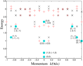
Figure 1: Low energy states of $XY$ model $H_{2}^{\prime}$(Eqn.(3)). $x$-axis is lattice momentum $k/(\pi/a)$, where $a$ is the lattice spacing. $y$-axis is energy with ground state energy set to $0$ and first excited state energy normalized to $1/4$. $+$ represents positive $\mathbb{Z}_{2}$ quantum number and $\times$ represents negative $\mathbb{Z}_{2}$ quantum number. Total boson number $l$ and winding number $m$ are labeled as $(l,m)$ for each primary field, represented by the shaded $+$ or $\times$. States in the same conformal tower have the same $l$ and $m$.

From Fig. 1, we can see that the $\mathbb{Z}_{2}$ quantum number of each state only depends on the quantum number of the zero modes. The zero modes are described by two integers: the total boson number $l$ and the winding number $m$, and the $\mathbb{Z}_{2}$ symmetry at low energy acts as $U_{2}^{\prime}\sim(-)^{l+m}$. From Fig. 1, we also see that the primary fields labeled by $(l,m)$ have the following left- and right-scaling dimensions: $(h_{R},h_{L})=(\frac{(l+2m)^{2}}{8},\frac{(l-2m)^{2}}{8})$.

For the trivial $\mathbb{Z}_{2}$ SPT phase, the onsite $\mathbb{Z}_{2}$ transformation at low energy acts as $U_{2}^{\prime}\sim(-)^{l}$, which is a non-chiral action. For the non-trivial $\mathbb{Z}_{2}$ SPT phase, we see that the non-onsite $\mathbb{Z}_{2}$ transformation at low energy acts as $U_{2}^{\prime}\sim(-)^{l+m}$. We call such an $m$-dependent $U_{2}^{\prime}$ a chiral symmetry operation.

From the chiral symmetry operation, we can have a simple (although not general) understanding of why some of the gap opening perturbations cannot appear in this edge theory. For example, the simplest mass term in the free boson theory $\int dx\cos(\varphi(x))$ contains a direct scattering term $\varphi_{R}(x)\varphi_{L}(x)$ between the left and right movers which carries a nontrivial quantum number under this $\mathbb{Z}_{2}$ symmetry and is hence not allowed. This result is consistent with that obtained by Levin $\&$ GuLevin and Gu (2012).

Edge state of $\mathbb{Z}_{N}$ SPT phase – Understanding of how symmetry acts chirally on the edge state of the $\mathbb{Z}_{2}$ SPT phase suggests that similar situations might appear in other SPT phases as well. In this section we are going to show that it is indeed the case for $\mathbb{Z}_{N}$ bosonic SPT phases. From the group cohomology construction, we know that there are $N$ $\mathbb{Z}_{N}$-SPT phases which form a $\mathbb{Z}_{N}$ group among themselves. We are going to construct 1D rotor models to realize the edge state in each SPT phase which satisfies certain non-onsite symmetry related to the nontrivial elements in ${\cal H}^{3}[\mathbb{Z}_{N},U(1)]$. From these models we can see explicitly how the symmetry acts in a chiral way on the low energy states. Taking the limit of $N\to\infty$ in $\mathbb{Z}_{N}$ will lead to the understanding of the edge states in $U(1)$ SPT phases which we discuss in the next section. Note that the choice of the local Hilbert space on the edge, here a quantum rotor, is arbitrary and will not affect the universal physics of the SPT phase as long as the effective symmetry belongs to the same cohomology class.

Consider a 1D chain of quantum rotors describe by $\{\varphi_{i}\}\in(-\pi,\pi]$ with conjugate momentum $\{L_{i}\}$. The dynamics of the chain is given by Hamiltonian

$$H_{r}=\sum_{i}(L_{i})^{2}+V\cos(\varphi_{i}-\varphi_{i-1})$$ (6)

When $V>>1$, the system is in the gapless superfluid phase. At low energy, $\varphi$ varies smoothly along the chain. The gapless low energy effective theory is again described by a compactified boson field $\varphi(x)$ with compactification radius $1$. The low energy excitations contain both left and right moving bosons.

The generator of the non-onsite $\mathbb{Z}_{N}$ symmetry related to the $M$th element ($M=0,...,N-1$) of the cohomology group, hence the $M$th SPT phase with $\mathbb{Z}_{N}$ symmetry, takes the following form in this rotor chain:

$$U^{(M)}_{N}=\prod_{i}CP^{(M)}_{i,i+1}\prod_{i}e^{i2\pi L_{i}/N}$$ (7)

where $CP^{(M)}_{i,i+1}$ acts on two neighboring rotors and depends on $M$ as

$$CP^{(M)}_{i,i+1}=\int d\varphi_{i}d\varphi_{i+1}e^{iM(\varphi_{i+1}-\varphi_{i})_{r}/N}|{\varphi_{i}\varphi_{i+1}}\rangle\langle{\varphi_{i}\varphi_{i+1}}|$$

Here we need to be careful with the phase factor $e^{iM(\varphi_{i+1}-\varphi_{i})/N}$ because it is not a single-valued function. We confine $\varphi_{i+1}-\varphi_{i}$ to be within $(-\pi,\pi]$ and denote it as $(\varphi_{i+1}-\varphi_{i})_{r}$. Then $e^{iM(\varphi_{i+1}-\varphi_{i})_{r}/N}$ becomes single valued but also discontinuous when $\varphi_{i+1}-\varphi_{i}\sim\pm\pi$. The discontinuity will not be a problem for us in the following discussion. Note that it is important that $e^{iM(\varphi_{i+1}-\varphi_{i})_{r}/N}\neq e^{iM\varphi_{i+1}/N}/e^{iM\varphi_{i}/N}$, because otherwise the symmetry factors into onsite operations and becomes trivial. We show in appendix CIII that $U^{M}_{N}$ indeed generates a $\mathbb{Z}_{N}$ symmetry. Moreover from its matrix product unitary operator representation we find that the transformation among the representing tensors are indeed related to the $M$th element in the cohomology group ${\cal H}^{3}[\mathbb{Z}_{N},U(1)]$. Therefore, the 1D rotor model represents one possible realization of the edge states in the corresponding SPT phases. (The matrix product unitary operator formalism and its relation to group cohomology was studied in LABEL:CLW1141 and we review the main results in appendix BII).

The symmetry operator $U^{(M)}_{N}$ has a complicated form but its physical meaning will become clear if we consider its action on the low energy states of the rotor model in Eqn.(6). First the $\prod_{i}e^{i2\pi L_{i}/N}$ part rotates all rotors by the same angle $2\pi/N$, which can be equivalently written as $e^{i2\pi L/N}$ with $L=\sum_{i}L_{i}$ being the total angular momentum of the rotors. At low energy, $L$ is the total boson number with integer values $l$. Moreover, at low energy $\varphi$ varies smoothly along the chain therefore $(\varphi_{i+1}-\varphi_{i})_{r}\sim\partial_{x}\varphi(x)dx$ and $CP^{(M)}_{i,i+1}$ adds a phase factor to the differential change in $\varphi$ along the chain. Multiplied along the whole chain $\prod_{i}CP^{(M)}_{i,i+1}$ is equal to $e^{i2\pi M(\int dx\partial_{x}\varphi(x))/N}=e^{i2\pi Mm/N}$ where $m$ is the winding number of the boson field $\varphi(x)$ along the chain. Put together we find that the symmetry acts on the low energy modes as

$$U^{(M)}_{N}\sim e^{i2\pi(l+Mm)/N}$$ (8)

If $M$ is zero, this symmetry comes from a trivial SPT phase and $U^{(0)}_{N}$ depends only on $l$ which involves the left and right movers equally,as one can see from right- and left-scaling dimensions $(h_{R},h_{L})=(\frac{(l+2m)^{2}}{8},\frac{(l-2m)^{2}}{8})$. However, when $M$ is nonzero, this symmetry comes from a nontrivial SPT phase and $U^{(M)}_{N}$ depends on $l+Mm$ which involves the left and right mover in an unequal way. Put it differently, the symmetry on the edge of nontrivial $\mathbb{Z}_{N}$ SPT phases acts chirally. In particular, when $M=2$, the symmetry will act only on the right movers. Similar to the discussion in the $\mathbb{Z}_{2}$ case, we can see that the chiral symmetry protects the gaplessness of the edge by preventing direct scattering between the left and right branches.

One may notice that $H_{r}$(Eqn.(6)) does not exactly commute with the symmetry $U^{(M)}_{N}$, but this will not be a problem for our discussions. We note that the potential term $\cos(\varphi_{i}-\varphi_{i-1})$ does commute with $U^{(M)}_{N}$. The kinetic term $(L_{i})^{2}$ commute with the part that rotates $\varphi$ but not the phase factor $e^{iM(\varphi_{i+1}-\varphi_{i})_{r}/N}$. However, at low energy, $(\varphi_{i+1}-\varphi_{i})\to 0$, therefore this term becomes irrelevant locally and commutation between the Hamiltonian and the symmetry operator is restored. At high energy, in order for the Hamiltonian to satisfy the symmetry, we can change the kinetic term to $\sum^{N-1}_{k=0}\left(U^{(M)}_{N}\right)^{k}(L_{i})^{2}\left(U^{(M)}_{N}\right)^{-k}$. The high energy dynamics will be changed. However, because $V>>1$ and we know that the modified Hamiltonian does not break the $U(1)$ symmetry of the rotor model and the system cannot be gapped (due to the nontrivial cohomology class related to the symmetry), the system remains in the superfluid phase. The change in the kinetic term does not affect our discussion about low energy effective physics.

Edge state of $U(1)$ SPT phase – Taking the limit of $N\to\infty$, we can generalize our understanding of $\mathbb{Z}_{N}$ SPT phases to $U(1)$ SPT phases. As we show in this section, the chiral symmetry action on the low energy effective modes on the edge of the $U(1)$ SPT phases leads to a chiral response of the system to externally coupled $U(1)$ gauge field, even though the low energy edge state is non-chiral. We calculate explicitly the quantized Hall conductance in these SPT phases from the commutator of local density operators on the edge and find that they are quantized to even integer multiples of $\sigma_{H}=e^{2}/h$. In these SPT phases, a nonzero $U(1)$ Hall conductance exists despite a zero thermal Hall conductance.

¿From group cohomology, we know that there are infinite 2D bosonic SPT phases with $U(1)$ symmetry which form the integer group $\mathbb{Z}$ among themselves. Generalizing the discussion in the previous section we find that the low energy effective theory can be a $c=1$ free boson theory and the $U(1)$ symmetry acts on the low energy modes as $e^{i\alpha(l+Mm)}$, where $\alpha\in[0,2\pi)$, $l$ is the total boson number, $m$ is the winding number and $M\in\mathbb{Z}$ labels the $U(1)$ SPT phase. The local density operator of this $U(1)$ charge is given by

$$\rho(x)=\Pi(x)+\frac{M}{2\pi}\partial_{x}\varphi(x),$$ (9)

with $\Pi(x)$ being the conjugate momentum of the boson field $\varphi(x)$, because the spatial integration of this density operator gives rise to the generator of the $U(1)$ symmetry $\int dx\rho(x)=l+Mm$. The commutator between local density operators is given by

$$[\rho(x),\rho(x^{\prime})]=-i\frac{2M}{2\pi}\delta^{\prime}(x-x^{\prime}).$$ (10)

This term will give rise to a quantized Hall conductance along the edge when the system is coupled to an external $U(1)$ gauge field. Compared to the commutator between local density operators of a single chiral fermion

$$[\rho_{cf}(x),\rho_{cf}(x^{\prime})]=-i\frac{1}{2\pi}\delta^{\prime}(x-x^{\prime}),$$ (11)

we see that the Hall conductance is quantized to even integer $2M$ multiples of $\sigma_{H}=e^{2}/h$.

As a consistency check we see that the quantized Hall conductance is a universal feature of the edge states in the bosonic $U(1)$ SPT phases and does not depend on the particular form the $U(1)$ symmetry is realized on the edge. Indeed, the $U(1)$ symmetry can be realized as $e^{i\alpha(Kl+K^{\prime}m)}$, with arbitrary $K,K^{\prime}\in\mathbb{Z}$. From the group cohomology calculation (reviewed in appendix BII) we find that it belongs to the cohomology class labeled by $M=KK^{\prime}$. From the calculation of the commutator between local density operators, we see that the magnitude of the commutator is proportional also to $M=KK^{\prime}$. Therefore, the Hall conductance depends only on the cohomology class–hence the SPT phase–the system is in and not on the details of the dynamics in the system.

Discussion – In this paper, we have construct the gapless edge states for each of the bosonic $\mathbb{Z}_{N}$ or $U(1)$ SPT phases in 2D. We show that those edge states are described by a $c=1$ non-chiral free boson theory where the symmetry acts chirally on the low energy modes. The chiral realization of the symmetry not only prevents some simple mass terms from gapping out the system but also leads to a chiral response of the system to external gauge fields. We demonstrate this by constructing explicit 1D lattice models constrained by a non-onsite symmetry related to each nontrivial cohomology classes. Our result indicates that the field theory approach based on the $U(1)\times U(1)$ Chern-Simons theoryLevin (2012); Lu and Vishwanath (2012) and $SU(2)$ non-linear $\sigma$-modelLiu and Wen (2012) indeed produce all of the $U(1)$ SPT phases.

We want to emphasize that although we have focused exclusively on the 1D edge, a 2D bulk having the 1D chain as its edge always exists and can be constructed by treating a 1D ring as a single site and then putting the sites together. Note that while the stability and chiral response of the edge in SPT phases are very similar to that of the edge in quantum Hall systems, the underlying reason is very different. The quantum Hall edge states are chiral in its own, which remains gapless without the protection of any symmetry and leads to a nonzero thermal Hall conductance.

Finally, we want to point out that the edge theory constructed in this paper is only one possible form of realization. It is possible that other gapless theories can be realized on the edge of SPT phases, for example with central charge not equal to $1$. It would be interesting to understand in general what kind of gapless theories are possible and what their universal features are.

We would like to thank Zheng-Cheng Gu and Senthil Todadri for discussions. This work is supported by NSF DMR-1005541 and NSFC 11074140.

I Appendix A: The third group cohomology ${\cal H}^{3}[G,U(1)]$ for symmetry $G$

In this section, we will briefly describe the group cohomology theory. As we are focusing on 2D SPT phases, we will be interested in the third cohomology group.

For a group $G$, let $M$ be a G-module, which is an abelian group (with multiplication operation) on which $G$ acts compatibly with the multiplication operation (ie the abelian group structure) on $M$:

$$g\cdot(ab)=(g\cdot a)(g\cdot b),\ \ \ \ g\in G,\ \ \ \ a,b\in M.$$ (12)

For the cases studied in this paper, $M$ is simply the $U(1)$ group and $a$ an $U(1)$ phase. The multiplication operation $ab$ is the usual multiplication of the $U(1)$ phases. The group action is trivial: $g\cdot a=a$, $g\in G$, $a=\in U(1)$.

Let $\omega_{n}(g_{1},...,g_{n})$ be a function of $n$ group elements whose value is in the G-module $M$. In other words, $\omega_{n}:G^{n}\to M$. Let ${\cal C}^{n}[G,M]=\{\omega_{n}\}$ be the space of all such functions. Note that ${\cal C}^{n}[G,M]$ is an Abelian group under the function multiplication $\omega^{\prime\prime}_{n}(g_{1},...,g_{n})=\omega_{n}(g_{1},...,g_{n})\omega^{\prime}_{n}(g_{1},...,g_{n})$. We define a map $d_{n}$ from ${\cal C}^{n}[G,U(1)]$ to ${\cal C}^{n+1}[G,U(1)]$:

$$\ \ \ \ (d_{n}\omega_{n})(g_{1},...,g_{n+1})=$$

$$g_{1}\cdot\omega_{n}(g_{2},...,g_{n+1})\omega_{n}^{(-1)^{n+1}}(g_{1},...,g_{n})\times$$

$$\ \ \ \ \ \prod_{i=1}^{n}\omega_{n}^{(-1)^{i}}(g_{1},...,g_{i-1},g_{i}g_{i+1},g_{i+2},...g_{n+1})$$ (13)

Let

$${\cal B}^{n}[G,M]=\{\omega_{n}|\omega_{n}=d_{n-1}\omega_{n-1}|\omega_{n-1}\in{\cal C}^{n-1}[G,M]\}$$ (14)

and

$${\cal Z}^{n}[G,M]=\{\omega_{n}|d_{n}\omega_{n}=1,\omega_{n}\in{\cal C}^{n}[G,M]\}$$ (15)

${\cal B}^{n}[G,M]$ and ${\cal Z}^{n}[G,M]$ are also Abelian groups which satisfy ${\cal B}^{n}[G,M]\subset{\cal Z}^{n}[G,M]$ where ${\cal B}^{1}[G,M]\equiv\{1\}$. ${\cal Z}^{n}[G,M]$ is the group of $n$-cocycles and ${\cal B}^{n}[G,M]$ is the group of $n$-coboundaries. The $n$th cohomology group of $G$ is defined as

$${\cal H}^{n}[G,M]={\cal Z}^{n}[G,M]/{\cal B}^{n}[G,M]$$ (16)

In particular, when $n=3$, from

$$\ \ \ \ (d_{3}\omega_{3})(g_{1},g_{2},g_{3},g_{4})$$

$$=\frac{\omega_{3}(g_{2},g_{3},g_{4})\omega_{3}(g_{1},g_{2}g_{3},g_{4})\omega_{3}(g_{1},g_{2},g_{3})}{\omega_{3}(g_{1}g_{2},g_{3},g_{4})\omega_{3}(g_{1},g_{2},g_{3}g_{4})}$$ (17)

we see that

$${\cal Z}^{3}[G,U(1)]=\{\omega_{3}|$$ (18)

$$\ \ \ \frac{\omega_{3}(g_{2},g_{3},g_{4})\omega_{3}(g_{1},g_{2}g_{3},g_{4})\omega_{3}(g_{1},g_{2},g_{3})}{\omega_{3}(g_{1}g_{2},g_{3},g_{4})\omega_{3}(g_{1},g_{2},g_{3}g_{4})}=1\}.$$

and

$${\cal B}^{3}[G,U(1)]=\{\omega_{3}|\omega_{3}(g_{1},g_{2},g_{3})=\frac{\omega_{2}(g_{2},g_{3})\omega_{2}(g_{1},g_{2}g_{3})}{\omega_{2}(g_{1}g_{2},g_{3})\omega_{2}(g_{1},g_{2})}\},$$ (19)

which give us the third cohomology group ${\cal H}^{3}[G,U(1)]={\cal Z}^{3}[G,U(1)]/{\cal B}^{3}[G,U(1)]$.

II Appendix B: Matrix Product Operator Representation of Symmetry

In LABEL:CLW1141 the symmetry operators on the edge of bosonic SPT phases were represented in the matrix product operator formalism from which their connection to group cohomology is revealed and the non-existence of gapped symmetric states was proved. In this section, we review the matrix product representation of the unitary symmetry operators and how the corresponding cocycle can be calculated from the tensors in the representation.

A matrix product operator acting on a 1D system is given by,Pirvu et al. (2010)

$$O=\sum_{\{i_{k}\},\{i_{k}^{\prime}\}}Tr(T^{i_{1},i^{\prime}_{1}}T^{i_{2},i^{\prime}_{2}}...T^{i_{N},i^{\prime}_{N}})|i^{\prime}_{1}i^{\prime}_{2}...i^{\prime}_{N}\rangle\langle i_{1}i_{2}...i_{N}|$$ (20)

where for fixed $i$ and $i^{\prime}$, $T^{i,i^{\prime}}$ is a matrix with index $\alpha$ and $\beta$. Here we are interested in symmetry transformations, therefore we restrict $O$ to be a unitary operator $U$. Using matrix product representation, $U$ does not have to be an onsite symmetry. $U$ is represented by a rank-four tensor $T^{i,i^{\prime}}_{\alpha,\beta}$ on each site, where $i$ and $i^{\prime}$ are input and output physical indices and $\alpha$, $\beta$ are inner indices.

If $U(g)$’s form a representation of group $G$, then they satisfy $U(g_{1})U(g_{2})=U(g_{1}g_{2})$. Correspondingly, the tensors $T(g_{1})$ and $T(g_{2})$ should have a combined action equivalent to $T(g_{1}g_{2})$. However, the tensor $T(g_{1},g_{2})$ obtained by contracting the output physical index of $T(g_{2})$ with the input physical index of $T(g_{1})$, see Fig. 2, is usually more redundant than $T(g_{1}g_{2})$ and can only be reduced to $T(g_{1}g_{2})$ if certain projection $P_{g_{1},g_{2}}$ is applied to the inner indices (see Fig. 2).

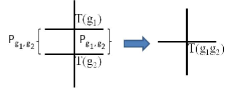
Figure 2: Reduce combination of $T(g_{2})$ and $T(g_{1})$ into $T(g_{1}g_{2})$.

$P_{g_{1},g_{2}}$ is only defined up to an arbitrary phase factor $e^{i\mu(g_{1},g_{2})}$. If the projection operator on the right side $P_{g_{1},g_{2}}$ is changed by the phase factor $e^{i\mu(g_{1},g_{2})}$, the projection operator $P^{\dagger}_{g_{1},g_{2}}$ on the left side is changed by phase factor $e^{-i\mu(g_{1},g_{2})}$. Therefore the total action of $P_{g_{1},g_{2}}$ and $P^{\dagger}_{g_{1},g_{2}}$ on $T(g_{1},g_{2})$ does not change and the reduction procedure illustrated in Fig.2 still works. In the following discussion, we will assume that a particular choice of phase factors have been made for each $P_{g_{1},g_{2}}$.

Nontrivial phase factors appear when we consider the combination of three symmetry tensors $T(g_{1})$, $T(g_{2})$ and $T(g_{3})$. See Fig. 3.

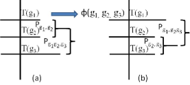
Figure 3: Different ways to reduce combination of $T(g_{3})$, $T(g_{2})$ and $T(g_{1})$ into $T(g_{1}g_{2}g_{3})$. Only the right projection operators are shown. Their combined actions differ by a phase factor $\phi(g_{1},g_{2},g_{3})$.

There are two different ways to reduce the tensors. We can either first reduce the combination of $T(g_{1})$, $T(g_{2})$ and then combine $T(g_{3})$ or first reduce the combination of $T(g_{2})$,$T(g_{3})$ and then combine $T(g_{1})$. The two different ways should be equivalent. More specifically, they should be the same up to phase on the unique block of $T(g_{1},g_{2},g_{3})$ which contributes to matrix contraction along the chain. Denote the projection onto the unique block of $T(g_{1},g_{2},g_{3})$ as $Q_{g_{1},g_{2},g_{3}}$. We find that

$$\begin{array}[]{l}Q_{g_{1},g_{2},g_{3}}(I_{3}\otimes P_{g_{1},g_{2}})P_{g_{1}g_{2},g_{3}}=\\ \phi(g_{1},g_{2},g_{3})Q_{g_{1},g_{2},g_{3}}(P_{g_{2},g_{3}}\otimes I_{1})P_{g_{1},g_{2}g_{3}}\end{array}$$ (21)

¿From this we see that the reduction procedure is associative up to a phase factor $\phi(g_{1},g_{2},g_{3})$. If we then consider the combination of four symmetry tensors in different orders, we can see that $\phi(g_{1},g_{2},g_{3})$ forms a 3-cocycle of group $G$. That is, $\phi(g_{1},g_{2},g_{3})$ satisfies

$$\frac{\phi(g_{2},g_{3},g_{4})\phi(g_{1},g_{2}g_{3},g_{4})\phi(g_{1},g_{2},g_{3})}{\phi(g_{1}g_{2},g_{3},g_{4})\phi(g_{1},g_{2},g_{3}g_{4})}=1$$ (22)

The arbitrary phase factor of $P_{g_{1},g_{2}}$ contributes a coboundary term to $\phi(g_{1},g_{2},g_{3})$. That is, if we change the phase factor of $P_{g_{1},g_{2}}$ by $\mu(g_{1},g_{2})$, then $\phi(g_{1},g_{2},g_{3})$ is changed to

$$\tilde{\phi}(g_{1},g_{2},g_{3})=\phi(g_{1},g_{2},g_{3})\frac{\mu(g_{2},g_{3})\mu(g_{1},g_{2}g_{3})}{\mu(g_{1},g_{2})\mu(g_{1}g_{2},g_{3})}$$ (23)

$\tilde{\phi}(g_{1},g_{2},g_{3})$ still satisfies the cocycle condition and belongs to the same cohomology class as $\phi(g_{1},g_{2},g_{3})$.

III Appendix C: Cohomology class of symmetry operator $U^{(M)}_{N}$ in Eqn.(7)

In this section, we discuss the property of the symmetry operator $U^{(M)}_{N}$ given in Eqn.(7). First we show that $U^{(M)}_{N}$ indeed generates a $\mathbb{Z}_{N}$ symmetry. Next from its matrix product unitary operator representation we find that the transformation among the tensors are indeed related to the $M$th element in the cohomology group ${\cal H}^{3}[\mathbb{Z}_{N},U(1)]$. The calculation of cohomology class goes as described in the previous section. We repeat the definition of $U^{(M)}_{N}$ here

$$U^{(M)}_{N}=\prod_{i}CP^{(M)}_{i,i+1}\prod_{i}e^{i2\pi L_{i}/N}$$ (24)

where $CP^{(M)}_{i,i+1}$ acts on two neighboring rotors and depends on $M$ as

$$CP^{(M)}_{i,i+1}=\int d\varphi_{i}d\varphi_{i+1}e^{iM(\varphi_{i+1}-\varphi_{i})_{r}/N}|{\varphi_{i}\varphi_{i+1}}\rangle\langle{\varphi_{i}\varphi_{i+1}}|$$

Note that $(\varphi_{i+1}-\varphi_{i})_{r}$ represents $\varphi_{i+1}-\varphi_{i}$ to be confined within $(-\pi,\pi]$.

As $\prod_{i}e^{i2\pi L_{i}/N}$ rotates all the $\varphi_{i}$’s by the same angle and $\prod_{i}CP^{(M)}_{i,i+1}$ only depends on the difference between neighboring $\varphi$’s, the two parts in the symmetry operator commutes. Therefore

$$\left(U^{(M)}_{N}\right)^{N}=\prod_{i}\left(CP^{(M)}_{i,i+1}\right)^{N}\prod_{i}\left(e^{i2\pi L_{i}/N}\right)^{N}$$ (25)

As $\prod_{i}\left(CP^{(M)}_{i,i+1}\right)^{N}=I$ and $\prod_{i}\left(e^{i2\pi L_{i}/N}\right)^{N}=e^{i2\pi L}=I$, $U^{(M)}_{N}$ indeed generators a $\mathbb{Z}_{N}$ symmetry on the 1D rotor system.

The matrix product representation of $U^{(M)}_{N}$ is given by

$$\begin{array}[]{l}(T^{\varphi_{0},\varphi_{1}})^{(M)}_{N}(1)=\delta(\varphi_{1}-(\varphi_{0}+\frac{2\pi}{N}))\times\\ \int d\varphi_{\alpha}d\varphi_{\beta}|{\varphi_{\beta}}\rangle\langle{\varphi_{\alpha}}|\delta(\varphi_{\beta}-\varphi_{0})e^{iM(\varphi_{\alpha}-\varphi_{0})_{r}/N}\end{array}$$ (26)

And the tensors representing $\left(U^{(M)}_{N}\right)^{k}$, $k\in\mathbb{Z}_{N}$ are given by

$$\begin{array}[]{l}(T^{\varphi_{0},\varphi_{1}})^{(M)}_{N}(k)=\delta(\varphi_{1}-(\varphi_{0}+\frac{2k\pi}{N}))\times\\ \int d\varphi_{\alpha}d\varphi_{\beta}|{\varphi_{\beta}}\rangle\langle{\varphi_{\alpha}}|\delta(\varphi_{\beta}-\varphi_{0})e^{ikM(\varphi_{\alpha}-\varphi_{0})_{r}/N}\end{array}$$ (27)

Following the calculation described in the previous section, we find that the projection operation when combining $T^{(M)}_{N}(m_{1})$ and $T^{(M)}_{N}(m_{2})$ into $T^{(M)}_{N}((m_{1}+m_{2})_{N})$ is

$$\begin{array}[]{r}P^{(M)}_{N}(m_{1},m_{2})=\int d\varphi_{0}|{m_{2}\frac{2\pi}{N}+\varphi_{0}}\rangle|{\varphi_{0}}\rangle\langle{\varphi_{0}}|\times\\ e^{-iM\varphi_{0}(m_{1}+m_{2}-(m_{1}+m_{2})_{N})/N}\end{array}$$ (28)

where $(m_{1}+m_{2})_{N}$ means addition modulo $N$. When combining $T^{(M)}_{N}(m_{1})$, $T^{(M)}_{N}(m_{2})$ and $T^{(M)}_{N}(m_{3})$, the phase angle in combining $m_{1}$ with $m_{2}$ first and then combining $(m_{1}+m_{2})_{N}$ with $m_{3}$ is

$$\begin{array}[]{ll}&M\varphi_{0}(-m_{1}-m_{2}+(m_{1}+m_{2})_{N}-(m_{1}+m_{2})_{N}-\\ &m_{3}+((m_{1}+m_{2})_{N}+m_{3})_{N})/N\\ =&M\varphi_{0}(-(m_{1}+m_{2}+m_{3})+(m_{1}+m_{2}+m_{3})_{N})/N\end{array}$$ (29)

the phase angle in combining $m_{2}$ with $m_{3}$ first and then combining $m_{1}$ with $(m_{2}+m_{3})_{N}$ is

$$\begin{array}[]{ll}&M\varphi_{0}(-m_{2}-m_{3}+(m_{2}+m_{3})_{N}-m_{1}-\\ &(m_{2}+m_{3})_{N}+(m_{1}+(m_{1}+m_{2})_{N})_{N})/N+\\ &Mm_{1}\frac{2\pi}{N}(-m_{2}-m_{3}+(m_{2}+m_{3})_{N})/N\\ =&M\varphi_{0}(-(m_{1}+m_{2}+m_{3})+(m_{1}+m_{2}+m_{3})_{N})/N+\\ &Mm_{1}\frac{2\pi}{N}(-m_{2}-m_{3}+(m_{2}+m_{3})_{N})/N\end{array}$$ (30)

Therefore, the phase difference is

$$\begin{array}[]{l}\phi^{(M)}_{N}(m_{1},m_{2},m_{3})=\\ e^{iMm_{1}\frac{2\pi}{N}(-m_{2}-m_{3}+(m_{2}+m_{3})_{N})/N}\end{array}$$ (31)

We can check explicitly that $\phi^{(M)}_{N}(m_{1},m_{2},m_{3})$ satisfies the cocycle condition

$$\begin{array}[]{l}\frac{\phi^{(M)}_{N}(m_{2},m_{3},m_{4})\phi^{(M)}_{N}(m_{1},(m_{2}+m_{3})_{N},m_{4})\phi^{(M)}_{N}(m_{1},m_{2},m_{3})}{\phi^{(M)}_{N}((m_{1}+m_{2})_{N},m_{3},m_{4})\phi^{(M)}_{N}(m_{1},m_{2},(m_{3}+m_{4})_{N})}\\ =1\end{array}$$ (32)

Also we see that $\{\phi^{(M)}_{N}\}$, $M=0,...,N-1$, form a $\mathbb{Z}_{N}$ group generated by $\phi^{(1)}_{N}$. Therefore, the tensor $T^{(M)}_{N}$ corresponds to the $M$th element in the cohomology group ${\cal H}^{3}[\mathbb{Z}_{N},U(1)]$.

Similar calculation holds for the $U(1)$ symmetry generated by $e^{i\alpha(Kl+K^{\prime}m)}$, $K,K^{\prime}\in\mathbb{Z}$. The cohomology class is labeled by $M=KK^{\prime}$.

IV Appendix D: Interpretation in terms of fermionization

The free boson theory given in Eqn.(4) can be fermionized and the low energy effective action of the symmetry discussed here can be reinterpreted in terms of a free Dirac fermion. In particular, the fermionized theory has Lagrangian density

$$\mathcal{L}_{f}=\sum_{i=1,2}\psi^{L}_{i}(\partial_{t}+\partial_{x})\psi^{L}_{i}+\psi^{R}_{i}(\partial_{t}-\partial_{x})\psi^{R}_{i}$$ (33)

where $\psi_{1}$ and $\psi_{2}$ are two real fermions, out of which a complex fermion can be defined $\Psi=\psi_{1}+i\psi_{2}$. Note that in order to have a state to state correspondence between the boson and fermion theory, the fermion theory contains both the periodic and anti-periodic sectors.

Since the $\mathbb{Z}_{2}$ symmetry in the nontrivial $\mathbb{Z}_{2}$ SPT phase only act on, say, the right moving sector, one may naively guess that only $\psi_{1}^{R}$ change sign, while $\psi_{2}^{R}$, $\psi_{1}^{L}$, and $\psi_{2}^{L}$ do not change under the $\mathbb{Z}_{2}$ transformation: $(\psi_{1}^{R},\psi_{2}^{R},\psi_{1}^{L},\psi_{2}^{L})\to(-\psi_{1}^{R},\psi_{2}^{R},\psi_{1}^{L},\psi_{2}^{L})$. In this case, the fermion mass term, such as $(\psi_{2}^{R})^{\dagger}\psi_{2}^{L}$, will be allowed by the $\mathbb{Z}_{2}$ symmetry. Such a mass term will reduce the $c=1$ edge state to a $c=\frac{1}{2}$ edge state without breaking the $\mathbb{Z}_{2}$ symmetry. In the following, we will show that the $\mathbb{Z}_{2}$ symmetry is actually realized in a different way. The $c=1$ edge state is stable if the $\mathbb{Z}_{2}$ symmetry is not broken. So the $c=1$ edge state represents the minimal edge state for the $\mathbb{Z}_{2}$ (as well as the $\mathbb{Z}_{N}$ and $U(1)$) SPT phases.

The situation is best illustrated with explicit Jordan-Wigner transformation of the $XY$ model in Eqn.(3). Consider a system of size $N=4n$, $n\in\mathbb{Z}_{+}$. After the Jordan Wigner transformation

$$\Psi_{i}=e^{i\pi\sum^{i-1}_{j=1}Z_{j}}(X_{i}+iY_{i})$$ (34)

$$\Psi^{\dagger}_{i}=e^{i\pi\sum^{i-1}_{j=1}Z_{j}}(X_{i}-iY_{i})$$

The Hamiltonian becomes

$$\begin{array}[]{l}H=H_{a}+H_{b}\\ H_{a}=\sum^{N}_{i=1}(\Psi^{\dagger}_{i+1}\Psi_{i}+\Psi_{i}^{\dagger}\Psi_{i+1})\\ H_{b}=-(P+1)(\Psi^{\dagger}_{1}\Psi_{N}+\Psi_{N}^{\dagger}\Psi_{1})\end{array}$$ (35)

where $P=e^{i\pi\sum_{i=1}^{N}\Psi_{j}^{\dagger}\Psi_{j}}$ is the total fermion parity in the chain and $H_{b}$ is the boundary term which depends on $P$. Therefore, the fermion theory contains two sectors, one with an even number of fermions and therefore anti-periodic boundary condition and one with an odd number of fermions and periodic boundary condition. Without terms mixing the two sectors, we can solve the free fermion Hamiltonian in each sector separately. After Fourier transform, the Hamiltonian becomes

$$H=\sum_{k}\cos\left(\frac{2\pi k}{N}\right)\Psi_{k}^{\dagger}\Psi_{k}$$ (36)

where $k$ takes value $0$, $1$, …, $N-1$ in the periodic sector and $\frac{1}{2}$, $\frac{3}{2}$, … $\frac{2N-1}{2}$ in the anti-periodic sector. The ground state in each sector has all the modes with energy $\leq 0$ filled. Note that with this filling the parity constraint in each sector is automatically satisfied. The ground state energy in the periodic sector is higher than in the anti-periodic sector and the difference is inverse proportional to system size $N$.

Now let’s consider the effect of various perturbations on the system.

The $(l,m)=(1,0)$ operator or the $(-1,0)$ operator in the boson theory (as shown in Fig. 1) corresponds to changing the boundary condition of the Dirac fermion from periodic to anti-periodic. Such operators would totally gap out the edge states. However, from Eqn. (7) and Eqn. (8), we see that both operators carry nontrivial quantum number in all $\mathbb{Z}_{N}$ (and $U(1)$) SPT phases, therefore it is forbidden by the symmetry.

The $(l,m)=(2,0)$ operator in the boson theory corresponds to the pair creation operator $\Psi^{\dagger}_{L}\Psi^{\dagger}_{R}$ in the fermion theory. Its combination with the $(-2,0)$ operator ($\Psi_{R}\Psi_{L}$ in the fermion theory) would gap out the system, but due to the existence of the two sectors the ground state would be two fold degenerate. To see this more explicitly, consider the $XY$ model again where the combination of $(l,m)=(2,0)$ and $(-2,0)$ operators can be realized with an anisotropy term

$$H^{XY}_{(2,0)}=\gamma\sum_{i}X_{i-1}X_{i}-Z_{i-1}Z_{i}$$ (37)

Under Jordan Wigner transformation, it is mapped to the p-wave pairing term

$$\begin{array}[]{l}H_{(2,0)}=H_{a,(2,0)}+H_{b,(2,0)}\\ H_{a,(2,0)}=\gamma\sum^{N}_{i=1}(\Psi^{\dagger}_{i+1}\Psi^{\dagger}_{i}+\Psi_{i}\Psi_{i+1})\\ H_{b,(2,0)}=-\gamma(P+1)(\Psi^{\dagger}_{1}\Psi_{N}+\Psi_{N}^{\dagger}\Psi_{1})\end{array}$$ (38)

Again, we have period boundary condition for $P=-1$ and anti-periodic boundary condition for $P=1$. After Fourier transform, the Hamiltonian at each pair of $k$ and $N-k$ is

$$\begin{array}[]{lll}H_{k,N-k}&=&\cos\left(\frac{2\pi k}{N}\right)(\Psi_{k}^{\dagger}\Psi_{k}+\Psi_{N-k}^{\dagger}\Psi_{N-k})+\\ &&i\gamma\sin\left(\frac{2\pi k}{N}\right)(-\Psi_{k}^{\dagger}\Psi^{\dagger}_{N-k}+\Psi_{N-k}\Psi_{k})\end{array}$$ (39)

The Bogoliubov modes changes smoothly with $\gamma$ and the ground state parity remains invariant. The ground state energy is $\frac{1}{2}\sum_{k}\left(1-(1-\gamma^{2})\sin^{2}\left(\frac{2\pi k}{N}\right)\right)^{1/2}$ and explicit calculation shows that the energy difference of the two sectors (with $k=$ int. and $k=$ int. $+\frac{1}{2}$) becomes exponentially small with nonzero $\gamma$. Therefore, upon adding the $(l,m)=(2,0)$ and $(-2,0)$ terms, the ground state becomes two fold degenerate. Such an operator does carry trivial quantum number in the nontrivial $\mathbb{Z}_{2}$ SPT phase and renders the gapless edge unstable. However, a two fold degeneracy would always be left over in the ground states, indicating a spontaneous $\mathbb{Z}_{2}$ symmetry breaking at the edge.

The $(0,1)$ operator in the boson theory corresponds to a scattering term between the left and right moving fermions $\Psi^{\dagger}_{L}\Psi_{R}$. Its combination with the $(0,-1)$ operator ($\Psi^{\dagger}_{R}\Psi_{L}$ in the fermion theory) would gap out the system. Unlike the $(2,0)$ operator, there is no degeneracy left in the ground state. In the $XY$ model, this corresponds to a staggered coupling constant

$$H^{XY}_{(0,1)}=\gamma\sum_{i}(-1)^{i}\left(X_{i-1}X_{i}+Z_{i-1}Z_{i}\right)$$ (40)

Mapped to fermions, the Hamiltonian at $k$ and $k+\frac{N}{2}$ becomes

$$\begin{array}[]{lll}H_{k,k+\frac{N}{2}}&=&\cos\left(\frac{2\pi k}{N}\right)(\Psi_{k}^{\dagger}\Psi_{k}-\Psi_{k+\frac{N}{2}}^{\dagger}\Psi_{k+\frac{N}{2}})+\\ &&i\gamma\sin\left(\frac{2\pi k}{N}\right)(-\Psi_{k}^{\dagger}\Psi_{k+\frac{N}{2}}+\Psi^{\dagger}_{k+\frac{N}{2}}\Psi_{k})\end{array}$$ (41)

For each pair of $k$ and ${k+\frac{N}{2}}$, there is one positive energy mode and one negative energy mode and we want to fill the negative energy mode with a fermion to obtain to ground state. For the anti-periodic sector, such a construction works since there is a $N/2$ = even number of negative energy modes, and the anti-periodic sector contains an even number of fermions. However, for the periodic sector, such a construction fails since there is a $N/2$ = even number of negative energy modes, and the periodic sector must contain an odd number of fermions. So we have to add an fermion to a positive energy mode (or have a hole in a negative energy mode), to have an odd number of fermions. Therefore, the ground state in the periodic sector has a finite energy gap above the anti-periodic one and the ground state of the whole system is nondegenerate. However, because this term carries nontrivial quantum number in any nontrivial $\mathbb{Z}_{N}$ (and $U(1)$) SPT phases, it is forbidden by the symmetry. For the trivial $\mathbb{Z}_{2}$ SPT phase, the $(0,\pm 1)$ operators are $\mathbb{Z}_{2}$ symmetric operators, and can be added to the edge effective Hamiltonian. The presence of the $(0,\pm 1)$ operators will gap the edge state and remove the ground state degeneracy.

References

• Chen etΒ al. (2010) X.Β Chen, Z.-C. Gu, and X.-G. Wen, Phys. Rev. B 82, 155138 (2010).
• Wen (1990) X.Β G. Wen, International Journal of Modern Physics B 4, 239 (1990).
• Kane and Mele (2005a) C.Β L. Kane and E.Β J. Mele, Phys. Rev. Lett. 95, 226801 (2005a), eprint arXiv:cond-mat/0411737.
• Bernevig and Zhang (2006) B.Β A. Bernevig and S.-C. Zhang, Phys. Rev. Lett. 96, 106802 (2006).
• Kane and Mele (2005b) C.Β L. Kane and E.Β J. Mele, Phys. Rev. Lett. 95, 146802 (2005b), eprint arXiv:cond-mat/0506581.
• Moore and Balents (2007) J.Β E. Moore and L.Β Balents, Phys. Rev. B 75, 121306 (2007), eprint arXiv:cond-mat/0607314.
• Fu etΒ al. (2007) L.Β Fu, C.Β L. Kane, and E.Β J. Mele, Phys. Rev. Lett. 98, 106803 (2007), eprint arXiv:cond-mat/0607699.
• Qi etΒ al. (2008) X.-L. Qi, T.Β L. Hughes, and S.-C. Zhang, Phys. Rev. B 78, 195424 (2008).
• Wu etΒ al. (2006) C.Β Wu, B.Β A. Bernevig, and S.-C. Zhang, Phys. Rev. Lett. 96, 106401 (2006).
• Moore (2009) J.Β Moore, Nature Physics 5, 378 (2009), ISSN 1745-2473.
• KΓΆnig etΒ al. (2007) M.Β KΓΆnig, S.Β Wiedmann, C.Β BrΓΌne, A.Β Roth, H.Β Buhmann, L.Β W. Molenkamp, X.-L. Qi, and S.-C. Zhang, Science 318, 766 (2007).
• Hsieh etΒ al. (2009) D.Β Hsieh, Y.Β Xia, D.Β Qian, L.Β Wray, J.Β H. Dil, F.Β Meier, J.Β Osterwalder, L.Β Patthey, J.Β G. Checkelsky, N.Β P. Ong, etΒ al., Nature 460, 1101 (2009), ISSN 0028-0836.
• Chen etΒ al. (2009) Y.Β L. Chen, J.Β G. Analytis, J.-H. Chu, Z.Β K. Liu, S.-K. Mo, X.Β L. Qi, H.Β J. Zhang, D.Β H. Lu, X.Β Dai, Z.Β Fang, etΒ al., Science 325, 178 (2009).
• Chen etΒ al. (2011) X.Β Chen, Z.-C. Gu, Z.-X. Liu, and X.-G. Wen (2011), eprint arXiv:1106.4772.
• Chen etΒ al. (2011) X.Β Chen, Z.-X. Liu, and X.-G. Wen, Phys. Rev. B 84, 235141 (2011).
• Fu and Kane (2008) L.Β Fu and C.Β L. Kane, Phys. Rev. Lett. 100, 096407 (2008).
• Fu and Kane (2007) L.Β Fu and C.Β L. Kane, Phys. Rev. B 76, 045302 (2007).
• Qi etΒ al. (2006) X.-L. Qi, Y.-S. Wu, and S.-C. Zhang, Phys. Rev. B 74, 085308 (2006).
• Essin etΒ al. (2009) A.Β M. Essin, J.Β E. Moore, and D.Β Vanderbilt, Phys. Rev. Lett. 102, 146805 (2009).
• Tanaka etΒ al. (2009) Y.Β Tanaka, T.Β Yokoyama, and N.Β Nagaosa, Phys. Rev. Lett. 103, 107002 (2009).
• Wen (1995) X.-G. Wen, Advances in Physics 44, 405 (1995).
• Levin (2012) M.Β Levin, private communication, July, 2011; T. Senthil, Michael Levin (2012), eprint arXiv:1206.1604.
• Lu and Vishwanath (2012) Y.-M. Lu and A.Β Vishwanath (2012), eprint arXiv:1205.3156.
• Liu and Wen (2012) Z.-X. Liu and X.-G. Wen (2012), eprint arXiv:1205.7024.
• Levin and Gu (2012) M.Β Levin and Z.-C. Gu (2012), eprint arXiv:1202.6065.
• Pirvu etΒ al. (2010) B.Β Pirvu, V.Β Murg, J.Β I. Cirac, and F.Β Verstraete, New Journal of Physics 12, 025012 (2010).