Universal Quantum Localizing Transition of a Partial Barrier in a Chaotic Sea

Abstract

Generic 2D Hamiltonian systems possess partial barriers in their chaotic phase space that restrict classical transport. Quantum mechanically the transport is suppressed if Planck’s constant $h$ is large compared to the classical flux, $h\gg\Phi$, such that wave packets and states are localized. In contrast, classical transport is mimicked for $h\ll\Phi$. Designing a quantum map with an isolated partial barrier of controllable flux $\Phi$ is the key to investigating the transition from this form of quantum localization to mimicking classical transport. It is observed that quantum transport follows a universal transition curve as a function of the expected scaling parameter $\Phi/h$. We find this curve to be symmetric to $\Phi/h=1$, having a width of two orders of magnitude in $\Phi/h$, and exhibiting no quantized steps. We establish the relevance of local coupling, improving on previous random matrix models relying on global coupling. It turns out that a phenomenological $2\times 2$-model gives an accurate analytical description of the transition curve.

In the phase space of generic two-degree-of-freedom (2D) Hamiltonian systems regions of regular and chaotic motion are dynamically separated by impenetrable barriers. Within a chaotic region so-called partial barriers are ubiquitous. They divide it into distinct sub-regions, connected by the turnstile mechanism, which works like a revolving door between two rooms. The volume in phase space, which is transported across the partial barrier in each direction per time is the flux $\Phi$. Partial barriers can originate Meiss (1992) from a cantorus or the combination of the stable and unstable manifold of a hyperbolic fixed point. A hierarchy of these partial barriers gives rise to a power-law decay of correlations and of Poincaré recurrence time distributions Chirikov and Shepelyansky (1983); *HanCarMei1985; *MeiOtt1985; *CriKet2008.

What is the implication of a partial barrier on the corresponding quantum system? In 1984 MacKay, Meiss, and Percival MacKay et al. (1984) conjectured that the flux $\Phi$, an area in phase space, has to be compared with the size $h$ of a Planck cell to judge the quantum implications. For $h\gg\Phi$ quantum transport is suppressed, while for $h\ll\Phi$ classical transport is mimicked  Brown and Wyatt (1986); Geisel et al. (1986); MacKay and Meiss (1988); Bohigas et al. (1993); Maitra and Heller (2000). Thus, the existence of a partial barrier in the corresponding classical system can be conceptualized as being responsible for partially localizing the quantum dynamics. As is well known, but still remarkable, quantum mechanics allows for both the suppression or enhancement of transport through localization Anderson (1958); Casati and Ford (1979); *Fishman82 or tunneling phenomena, respectively.

Alternatively one can understand the suppression of transport in the time domain, where one has the Heisenberg time $\tau_{\text{H}}$ and the dwell time $\tau_{\text{d}}$ with $\tau_{\text{H}}/\tau_{\text{d}}\sim\Phi/h$. For $\tau_{\text{H}}\ll\tau_{\text{d}}$ a typical classical orbit of length up to $\tau_{\text{H}}$ does not cross the partial barrier and stays in the initial region. To the extent that the basic semiclassical theory is valid (neglecting tunneling and diffraction, for example), the properties of the quantum system are determined by such orbits, and quantum transport must be suppressed.

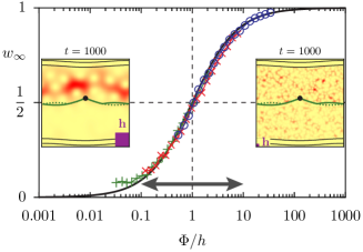
Figure 1: (Color online) Asymptotic transmitted weight $w_{\infty}$ vs. $\Phi/h$ for $\Phi\approx\frac{1}{3000}$ (pluses), $\frac{1}{800}$ (crosses), $\frac{1}{200}$ (circles), $h=\frac{1}{100},\dots,\frac{1}{6400}$ compared to Eq. (4) (solid line). Insets: Husimi representation of time-evolved wave packet for $\Phi\approx\frac{1}{200}$, $h=\frac{1}{40}$ and $h=\frac{1}{1000}$.

The quantum suppression of transport for $h\gg\Phi$ has consequences for the time evolution of a localized wave packet initially associated with a phase space region on one side of the partial barrier. It cannot acquire a substantial weight on the other side of the partial barrier even in the limit of arbitrarily large times; see Fig. 1 left inset. This is reflected in the eigenstates having much stronger projection in either one of the two sides; see Fig. 3 left insets. In contrast, for $h\ll\Phi$ wave packets in the long-time limit as well as eigenstates extend to both regions as if the partial barrier were not present. This corresponds to the classical behavior where in the long-time limit chaotic orbits explore both regions ergodically.

The quantum localizing transition between quantum suppression and classical transport has been studied theoretically and experimentally for multiphoton ionization of atoms MacKay and Meiss (1988), cesium atoms in optical potentials Vant et al. (1999), and microcavity lasers Shim et al. (2008); *YanLeeShiMooLeeKimLeeAn2008; *ShiHarFukHenSasNar2010; *ShiWieCao2011. The most extensive study goes back to Bohigas, Tomsovic, and Ullmo (BTU) on coupled quartic oscillators where seven chaotic regions are separated by six partial barriers Bohigas et al. (1993); *BohTomUll1990a; *SmiTomBoh1992. They model the quantum mechanism of a partial barrier by globally coupled random matrices with a transition parameter determined by $\Phi/\hbar$, which were previously used to describe symmetry breaking Rosenzweig and Porter (1960); *French88; *GuhWei1990. They found good agreement for the implications of partial barriers on spectral statistics and wave packet dynamics.

While the quantum localizing transition is partially understood, the full quantitative transition even for an isolated partial barrier so far is not. In particular one is interested in the transition curve, including its universal scaling, center, width, shape, and whether it has quantized steps. This is a prerequisite for understanding the critical essence in quantum mechanics of the turnstile.

In this paper we analyze the quantum localizing transition with the help of a designed quantum map with an isolated partial barrier of controllable flux $\Phi$. By studying wave packet dynamics and eigenstate properties, it is found that the transition from quantum suppression to classical transport is universal with the expected scaling parameter $\Phi/h$, is symmetric to $\Phi/h=1$, exhibits no quantized steps, and has a 10%-90% width of two orders of magnitude in $\Phi/h$; for simplicity the results presented are quoted for a system with only two regions, both of comparable phase space areas. It is shown that the critical essence in quantum mechanics of a turnstile is a local coupling mechanism in contrast to the previously used global coupling scheme. We give an analytical description of the universal transition based on a phenomenological $2\times 2$-model. The findings are confirmed with the more familiar standard map, which plays an important role in studies of quantum chaos and localization Casati and Ford (1979); *Fishman82.

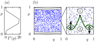
Figure 2: (Color online) (a) $T^{\prime}(p)$ of the designed map $F$ with $\Phi\approx\frac{1}{200}$. (b) Corresponding phase space with a large chaotic sea (dots) between the regular tori (lines) and zoom with hyperbolic fixed point (black circle), partial barrier (solid green line) separating regions 1 and 2, its preimage (dotted green line) and the turnstile areas of size $\Phi$.

Consider a family of designed area preserving maps $F$ of the two-torus, see Fig. 2 for an illustration. The phase space consists of a large chaotic sea between the regular tori. There is a hyperbolic fixed point at $(q,p)=(\frac{1}{2},{p}_{\text{fix}})$, whose stable and unstable manifold can be used to construct a partial barrier separating the regions 1 and 2 of approximately the same size, $A_{1}\approx A_{2}$. The region between the partial barrier and its preimage defines the turnstile areas of size $\Phi$ Meiss (1992). The map $F$ was designed such that this partial barrier is well isolated with a small tunable flux. This is achieved by a composition of two maps, $F=F_{\mathrm{rot}}\circ F_{\mathrm{kick}}$. Here $F_{\mathrm{kick}}$ originates from a kicked Hamiltonian and is given by $(q^{\prime},p^{\prime})=(q+T^{\prime}(p^{*}),p^{*}-V^{\prime}(q^{\prime})/2)$ using $p^{*}=p-V^{\prime}(q)/2$ with $V^{\prime}(q)=\sin(2\pi q)/(4\pi)$ and piecewise linear $T^{\prime}(p)$, see Fig. 2(a). In order to destroy additional partial barriers not related to the fixed point we use a map $F_{\mathrm{rot}}$, which rotates points inside a circular region in phase space specified by center, radius and rotation angle while points outside this region are unchanged Note1 . The parameters of $F_{\mathrm{kick}}$ and $F_{\mathrm{rot}}$ for the three considered cases of $F$ with fluxes $\Phi\approx\frac{1}{3000}$, $\frac{1}{800}$, and $\frac{1}{200}$ are given in Refs. Michler et al. ; Michler (2011). Quantum mechanically the system is described by a unitary operator $U=U_{\mathrm{rot}}U_{\mathrm{kick}}$ acting on a Hilbert space of finite size $N$ with effective Planck’s constant $h=1/N$. Here $U_{\mathrm{kick}}=\exp\{-\text{i}V({q})/(2\hbar)\}\exp\{-\text{i}T({p})/\hbar\}\exp\{-\text{i}V({q})/(2\hbar)\}$ and $U_{\mathrm{rot}}=U_{\text{ho}}P_{\text{ho}}+(\mathbf{1}-P_{\text{ho}})$ where $P_{\text{ho}}$ is a projector built from harmonic oscillator eigenstates within the rotating region and $U_{\text{ho}}$ gives the time evolution corresponding to the classical rotation angle Note1 . The time evolution of a wave packet $\psi(t)$ is given by $\psi(t+1)=U\psi(t)$.

In order to quantify the quantum transition of a partial barrier we define the (relative) asymptotic transmitted weight $w_{\infty}$ of a wave packet $\psi_{1}$ started in region 1 as

$$w_{\infty}[\psi_{1}] :=\frac{\langle\mu_{B_{2}}[\psi_{1}(t)]\rangle_{t}}{\mu^{\text{cl}}_{B_{2}}}.$$ (1)

It is the time-averaged transmitted weight divided by the corresponding classical weight $\mu^{\text{cl}}_{B_{2}}$. As initial state we choose $p_{0}=0.7$ and as a measure $\mu_{B_{2}}$ the probability of $\psi_{1}(t)$ within the region ${B_{2}}$ ($p\in[0.175,0.325]$). The classical weight $\mu^{\text{cl}}_{B_{2}}$ is the relative time a long chaotic orbit spends in ${B_{2}}$. Assuming ergodicity in the chaotic sea of size $A_{\text{ch}}$ it can be determined by $\mu^{\text{cl}}_{B_{2}}={{B_{2}}}/{A_{\text{ch}}}$. The definition of $w_{\infty}$ implies that it makes a transition from 0 for $h\gg\Phi$ to 1 for $h\ll\Phi$. In the latter case this happens because any initial state becomes uniformly distributed at large times as would a classical distribution of trajectories.

Figure 1 shows the resulting $w_{\infty}$ vs. $\Phi/h$ for three different fluxes $\Phi$, averaged over 100 values of the Bloch phase and 100 time steps after time $T=2^{20}$. All data sets fall on top of each other under this scaling, i.e. $\Phi/h$ is indeed the correct scaling parameter. We expect that the quantum localizing transition for any partial barrier follows the same universal curve as a function of $\Phi/h$. This expectation assumes that the relative volumes of regions 1 and 2 are of the same order and that the mixing time is much shorter than the dwell time. Figure 1 shows that on a logarithmic scale the transition is symmetric with respect to the point $\Phi/h=1$, $w_{\infty}=\frac{1}{2}$. Thus the transition point is reached when flux $\Phi$ and Planck’s constant $h$ are equal. The transition is found to be smooth with no indications for quantized steps at integer values of $\Phi/h$. By defining the transition region as the interval in $\Phi/h$ for which $w_{\infty}\in[0.1,0.9]$, the width is seen to be two orders of magnitude, indicated by the arrow in Fig. 1. The overall behavior of the transition is well described by the symmetric curve of Eq. (4), which results from a phenomenological $2\times 2$ matrix model, see below. For the smallest $\Phi/h$ (below 0.05) there is an upward trend of $w_{\infty}$ compared to the symmetric curve. We attribute this deviation to the effect of tunneling across the entire partial barrier, which occurs in addition to quantum transport through the turnstile region. This is left for future investigation.

Complementary to the time evolution of wave packets, consider properties of eigenstates of the quantum map. States are either contained in region 1 or in region 2 in the case of $h\gg\Phi$, see Fig. 3 left inset. For $h\ll\Phi$ the states extend over the whole chaotic region, see Fig. 3 top right inset. In addition there exist regular eigenstates localized on the invariant tori and scarred states, e.g. on the hyperbolic fixed point. We define the average eigenstate equipartition measure $\langle w_{12}\rangle$ by

$$\langle w_{12}\rangle :=\frac{1}{N_{\text{ch}}}\sum\limits_{j=0}^{N-1}\frac{\mu_{B_{1}}[\phi_{j}]}{\mu^{\text{cl}}_{B_{1}}}\frac{\mu_{B_{2}}[\phi_{j}]}{\mu^{\text{cl}}_{B_{2}}}$$ (2)

as the sum of the products of the relative weights of eigenstates $\phi_{j}$ in each measuring box ${B_{1}}$ ($p\in[0.675,0.825]$) and ${B_{2}}$ ($p\in[0.175,0.325]$) contained in regions 1 and 2, resp. The relative weight compares the measure $\mu_{B_{i}}[\phi_{j}]$ with the corresponding classical weight $\mu^{\text{cl}}_{B_{i}}$. Eigenstates which are almost zero in one of the regions give no contribution, while the contribution is 1 for eigenstates, which are almost equipartitioned. The prefactor $1/N_{\text{ch}}$ is chosen such that in the semiclassical limit $\langle w_{12}\rangle$ approaches 1, as in this limit all $N_{\text{ch}}=A_{\text{ch}}/h$ chaotic states contribute 1, while regular states give no contribution.

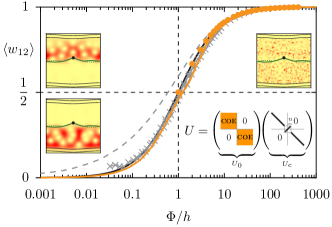
Figure 3: (Color online) Average eigenstate equipartition measure $\langle w_{12}\rangle$ for the designed map (gray crosses, same parameters as in Fig. 1) compared to Eq. (4) (solid line), the BTU model (gray dashed line) and the channel coupling model with discrete (orange circles) and continuous transmissions (light orange line) using 1000 realizations with $N_{1}=N_{2}=500$. Inset: Husimi representation of typical eigenstates for $\Phi\approx\frac{1}{200}$, $h=\frac{1}{40}$ (left) and $h=\frac{1}{1000}$ (top right). Illustration of the matrix structure of $U_{0}$ and $U_{\text{c}}$, where black lines represent unit entries (bottom right).

Figure 3 shows $\langle w_{12}\rangle$ for three different fluxes $\Phi$. One observes the same transitional behavior as for $w_{\infty}$, again well described by Eq. (4). In fact, one can show that $\langle w_{12}\rangle=\langle w_{\infty}[\psi_{1}^{k}]\rangle_{k}$ if $w_{\infty}$ is averaged over initial states $\psi_{1}^{k}$ which form an orthonormal basis in ${B_{1}}$.

In order to phenomenologically describe the transition we propose a unitary $2\times 2$ matrix model

$$U=\begin{pmatrix}\sqrt{1-v^{2}}&v\\ v&-\sqrt{1-v^{2}}\\ \end{pmatrix}.$$ (3)

Here the deterministic variable $v\in[0,1]$ describes the turnstile coupling between two sites representing the chaotic regions $A_{1}$ and $A_{2}$. Following from unitarity the diagonal entries have magnitude $\sqrt{1-v^{2}}$. The lower entry has a minus sign such that for $v=0$ the eigenvalues are not degenerate. The eigenvalues are $\pm 1$ independent of $v$ and the normalized eigenvectors are $\phi_{\pm}=1/\sqrt{2}(\pm c_{\pm},v/c_{\pm})$ with $c_{\pm}=\sqrt{1\pm\sqrt{1-v^{2}}}$. According to Eq. (2) the average eigenstate equipartition measure is $\langle w_{12}\rangle=v^{2}$, where the quantum measures $\mu_{B_{i}}[\phi_{\pm}]$ are given by the squared $i$-th element of the eigenvectors $\phi_{\pm}$ and the classical expectations are $\mu^{\text{cl}}_{B_{1}}=\mu^{\text{cl}}_{B_{2}}=\frac{1}{2}$. For the asymptotic transmitted weight $w_{\infty}$, Eq. (1), i.e. for a wave packet started on one site and measured on the other site, we find the same result, $w_{\infty}=v^{2}$. The parameter $v$ of this model can be related to the scaling parameter $\Phi/h$ of quantum maps with a partial barrier: We identify the transmission probability $v^{2}$ with the relative classical flux $\Phi/A_{i}$, i.e. $v^{2}=\Phi/A_{i}$. Moreover, we choose the Planck cell associated with each site of the $2\times 2$-model to be the sub-region of $A_{i}$ that is not transmitted, $h=A_{i}-\Phi$. This choice makes the regions associated with $h$ and $\Phi$ disjoint and thereby allows for arbitrary ratios of $\Phi/h$. This finally gives for the $2\times 2$-matrix model

$$w_{\infty} =\langle w_{12}\rangle=\frac{\displaystyle\Phi/h}{\displaystyle 1+\Phi/h}.$$ (4)

Quite amazingly this phenomenological model gives a very good description of the transitional behavior of the map data for the entire range from $\Phi/h\ll 1$ to $\Phi/h\gg 1$ (apart from the deviation for $\Phi/h\leq 0.05$ attributed to tunneling at small $\Phi/h$), see Figs. 1 and 3. This is reminiscent of the success of the Wigner surmise using $2\times 2$ matrices to describe universal spectral statistics. As no system specific properties were used in the derivation of Eq. (4), except for the scaling parameter $\Phi/h$, this gives further support for the universality of the transition curve. We expect that the universality also extends to time continuous Hamiltonian systems like billiards.

In order to get an insight into the quantum mechanism of a partial barrier we now study appropriately adapted random matrix models. In the BTU model Bohigas et al. (1993) two matrices of the Gaussian orthogonal ensemble, representing two chaotic regions, are globally coupled with a strength determined by $\Phi/h$. Figure 3 shows that for $\Phi/h<10$ this model overestimates the value of $\langle w_{12}\rangle$ found for the quantum map. We attribute this discrepancy to the global coupling of the BTU model. Instead we propose to model the classical turnstile mechanism by a local coupling via a channel. In a unitary model $U=U_{0}\cdot U_{\text{c}}$ we decompose the dynamics into a coupling matrix $U_{\text{c}}$ modeling the turnstile transport multiplied by an uncoupled matrix $U_{0}$ modeling the mixing in each of the regions 1 and 2, see Fig. 3 inset. The coupling matrix $U_{\text{c}}$ is an identity matrix, where the central $2n\times 2n$ block has ones on the anti-diagonal. It couples the two regions via $n$ modes for each direction of the channel. This models the directed transport of a turnstile in the classical system. The matrix $U_{0}$ is block diagonal consisting of two matrices of the circular orthogonal ensemble of sizes $N/2\times N/2$ and the limit of large $N$ is considered. This model has only one parameter, namely the number of modes $n=\Phi/h$. The resulting $\langle w_{12}\rangle$ for this unitary channel coupling model is shown in Fig. 3 and is in very good agreement with the numerical data of the map $F$. It is stressed that this agreement has been obtained without any fitting parameter. The model can be extended to non-integer values of $\Phi/h$ by the continuous transmissions of modes propagating through a channel Michler et al. , see Fig. 3. We observe that these models with local coupling are better describing the data for the map $F$ for $\Phi/h\leq 10$ compared to the global coupling BTU model and on the same level as the phenomenological $2\times 2$-model. This suggests that the turnstile mechanism of the classical system is quantum mechanically described by a local coupling via a channel.

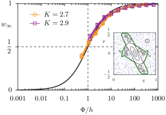
Figure 4: (Color online) Asymptotic transmitted weight $w_{\infty}$ using the Husimi measure for the standard map with $K=2.7$ ($\Phi\approx\frac{1}{200}$) and $K=2.9$ ($\Phi\approx\frac{1}{100}$) for $h=\frac{1}{100},\dots,\frac{1}{51200}$ versus $\Phi/h$ compared to Eq. (4) (solid line). The data is averaged over $15$ initial conditions placed in region 1, $10$ values of the Bloch phase, and $100$ time steps after time $10^{6}$. Data for four different variants Michler (2011); Michler et al. of the partial barrier are shown. Inset: One partial barrier (thick solid line) separating regions 1 and 2 for the standard map with $K=2.7$ as well as its preimage (dotted lines)

We now show results for the generic standard map, $(q^{\prime},p^{\prime})=(q+p,p+K\sin(2\pi q^{\prime})/(2\pi))$, with kicking strengths $K=2.7$ and $K=2.9$, where one has a dominant partial barrier separating two sufficiently large chaotic regions, see Fig. 4 inset and Ref. Michler et al. ; Michler (2011) for details. We consider the asymptotic transmitted weight $w_{\infty}$ of a wave packet initially located outside of the partial barrier in region 1. We integrate the Husimi function of the wave packet $\psi_{1}(t)$ over the measuring box ${B_{2}}$, which we choose as the entire region 2. Figure 4 shows good agreement of $w_{\infty}$ over the accessible range $\Phi/h\geq\tfrac{1}{2}$ with the universal behavior as observed in Figs. 1 and 3 and well described by Eq. (4).

We believe that the understanding of the universal behavior of the quantum localizing transition of an isolated partial barrier provides the building block to explain the power–law scaling Geisel et al. (1986); Grempel et al. (1984); Fishman et al. (1987) occurring in the presence of hierarchically organized partial barriers around a cantorus. Our results also open the possibility to tackle the tunneling regime which sets in for $\Phi/h\lesssim 0.1$. There in addition to the local channel coupling mechanism of the turnstile one has tunneling across the entire partial barrier. Finally, if an extended chaotic system has an infinite chain of well isolated partial barriers, then the classical dynamics is diffusive, and the quantum dynamics will lead to exponential localization no matter how open the partial barriers. This similarity to Anderson localization Anderson (1958) would be very interesting to explore based on the universal transition curve of quantum transport through a single partial barrier.