Block Iterative Eigensolvers for Sequences of Correlated Eigenvalue Problems

Abstract

In Density Functional Theory simulations based on the LAPW method, each self-consistent field cycle comprises dozens of large dense generalized eigenproblems. In contrast to real-space methods, eigenpairs solving for problems at distinct cycles have either been believed to be independent or at most very loosely connected. In a recent study [7], it was demonstrated that, contrary to belief, successive eigenproblems in a sequence are strongly correlated with one another. In particular, by monitoring the subspace angles between eigenvectors of successive eigenproblems, it was shown that these angles decrease noticeably after the first few iterations and become close to collinear. This last result suggests that we can manipulate the eigenvectors, solving for a specific eigenproblem in a sequence, as an approximate solution for the following eigenproblem. In this work we present results that are in line with this intuition. We provide numerical examples where opportunely selected block iterative eigensolvers benefit from the reuse of eigenvectors by achieving a substantial speed-up. The results presented will eventually open the way to a widespread use of block iterative eigensolvers in ab initio electronic structure codes based on the LAPW approach.

1 Introduction

Materials simulations based on Density Functional Theory [1] (DFT) methods have at their core a set of partial differential equations (Kohn-Sham [2]) which eventually lead to a non-linear generalized eigenvalue problem. Solving the latter directly is a daunting task and a numerical iterative self-consistent approach is preferred. It starts off by inputting an approximate electronic charge density to a cyclic process within which a linearized version of the eigenvalue problem is initialized and solved. At the end of each cycle a new charge density is computed and compared with the initial one. Self-consistency is reached when the distance between the input and output densities is below a certain required threshold; the process is then said to have converged. The entire simulation results in a series of so called “outer-iteration cycles” often referred to as self-consistent field iterations.

Roughly speaking, all the existing DFT-based methods differ from each other by the choice of linearization scheme (also denoted as discretization), and by the choice of the effective Kohn-Sham (KS) potential. There are three discretization strategies commonly in use: 1) manipulation of localized functions (Gaussians, etc.), 2) expansion of the eigenfunctions over a plane wave basis set, and 3) discretization of the KS equations over a lattice in real space. While the first method is almost exclusively used in Quantum Chemistry the last two are widely used in Materials Science and present a series of pros and cons. The plane wave expansion leads to Hamiltonians with kinetic energy terms only on the main diagonal and are well suited to simulate solid crystals. In turn this discretization needs to approximate the Coulomb potential near the nuclei substituting it with a smooth pseudo-potential. In real-space discretization, potential terms in the Hamiltonian decay exponentially away from the diagonal [6] giving rise to quite sparse and large eigenvalue problems. This strategy is well suited mostly for disordered systems and insulators.

Among the plane wave strategies, the Full-Potential Linearized Augmented Plane Wave (FLAPW)  [4, 5] method constitutes one of the most precise frameworks for simulating transition metals and magnetic systems. The Kohn-Sham equations are discretized using a mix of radial and plane wave functions (see section 2), parametrized by a vector k within the Brillouin zone of the momentum lattice. At each outer-iteration $\ell$ a set of eigenpencils $P^{(\ell)}_{\bf k}$, labeled by k, is initialized and solved. Because FLAPW uses full-potential together with a partial plane wave expansion, each $P^{(\ell)}_{\bf k}$ is a dense and hermitian generalized eigenvalue problem; its size $n$ depends linearly – with a large pre-factor – on the number of atoms considered in a simulation, and typically ranges between 2,000 and 20,000. Only a relatively small percentage of the bottom end of the spectrum is required, never exceeding 15-20%, and often quite less.

In this work we consider sequences of generalized hermitian eigenvalue problems as they arise in FLAPW. In this context a sequence is a set of $N$ generalized eigenproblems identified by a progressive index $\ell$

$$\{P^{(\ell)}\}\doteq P^{(1)},\dots,P^{(N)}\qquad;\qquad P^{(\ell)}:\quad A^{(\ell)}x=\lambda\ B^{(\ell)}x.$$ (1)

Within a sequence each eigenproblem is characterized by a hermitian indefinite matrix $A$ and a positive definite hermitian matrix $B$. This setup is generally referred to as a matrix pencil or eigenpencil and it is known to have a bounded discrete spectrum with real positive and negative eigenvalues

$$\lambda_{\rm min}=\lambda_{1}\leq\lambda_{2}\leq\dots\leq\lambda_{n}=\lambda_{\rm max}.$$ (2)

Eigenpencils usually admit $n$ distinct eigenvectors $x_{i}$ satisfying a $B$-orthonormality relation $(x_{i},Bx_{j})=\delta_{ij}$ even when they correspond to identical eigenvalues. While in general $B\neq I$, in the special case $B=I$ the eigenpencil becomes a standard eigenvalue problem, and the orthonormality relation reduces to the standard $(x_{i},x_{j})=\delta_{ij}$.

In current codes implementing FLAPW [18, 19, 20, 21, 22], each sequence of eigenpencils $\{P^{(\ell)}\}$ is handled very much as a set of uncorrelated problems: each $P^{(\ell)}$ is solved in complete isolation from any other and independently passed as input to a prepackaged eigensolver of a standard library – like LAPACK [23] or its parallel version ScaLAPACK [24] – which outputs the desired portion of eigenspectrum and corresponding eigenvectors. The eigensolver is thus used as a black box and has no knowledge of the eigenproblems’ spectral properties nor of the application from which they originated. As much as this process grants standardization and reliability, it is also far from being optimal. What is “lost in translation” is the possibility to render manifest the correlation between eigenpencils of the sequence $\{P^{(\ell)}\}$ in terms of precise numerical properties which are then passed to a solver that can exploit them.

In a recent work [7] it has been reported that eigenpencils with a successive outer-iteration index $\ell$ and the same k-vector are strongly correlated. Consequently, problems in a sequence are not only connected by a progressive index but, as for a sequence of numbers, there is a relation linking them. In FLAPW, such a numerical correlation become evident in the way the subspace angles between eigenvectors evolve from larger to smaller values as the sequence progresses towards higher outer-iteration indices [7]. It needs to be stressed that, contrary to what happens in real-space methods, the correlation between eigenvectors is a new and unexpected feature of FLAPW-based methods: since the eigenfunctions are delocalized and the function basis set is modified at each successive outer-iteration, it had been common belief that correlation was an unlikely phenomenon.

With evidence of the contrary in hand, it becomes natural to consider eigenvectors of $P^{(\ell)}$ as a set of approximate solutions that can be used by an appropriate eigensolver to accelerate the solution of $P^{(\ell+1)}$. The novelty of our contribution consists in showing that, by exploiting the collinearity between vectors of adjacent problems, we can significantly improve the performance of certain classes of eigensolvers. Since no eigensolver (QR, MRRR, Divide&Conquer, etc.) for dense problems accepts as input approximate eigenvectors, our strategy can only be carried out by using iterative eigensolvers. In the rest of the paper we first illustrate, through numerical experiments, the success of this strategy for three distinct block iterative eigensolvers, each representing a specific class of available methods. Then we focus on one of these solvers, develop a C language version and obtain similar results with emphasis on high-performance and scalability.

In section 2 we first give a short description of how sequences of eigenproblems arise in DFT and how they translate into apparently uncorrelated dense eigenvalue problems. We then proceed to briefly report on the correlation between adjacent eigenproblems as illustrated in [7]. Our core results are presented in section 3 where we introduce the selected block iterative eigensolvers followed by a description of the experimental setup and the numerical tests performed. We summarize our results in section 4, and conclude with future work and acknowledgments.

2 Sequences of correlated eigenproblems

In this section we illustrate in some detail how sequences of eigenpencils arise in DFT. We start with a brief recall of the fundamentals of quantum mechanics, explain the need for an effective theory dealing with many particles and describe the FLAPW method self-consistent cycle. It is then shown why correlation among eigenproblems in a sequence is unexpected, and how the presence of such a correlation was exposed by looking at the evolution of eigenvectors as a function of the outer-iteration cycle index $\ell$.

2.1 The rise of sequences in Density Functional Theory

The electronic structure of a quantum mechanical system with $L$ atoms and $M$ electrons is described by the Schrödinger equation

$$H\,\Phi(x_{1};s_{1},\dots,x_{n};s_{n})=\mathcal{E}\,\Phi(x_{1};s_{1},\dots,x_{n};s_{n}).$$ (3)

$H=-\frac{\hbar^{2}}{2m}\sum_{i=1}^{M}\nabla^{2}_{i}-\sum_{i=1}^{M}\sum_{\mu=1}^{L}\frac{Z_{\mu}}{|x_{i}-a_{\mu}|}+\sum_{i<j}\frac{1}{|x_{i}-x_{j}|}$ is the Hamiltonian characterizing the dynamics of the electrons whose positions and spins are indicated by $x$ and $s$ respectively. $\mathcal{E}$ represents the energy of the system while $\Phi$ is the high-dimensional antisymmetric electronic wave function solving for eq. (3). Already at this stage the Schrödinger equation looks very much like an eigenvalue problem, unfortunately one that is already very challenging to solve for values $M,L\geq 2$.

During the 1960s, a series of simplifications were introduced based on rigorous theorems [2, 3] where the exact high-dimensional eq. (3) was replaced by a large set of one-dimensional Kohn-Sham equations

$$\forall\ a\quad\textrm{solve}\quad\hat{H}_{\rm KS}\phi_{a}({\bf r})=\left(-\frac{\hbar^{2}}{2m}\nabla^{2}+V_{0}({\bf r})\right)\phi_{a}({\bf r})=\epsilon_{a}\phi_{a}({\bf r}).$$ (4)

The most important element in these equations is the substitution of the last two terms of $H$ with an effective potential $V_{0}({\bf r})[n]$ that functionally depends on the charge density $n({\bf r})$: a function of all the one-particle wave functions $\phi_{a}({\bf r})$. Because of this interdependence between $V_{0}$ and $\phi_{a}({\bf r})$, eq. (4) constitutes a set of non-linear partial differential equations.

Typically this set of equations is solved using an outer-iterative self-consistent cycle: it starts off with an initial charge density $n_{init}({\bf r})$, proceeds through a series of iterations and converges to a final density $n_{N}({\bf r})$ such that $|n^{(N)}-n^{(N-1)}|<\eta$, with $\eta$ as an a priori parameter. Convergence is achieved by an oppurtune mixing between output density $n_{i}({\bf r})$ and one or more previous input densities $n_{\ell<i}({\bf r})$. In the particular case of FLAPW the new density is computed by a quasi-Newton mixing with the inverse Jacobian updated by Broyden’s second method [25, 26].

$$\begin{array}[l]{ccc}\color[rgb]{1,0,0}{\framebox{\rule[-5.69046pt]{0.0pt}{17.07182pt}\shortstack{{\small Initial input}\\ $n_{\rm init}({\bf r})$}}}&&\\[11.38109pt] \Downarrow&&\\[5.69054pt] \framebox{\rule[-5.69046pt]{0.0pt}{17.07182pt} \shortstack{{\small Compute KS potential}\\ $V_{0}({\bf r})[n]$}}&\longrightarrow&\framebox{\rule[-5.69046pt]{0.0pt}{17.07182pt} \shortstack{{\small Solve KS equations}\\ $\hat{H}_{\rm KS}\phi_{a}({\bf r})=\epsilon_{a}\phi_{a}({\bf r})$}}\\[11.38109pt] \uparrow{\rm No}&&\downarrow\\[5.69054pt] \framebox{\rule[-5.69046pt]{0.0pt}{17.07182pt} \shortstack{\small Converged? \\ $|n^{(\ell+1)}-n^{(\ell)}|<\eta$}}&\longleftarrow&\framebox{\rule[-5.69046pt]{0.0pt}{17.07182pt} \shortstack{{\small Compute new density}\\ $n({\bf r})=\sum_{a}|\phi_{a}({\bf r})|^{2}$}}\\[11.38109pt] \Downarrow\textrm{Yes}&&\\[11.38109pt] \color[rgb]{0,0,1}{\framebox{\rule[-5.69046pt]{0.0pt}{17.07182pt} \shortstack{{\small OUTPUT}\\ {\small Energy, forces, etc.}}}}&&\end{array}$$ (5)

In practice this outer-iterative cycle is still quite computationally challenging and requires some form of broadly defined discretization. In the FLAPW method, the wave functions $\phi_{a}({\bf r})$ are expanded on a basis set $\psi_{\bf G}({\bf k},{\bf r})$ parametrized by vectors k living in the momentum space discretized on a lattice

$$\phi_{a}({\bf r})\longrightarrow\phi_{{\bf k},\nu}({\bf r})=\sum_{|{\bf G+k}|\leq{\bf K}_{max}}c^{\bf G}_{{\bf k},\nu}\psi_{\bf G}({\bf k},{\bf r}).$$ (6)

Here ${\bf K}_{max}$ is a cut-off and its value determines the range of the vector index ${\bf G}$, ultimately controlling the size of the eigenproblems $n$ (not to be confused with the charge density n(r)). Thus, the number of basis functions in the expansion equals the size of the problem at hand. In FLAPW the basis functions $\psi_{\bf G}({\bf k},{\bf r})$ are constructed by merging together radial-like functions $u^{\alpha}_{\it l}(r)$ inside a spherical region around the atoms (also called Muffin-Tin) and simple plane waves in the interstitial areas between atoms

$$\psi_{\bf G}({\bf k},{\bf r})=$$

$$= \left\{\begin{array}[l]{l}\frac{1}{\sqrt{\Omega}}e^{i({\bf k+G}){\bf r}}\qquad\qquad\qquad\qquad\qquad\quad-\textrm{Interstitial}\\ \displaystyle\sum_{\it l,m}\left[a^{\alpha,{\bf G}}_{\it lm}({\bf k})u^{\alpha}_{\it l}(r)+b^{\alpha,{\bf G}}_{\it lm}({\bf k})\dot{u}^{\alpha}_{\it l}(r)\right]Y_{\it lm}(\hat{\bf r}_{\alpha})\hfill-\textrm{MT}.\\ \end{array}\right.$$

At each iteration cycle the radial functions are computed anew by solving auxiliary Schrödinger equations. Moreover a new set of the coefficients $a^{\alpha,{\bf G}}_{\it lm}$ and $b^{\alpha,{\bf G}}_{\it lm}$ is derived by imposing continuity constraints on the surface of the Muffin-Tin spheres. Consequently at each iteration the basis set $\psi_{\bf G}({\bf k},{\bf r})$ changes entirely. As will be explained in the next section, this peculiarity of the FLAPW method is one of the main reasons why correlation between eigenvectors of adjacent eigenproblems had been, until recently, considered unlikely.

Having defined a basis set of wave functions allows us to translate the KS equations into a set of generalized eigenvalue problems. First the expression (6) is inserted in eq. (4)

$$\psi^{*}_{\bf G}({\bf k},{\bf r})\sum_{\bf G^{\prime}}\hat{H}_{\rm KS}\ c^{\bf G^{\prime}}_{{\bf k},\nu}\ \psi_{\bf G^{\prime}}({\bf k},{\bf r})=\lambda_{{\bf k}\nu}\ \psi^{*}_{\bf G}({\bf k},{\bf r})\sum_{\bf G^{\prime}}c^{\bf G^{\prime}}_{{\bf k},\nu}\ \psi_{\bf G^{\prime}}({\bf k},{\bf r}).$$ (8)

Then, by integrating the left and right hand side of eq. (8) over the configuration space, the matrix entries for the Hamiltonian $A_{\bf k}$ and Overlap matrices $B_{\bf k}$ are computed

$$\left[A_{\bf k}\,\,B_{\bf k}\right]_{\bf GG^{\prime}}=\sum_{\alpha}\int d{\bf r}\ \psi^{\ast}_{\bf G}({\bf k},{\bf r})\left[\hat{H}_{\bf KS}\,\,\hat{\mathbb{1}}\right]\psi_{\bf G^{\prime}}({\bf k},{\bf r}).$$ (9)

The end result is a set of generalized eigenvalue equations parametrized by the vector k

$$P_{\bf k}:\quad\sum_{\bf G^{\prime}}(A_{\bf k})_{\bf GG^{\prime}}\ c^{\bf G^{\prime}}_{{\bf k}\nu}=\lambda_{{\bf k}\nu}\sum_{\bf G^{\prime}}(B_{\bf k})_{\bf GG^{\prime}}\ c^{\bf G^{\prime}}_{{\bf k}\nu}\hfill\,\,\equiv\,\,A_{\bf k}x_{i}=\lambda_{i}B_{\bf k}x_{i}.$$

As can be readily seen the coefficients $c_{{\bf k}\nu}$ play the role of eigenvectors while the indices ${\bf k}$ and $\nu$ can be compactly condensed in the single index $i$. Moreover because of the complex structure of $\psi_{\bf G}({\bf k},{\bf r})$, interactions in $\hat{H}_{\bf KS}$ are “delocalized” with the net effect of filling up the Hamiltonian matrix $A$ and losing any diagonal dominance. At the same time the over-completeness of the basis set renders $B$ dense as well as somewhat ill-conditioned. These characteristics differentiate FLAPW-based methods from real-space ones, and make them very well suited to simulate physical systems where electrons are partially delocalized (metals, semi-conductors, etc.).

The net effect of this discretization is the translation of the KS equations into a set of generalized eigenvalue problems for each outer-iteration

$$\begin{array}[l]{ccc}\framebox{\rule[-5.69046pt]{0.0pt}{17.07182pt} \shortstack{{\small Solve KS equations}\\ $\hat{H}_{\rm KS}\phi_{a}({\bf r})=\epsilon_{a}\phi_{a}({\bf r})$}}&\Rightarrow&\framebox{\rule[-5.69046pt]{0.0pt}{17.07182pt} \shortstack{{ Solve a set of eigenproblems}\\ $P_{{\bf k}_{1}}\dots P_{{\bf k}_{N}}$}}.\end{array}$$

In the end the entire process has at its core the initialization and solution of a set of sequences of dense eigenpencils $\{P^{(\ell)}_{\bf k}\}$.

2.2 Correlation in the sequence

In analogy to the definition of a sequence of numbers, a sequence of eigenvalue problems is considered as such if $P^{(\ell)}$ has some connection to $P^{(\ell+1)}\ \forall\ell$. Therefore, we now focus on a single sequence $\{P^{(\ell)}\}$ and describe how this correlation becomes manifest in the evolution of subspace deviation angles between eigenvectors of successive eigenproblems.

In sequences arising from DFT the most obvious form of connection comes from the fact that the problem with index $\ell+1$ is initialized only after the previous problem is solved. Despite this simple fact, the initialization and solution of the new eigenproblem depends very indirectly on the solution of the old one. Eq. (9) shows that matrix entries are computed using a new set of $\psi^{(\ell+1)}_{\bf G}({\bf k},{\bf r})$, whose Muffin-Tin (MT) components can be radically different from the one of $\psi^{(\ell)}_{\bf G}({\bf k},{\bf r})$. The same MT components depend very non-linearly on the charge density ${\it n}({\bf r})$ which, in turn, is a sum of linear combinations (see eq. (6)) of eigenvectors $c^{(\ell)}_{{\bf k}\nu}$ and the same basis functions $\psi^{(\ell)}_{\bf G}({\bf k},{\bf r})$. In conclusion at each outer-iteration, the Hamiltonian, the Overlap and the basis function set vary substantially and in a way that cannot be estimated. Due to this series of deductions, the correlation between successive eigenvalue problems in FLAPW is a rather novel discovery which had been considered by the computational physics community to be a rather unlikely outcome.

In [7] the link between adjacent eigenproblems is unraveled by looking at the existence of a correlation between eigenvectors as a numerical inverse problem. Starting from a constrained assumption, the authors conduct an a posteriori numerical analysis of angles between eigenvectors with successive outer-iteration indices $\ell$. For instance, let us look at two neighboring eigenproblems of a sequence

$$A^{(\ell)}x^{(\ell)}=\lambda\ B^{(\ell)}x^{(\ell)}\quad{\rm and}\quad A^{(\ell+1)}x^{(\ell+1)}=\lambda\ B^{(\ell+1)}x^{(\ell+1)},$$

with $B^{(\ell)}=L^{(\ell)}\ L^{(\ell)T}$ and $B^{(\ell+1)}=L^{(\ell+1)}\ L^{(\ell+1)T}$ the Cholesky decomposition of the respective Overlap matrices. In [7] it is shown that the eigenvectors of these two problems satisfy the following general relation

$$\langle x^{(\ell)}_{i}x^{(\ell+1)}_{j}\rangle= \ c^{*(\ell)}_{{\bf k},\nu}L^{(\ell)}\ L^{(\ell+1)T}\ c^{(\ell+1)}_{{\bf k},\mu}$$ (10)

$$= \ \delta_{ij}+\varepsilon\left[E_{ij}-c^{*(\ell)}_{{\bf k},\nu}\ L^{(\ell)}\ D\ L^{(\ell+1)T}\ c^{(\ell+1)}_{{\bf k},\mu}\right]+o(\varepsilon^{2}),$$

where both $E$ and $D$ are block diagonal, each block being diagonally dominant, and $\varepsilon$ being an expansion parameter. As long as $\varepsilon$ is small, eq. (10) implies that the matrix of scalar products between eigenvectors of adjacent eigenproblems has a lumpy structure with most of its dominant entries concentrated in the neighborhood of the main diagonal. This structure makes it possible to devise an algorithm establishing a one-to-one association between a generic eigenvector $x^{(\ell)}_{i}$ of $A^{(\ell)}$ and the corresponding eigenvector $x^{(\ell+1)}_{i}$ of $A^{(\ell+1)}$.

Once established, the one-to-one correspondence lays the ground for a systematic numerical analysis of the distribution of deviation angles $\theta^{(\ell)}_{i}=\langle x^{(\ell)}_{i}x^{(\ell+1)}_{i}\rangle$ along the entire sequence. Plots of $\theta^{(\ell)}_{i}$ illustrate how the eigenvectors become more and more collinear as the sequence progresses (e.g. Figure 1). In particular, we can observe how angles are already very small – $\sim$ 10^-4 on average – after a few iterations, becoming almost negligible towards the end of the self-consistent cycle. This result confirms a posteriori the correctness and reliability of the expansion (10) in powers of $\varepsilon$.

The importance of the eigenvector collinearity is two-fold: on the one hand it makes it clear that there is a deep connection between the convergence of the charge density $n({\bf r})$ and the solutions of the eigenpencils. At the same time it provides the means to go beyond the current algorithmic paradigm so as to improve the solving process of the entire sequence.

Table 1: Simulation data

Materials	nev	Kmax	# of iterations	Size of eigenproblems
CaFe2As2	136	4.0	24	2,612
Au98Ag10	972	3.0	22	5,638
		3.5	29	8,970
Na15Cl14Li	256	3.0	13	3,893
		3.5	13	6,217
		4.0	13	9,273

We will see in the next section how this is possible for a selected group of iterative eigensolvers. We conclude this section by illustrating two examples of evolution of deviation angles taken from real case solid-state crystals: CaFe₂As₂ and Au₉₈Ag₁₀. The first is a superconducting compound that undergoes a first order phase transition from a high temperature tetragonal phase to a low temperature orthorhombic phase. The latter is an artificial alloy of gold and silver. In order to avoid cluttering, in Figure 1 $\theta^{(\ell)}_{i}$ are plotted only for a small fraction of the eigenspectrum. In both plots, we can observe the deviation angles decreasing quasi-monotonically during the entire sequence. This behavior is not only characteristic of the lowest portion of the spectrum; it is noticed for all values of the index $i$. Simulation data for these two materials are shown in Table 1.

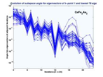
(a) Lowest 3% of eigenspectrum for CaFe₂As₂.

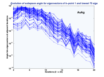
(b) Lowest 1.5% of eigenspectrum for Au₉₈Ag₁₀.

Figure 1: Evolution of subspace deviation angles between eigenvectors of adjacent eigenvalue problems within a sequence.

3 Exploiting the sequence evolution

In the following we present experimental evidence of the acceleration of iterative eigensolvers due to the use of approximate solutions. We proceed in two stages: first, using a direct eigensolver, we compute the eigenpairs of eigenpencil $P^{(\ell)}$ for a certain fraction of the eigenspectrum. Next, we feed these eigenpairs to a selected iterative eigensolver as an initial guess when solving for $P^{(\ell+1)}$. Finally we repeat the same computation with randomly generated vectors and compare the respective CPU times. These tests are repeated for three different choices of crystals and at each increasing outer-iteration index. The result of the comparison provides a measure of the possible speed-up iterative methods can achieve when used in sequences of correlated eigenvalue problems.

Among the many available iterative methods, only a few possess the ability of taking advantage of multiple approximate solutions and gain a sensible speed-up. In this respect an iterative algorithm has to comply with two essential properties: 1) the ability to receive as input a sizable set of approximate eigenvectors, and 2) the capacity to solve simultaneously for a substantial portion of eigenpairs. In particular we considered three classes of iterative eigensolvers: Davidson, conjugate gradient and subspace iteration. Krylov subspace methods [8, 9] were not included due to their inability to even converge all the requested eigenpairs without incurring in “stalled” computations. For each class we choose a block eigensolver whose characteristics are the closest to the requirements listed above. Block methods generalize the action of an eigensolver on one single approximate eigenvector to a set of vectors. As such they satisfy quite clearly the first requirement while the ability to obtain multiple eigenpairs in one shot is rather algorithm dependent.

In this section two sets of numerical results are illustrated: first we test three iterative algorithms exclusively in a Matlab environment. The objective is to gain an overview of the behavior of the eigensolvers and their relative efficiency in exploiting approximate solutions. In a second moment we focus on one of the eigensolvers, briefly illustrate its implementation in the C programming language and conduct a more performance-oriented numerical analysis of its features. In section 3.1 we illustrate the salient characteristics and properties of the block algorithms under scrutiny. This is followed by a detailed description of the experimental setup. Finally in section 3.3 the results of our numerical tests are presented and explained.

3.1 Block iterative eigensolvers

By their own nature iterative eigensolvers come in many variants and often some of their internal parameters can be tuned opportunely. In block methods one obvious input parameter is the block size blk; since block methods are notoriously more efficient in dealing with multiple and clustered eigenvalues, adjusting blk could improve the eigensolver performance. On the other hand, knowing a priori the positions of clusters of eigenvalues is usually not possible, so a value of blk that is optimal for a certain fraction of eigenspectrum may not work for another. On algorithms augmented with a polynomial accelerator another evident parameter is the polynomial degree deg. In this case a good choice for deg would balance the influence of two competing mechanisms: CPU time spent in performing matrix-matrix operations and the efficiency with which vectors converge to the solution.

In light of these considerations, it is important to understand that an eigensolver that performs well for a certain problem may become very slow for another. In particular we want to stress that we utilize iterative eigensolvers outside the “comfort zone” where they usually perform the best, namely sparse eigenproblems. By using these solvers on dense eigenproblems we are deliberately pushing them to the limit. The idea is to compensate for the misuse of the solvers by providing them with approximate eigenvectors. In doing so we want to test how effectively each eigensolver can gain in performance by exploiting problem solutions of the previous outer-iteration.

In order to extract the best behavior, all the numerical tests were carried out after optimizing each solver to the specific problem at hand. Such an optimization was achieved by tuning the values of the available parameters (see table 3). Despite these efforts not all eigensolvers seemed to have been able to take full advantage of the approximate solutions. We emphasize that this behavior is in no way detrimental to the value of the particular solver; it just indicates that the chosen eigensolver was too stressed to be able to overcome the inherent difficulties of the dense eigenproblems selected. All the eigensolvers described below were inherently developed for the lower portion of the spectrum. Unless otherwise specified, in the rest of the paper we refer exclusively to this part of the eigenspectrum.

Block Chebyshev-Davidson (BChDav) – This eigensolver is part of the Davidson-like methods. These methods sacrifice the Krylov subspace structure by computing an approximate residual which, opportunely preconditioned, is used to augment the subspace. In 2007 Saad and Zhou developed a version of the Davidson algorithm for problems where the preconditioning could be unknown or too expensive to compute [11]; in particular by filtering with Chebyshev polynomials the augmentation vector instead of solving a correction equation, they achieve better numerical results.

In 2010 Zhou implemented a block version of this method by adding an inner restart loop beside the usual outer restart one [12]. This version of the method succeeds in better deflating converged vectors and has the added ability to accept approximate solutions in place of the standard augmentation vectors. In particular the inner restart loop allows the addition of a new block of approximate vectors as soon as some of the sought after eigenpairs have converged. This is the first of the Chebyshev filtered methods that we tested. In his work Zhou has also shown that the method is not particularly sensitive to blk nor to deg. In our test we verified that this is indeed true and fairly small variations in computing time are observed by varying one or both of the parameters independently of the size of the eigenproblem. For our test we used a Matlab version of BChDav kindly provided by Y. Zhou.

Locally optimized block preconditioned conjugate gradient (Lobpcg) – Developed in 2001 by Knyazev [13], this algorithm uses a locally optimized version of a three-term recurrence relation for the preconditioned conjugate gradient method. In practice the Rayleigh-Ritz method is used for the eigenpencil on a trial subspace generated by the current guess for the Ritz vector, the preconditioned residual, and a third Ritz vector built by maximizing the Rayleigh quotient. Knyazev implemented a block version of the algorithm where the three-term relation is generalized for a block of vectors.

We performed our tests using the freely available Matlab version of the code. In this version blk is set by construction to be equal to the number of requested eigenpairs nev. While this choice seems natural, it encounters difficulties in converging the last few vectors requested due to the reduced size of the trial subspace. Despite being potentially disruptive, this limit is usually overcome by setting a rather large tolerance for the residuals and restarting the solver with the obtained solutions and a smaller tolerance. In order to put this method on par with the others analyzed, we augmented blk by 5% of nev and introduced a slight modification in the stopping criterion. In this way we could use the eigensolver in one run and obtain solutions possessing the required accuracy.

We deliberately used this method without a preconditioner, since in general such an operator is unknown in DFT-generated sequences $\{P^{(\ell)}\}$. Moreover Lobpcg accepts the matrices of a generalized eigenproblem directly as input. We show that for the case of FLAPW-generated eigenproblems this is a sub-optimal use of the solver due to the high conditioning number of the overlap matrices $B$. Much better behavior is observed when the generalized eigenproblems are reduced to standard form and then inputted to the eigensolver (see Table 2).

Chebyshev filtered subspace iteration (ChFSI) – This is the second of the Chebyshev-filtered methods we tested. This method is well known in the literature [9] and has been developed in the context of Density Functional Theory in real-space by Chelikowsky et al. [14, 15] for the PARSEC code [27]. Subspace iteration is perhaps one of the oldest known iterative algorithms. This is by nature a block solver since it simply tries to build an invariant eigenspace by block-multiplying a set of vectors with the operator to be diagonalized. It is well known that this class of methods converges very slowly and could end up with blocks of vectors spanning an invariant eigenspace that are linearly dependent (rank deficient case). By using a polynomial filter on the initial set of blk vectors both these problems are improved very efficiently and the method experiences a high rate of acceleration.

Also in this case the degree of the filter deg does not particularly influence the convergence as long as it is sufficiently high. In general the value for blk is chosen to be bigger than the requested number of eigenpairs nev. This choice ensures that the last eigenpairs converge quickly enough. In ChFSI, the subspace iteration loop is preceded by a Lanczos step in order to determine the boundaries of the interval out of which the set of vectors is filtered.

Starting from the backbone of a routine first developed for a Matlab version of the PARSEC code, we implemented a more sophisticated algorithm including an inner loop and a natural “deflation and locking” mechanism for the converged eigenvectors. Contrary to the code used in PARSEC, our implementation performs several filtering steps until all eigenpairs have converged to the required tolerance. A more detailed description of the routine is provided in Algorithm 1 below.

Algorithm 1 Chebyshev Filtered Subspace Iteration with locking

1:Matrix $H^{(\ell)}$ of the standard problem, approximate eigenvectors $\hat{Y}:=\left[\hat{y}^{(\ell-1)}_{1},\ldots,\hat{y}^{(\ell-1)}_{{\tt blk}}\right]$ and eigenvalues $\lambda^{(\ell-1)}_{1}$ and $\lambda^{(\ell-1)}_{{\tt blk}+1}$

2:Wanted eigenpairs $\left(\Lambda,Y\right).$

3:

4:Estimating upper bound for the largest eigenvalue $\triangleright$ Lanczos

5:Repeat

6:     Filtering the vectors $\hat{Y}=C_{{\tt deg}}(\hat{Y}).$ by a deg Chebyshev polynomial $\triangleright$ Chebyshev filter

7:     Re-Orthonormalizing $\hat{Y}.$ $\triangleright$ Rayleigh-Ritz (Start)

8:     Compute the Rayleigh quotient $G=\hat{Y}^{\dagger}H^{(\ell)}\hat{Y}$

9:     solve the reduced standard problem $Gw=\lambda w$ giving $\big{(}\hat{\Lambda},\hat{W}\big{)}.$

10:     Compute new $\hat{Y}=\hat{Y}\hat{W}.$ $\triangleright$ Rayleigh-Ritz (End)

11:     for $i=\textrm{converged}\to\textsc{nev}$  do $\triangleright$ Deflation & Locking (Start)

12:         if $\cfrac{||H^{(\ell)}\hat{Y}(:,i)-\hat{\Lambda}(i)\hat{Y}(:,i)||}{||\hat{Y}(:,i)||}<\textsc{tol}$ then Checking residuals of Ritz vectors.

13:              $\Lambda\leftarrow\left[\Lambda\;\hat{\Lambda}(i)\right]$ Locking converged eigenpairs.

14:              $Y\leftarrow\left[Y\;\hat{Y}(:,i)\right]$

15:         else

16:              break

17:         end if

18:     end for$\triangleright$ Deflation & Locking (End)

19:     converged $\leftarrow i$

20:     $\hat{\Lambda}\leftarrow\left[\hat{\Lambda}(\textsc{converged}:\textsc{end})\right]$

21:     $\hat{Y}\leftarrow\left[\hat{Y}(:,\textsc{converged}:\textsc{end})\right]$

22:Until  converged $<$ nev

3.2 Experimental setup

In order to test the behavior of the selected solvers, we singled out sequences of eigenproblems arising from three DFT systems presenting heterogeneous physical properties: a metal, an ionic crystal and a high-temperature superconductor. Besides having different physical properties, these systems differ in the size of the eigenpencils, and in the structure of the eigenspectrum. Since the efficiency of iterative eigensolvers is often quite sensitive to these characteristics, we could verify the robustness of our conclusions in different conditions. Simulation data are collected in Table 1.

Each sequence $\{P^{(\ell)}\}$ of eigenproblems was generated by running simulations using FLEUR, a FLAPW-based code developed in Jülich [18]. By fixing a specific k-vector we identified one sequence per system and stored the relative $A^{(\ell)}$ and $B^{(\ell)}$ matrices. For all the simulations we adopted the value $\eta<$1e-03 (see eq. (5)) as a signal for convergence; in turn this choice determines the maximum value of the iteration index for each sequence. All simulations were run on JUROPA, a powerful cluster-based computer operating in the Supercomputing Centre of the Forschungszentrum Jülich.

The first set of numerical tests was performed using Matlab, version R2011b (7.13.0.564) under an OpenSuSE 12.1, running on two Intel i7-870 (Nehalem “Lynnfield”) quad-core processors at 2.93 GHz. In order to avoid lengthy simulations, we took advantage of Matlab multi-threaded routines so that up to four cores and 8 Gb of RAM (2 DDR3, 1333 MHz) were fully dedicated to computations. The second set of tests for the C language implementation of ChFSI was performed on one node of JUROPA equipped with 2 Intel Xeon X5570 (Nehalem-EP) quad-core processors at 2.93 GHz and 24 GB memory (DDR3, 1066 MHz). All CPU times were measured by running each test for each algorithm 12 times and taking the median of the results.

Directly solving for the generalized eigenproblems makes a fair comparison among the selected eigensolvers cumbersome. One of the solvers can use $B$ directly (i.e. Lobpcg) while the other two deal with generalized eigenproblems by left multiplying $B^{-1}$ to $A$. Unfortunately, because of the over-completeness of the set of basis functions in eq. (6), the overlap matrices $B$ are positive definite but usually quite ill-conditioned. This characteristic prevents the inversion of $B$ due to inherent numerical difficulties associated with a few singular values of $B$ very close to zero. Consequently, in order to set the solvers on equal footing, we prepared our tests reducing all the eigenpencils to standard eigenvalue problems. By using the Cholesky decomposition of $B=LL^{T}$, we defined $H=L^{-1}AL^{-T}$ and solved for $\tilde{P}:Hy=\lambda y$, with $y=L^{T}x$. This choice solves the problem of computing $B^{-1}A$ for both BChDav and ChFSI, but does not justify a priori the use of $H$ for Lobpcg.

In order to address this disparity in the use of Lobpcg we investigated its performance when solving directly for the generalized eigenproblem versus the combined time spent in reducing the problem to a standard one before feeding it to this solver. The results are shown in Table 2. In the column labeled “GEN Problem” the CPU time to completion is listed for the eigensolver when the two matrices $A$ and $B$ are directly inputted. In the column “STD Problem” the CPU time is the sum of the reduction of the generalized eigenproblem to standard form $H$, plus the solution of the standard eigenproblem by the solver. The tests were executed on the CaFe₂As₂ system (n=2612) for iter=17, nev=136, blk=142, maxiter=2000. All the numbers refer to median values over 10 repetitions performed for both random vectors and approximate solutions. The results clearly show that as the solution accuracy grows, Lobpcg increasingly struggles to solve the generalized eigenproblems directly: a direct consequence of the ill-conditioned nature of $B$. Consequently, as for the other algorithms, we performed numerical tests for Lobpcg on just the reduced problem $\tilde{P}:Hy=\lambda y$.

Table 2: Lobpcg – Generalized vs. Standard eigenproblems

Accuracy	Initial vectors	CPU time (sec) GEN Problem	CPU time (sec) STD Problem
TOL:1e-06	random	763.05	32.73
	approx.	13.07	11.55
TOL:1e-07	random	918.47	42.97
	approx.	48.66	15.38
TOL:1e-08	random	1287.60	48.90
	approx.	149.22	20.46

For each sequence of eigenproblems we tested the eigensolvers for all outer-iteration indices and the choices of nev required by the DFT simulation (see Table 1). For each of these choices the numerical experiments can be schematically divided into four stages:

1. solving the standard problem $H^{(\ell)}y=\lambda\ y$ using a direct method (i.e. the MRRR algorithm) and storing a fraction of the eigenvectors in a matrix $Y^{(\ell)}$;

2. solving $H^{(\ell+1)}y=\lambda\ y$ utilizing the iterative eigensolvers with randomly generated vectors and recording the CPU time to completion, t_rnd;

3. solving $H^{(\ell+1)}y=\lambda\ y$ utilizing iterative eigensolvers with the eigenvectors in $Y^{(\ell)}$ and recording the CPU time to completion, t_app;

4. comparing the CPU times measured at 3. and 4. by plotting the speed-up, $\frac{\rm t_{\rm rnd}}{\rm t_{\rm app}}$.

In the Matlab tests, speed-up and t_app are plotted separately with respect to the iteration index for all three eigensolvers. On the one hand we expect to observe a growth in speed-up as the outer-iteration index increases; eigenvectors become more and more collinear as the sequence progresses (see Figure 1), a behavior that should enhance the efficiency of the iterative eigensolvers. On the other hand, from the absolute time t_app plots, we gain some perspective on which algorithm, among the three, may have a performance advantage. To conclude we focus on the ChFSI algorithm, program a C language version, and test its speed-up, performance and scalability.

3.3 Numerical results and discussion

Once more we would like to stress that we tested a range of values for all the parameters available to each eigensolver. The aim was to optimize the algorithms for the sequences of problems at hand when started with random vectors before endeavoring in the task of evaluating the eigensolvers’ speed-up. Once determined, the optimal set of parameters was maintained for all the sequences of the physical systems under scrutiny. A schematic list of these values is available in Table 3. In this table nkeep is a parameter indicating the number of vectors that are kept after a restart of the inner loop. vimax and vomax are the maximum size of the augmentation subspace for the inner and outer loop (not to be confused with the outer-iteration DFT cycle) of BChDav, while the maxiter sets the maximum number of iterations for the inner loop. lanczos-iter indicates the maximum number of iterations of the Lanczos step that ChFSI uses to bound the spectrum to be filtered out; this number can vary substantially depending on the nature (random or approx.) of the starting vectors. All tests for each eigensolver were run requiring the same accuracy for the residuals .

Table 3: Parameter settings

Parameters	BChDav	Lobpcg	ChSI
blk	35	1.05$\times$nev	nev$+$40
deg	25	–	25
nkeep	3$\times$blk	blk$-$nconv	blk$-$nconv
vimax	max($\lceil\frac{{\tt nev}}{4}\rceil$, 5$\times$blk, 30)	–	–
vomax	nev$+$50	–	–
maxiter	max($\lfloor\frac{n}{2}\rfloor$, 300)	1000	–
lanczos-iter	–	–	10 $\div$ 3$\times$blk
TOL	$10^{-10}$	$10^{-10}$	$10^{-10}$

3.3.1 Matlab tests

In Figures 2 and 3 we have plotted the speed-up and CPU times for all three eigensolvers BChDav, Lobpcg and ChFSI. We aim at visualizing the improvement in performance of each algorithm and, at the same time, gaining some insights on the behavior of the different methods. Due to the limited memory available on the desktop machine running Matlab, we measure the execution time only for the two smallest physical systems listed in Table 1. In Figure 2 the data refers to the lowest 136 eigenpairs of the CaFe₂As₂ system, corresponding to 5.2% of the eigenvalue spectrum. In Figure 3 the plots pertain to the lowest 256 eigenpairs of the $n=3898$ Na₁₅Cl₁₄Li system, corresponding to the lowest 6.6% of the spectrum. In order to clearly address the performance of each algorithm, the numerical results on the plots are discussed independently for each solver.

BChDav – In both figures the behavior of this algorithm is clearly influenced by the outer-iteration index; in the first half of the sequence the solver does not gain almost any advantage from the use of approximate solutions and only in the second half it does experience a limited speed-up, never reaching values higher than 1.5X. In particular, plot (a) of Figure 2 shows the solver is actually penalized by the approximate eigenvectors and slows down at the beginning of the sequence. This anomalous behavior of BChDav could largely be caused by its non-optimal use. In particular the Chebyshev filtering step could be aligning more than one approximate eigenvector along the same direction leading to a rank deficient subspace. This fact in combination with the modest size of the matrices may explain the negative speed-up for the first outer-iterations.

For a larger matrix system (see plot (a) of Figure 3) we again observe that BChDav does not take much advantage of the approximate solutions at the beginning of the sequence but it is at least not penalized by them. Despite its limited speed-up, CPU timings decrease substantially as the iteration index grows when the solver is fed approximate vectors. In turn this observation indicates that the correlation among eigenvectors in the sequence has nonetheless a certain influence on the behavior of the eigensolver.

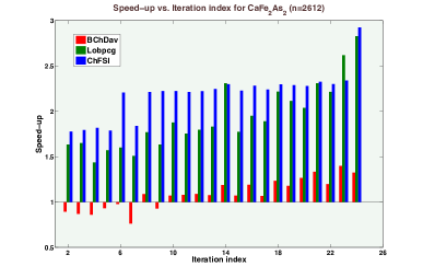
(a) Speed-up

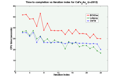
(b) Time to completion

Figure 2: Comparison between the 3 most effective block iterative eigensolvers for CaFe₂As₂ with respect to the outer-iteration index.

Lobpcg – Quite different is the performance of Lobpcg: this solver has speed-ups larger than 1.5X already at the beginning of the sequence. Both figures show that as the sequence progresses, Lobpcg speed-up presents moderate oscillations instead of a steady increase. Moreover while it reaches more than 2.5X for the last two outer-iteration indices of the CaFe₂As₂ system, it never does so for the larger system. The oscillation could be the consequence of different eigenvalue clustering for eigenproblems of distinct iteration indices. The decrease in speed-up for the larger system can be explained by the effectiveness of the conjugate gradient method to converge vectors even when Lobpcg is inputted random vectors. Conversely this trend implies a decreasing threshold for the speed-up for larger matrix sizes as signaled by the flattening of the CPU time curve in going from Figure 2 to Figure 3. This last observation suggests that, despite the nice speed-up, Lobpcg may take less and less advantage of approximate solutions as the size of the eigenproblem increases.

ChFSI – Among all the eigensolvers ChFSI seems to be able to take greater advantage of the approximate solutions and have a more predictable behavior: in plot (a) of Figure 2 its speed-up proceeds in 3 different steps jumping from $\sim 1.8$X to $\sim 2.2$X and to almost 3X at the end of the sequence. In Figure 3 the same trend appears in just two steps: ChFSI speed-up starts at $\sim 2$X and reaches just above 3X towards the end of the sequence. In the next subsection we explain in more detail the reasons for this step-like behavior. For the moment it is enough to say that ChFSI exploitation of approximate solutions seems to increase with the matrix size. This aspect together with the fact that its CPU time curve is not very different from Lobpcg’s delivers a better promise for this eigensolver to be the optimal one to take advantage of the correlation magnification as the sequence progresses. With this last consideration in mind we decided to single out ChFSI and implement it in the more efficient C programming language in order to be able to evaluate its performance and scalability.

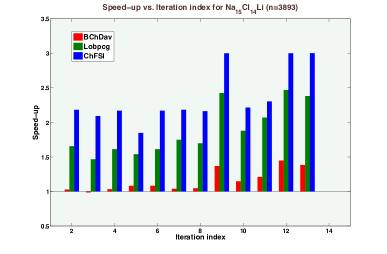
(a) Speed-up

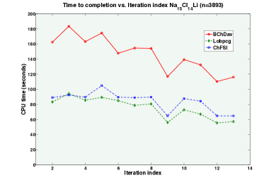
(b) Time to completion

Figure 3: Comparison between the 3 most effective block iterative eigensolvers for Na₁₅Cl₁₄Li with respect to the outer-iteration index.

We conclude this small section reiterating that, despite the differences in their behavior, all eigensolvers considered succeed to exploit the eigenvectors increasing collinearity, confirming the expectations that motivated this study.

3.3.2 The performance of ChFSI

The numerical tests of this section have their origin in an C language implementation of ChFSI that, for sake of clarity, we will refer to as ChFSIc. Besides being able to carry out performance tests, this implementation also allows us to run ChFSIc on JUROPA, a Jülich-based general purpose cluster with a large memory per node (24 Gb). We are able now to run the same tests of Section 3.3.1 on the larger matrix size systems of Table 1. The immediate objective is to verify the claim we made over the proportionality between eigenproblem size and effectivity of the algorithm to exploit approximate solutions.

Figure 4 clearly shows a tendency for the speed-up to grow as the size of the matrices increases. A closer analysis suggests that the extent of the speed-up is not only influenced by the iteration index, but additionally by the sought-after eigenspectrum fraction. From both plots it seems that both factors play a not-easy-to-predict role in the trend towards higher effectivity. A closer look at the algorithm (see Algorithm 1) reveals that speed-up is strongly related to the number of inner-loops that are necessary for all the eigenpairs to converge. Experimentally we observed that the total number of loops required by any eigenproblem is well below 10 and tends to decrease suddenly by one or more units every few outer-iteration cycles. For larger eigenproblem sizes this transition typically happens at later outer-iteration indices. For instance in plot (a) of Figure  4 the number of inner loops goes from 4 to 3 at the ninth iteration for $n=6217$, while the same change happens at the twelfth iteration for $n=9273$.

Table 4: Number of inner loop and filtered vectors w.r.t. iteration index for $n=8970$

Iteration Index	11	12	13	$\dots$	17	18	19	20	21
Number of loops	6	6	5	$\dots$	5	4	5	4	4
Number of filtered vectors	2794	2366	1999	$\dots$	1839	1766	1807	1711	1680

In the same figure plot (b) follows the same trend of plot (a) with the difference that the speed-up amplification is more gradual than step-like. Consider for example the $n=8970$ case, and observe the increase in speed-up from iteration index 10 on with the help of the data printed in Table 4. We can notice that there are two jumps in the number of loops: a sharp one between indices 12 and 13 where the total number of filtered vectors decreases suddenly by a factor of more than 200, and a less definite one across the range of indices 17-20. In the latter the total number of filtered vectors does not change so dramatically. In practice progressively less vectors are filtered during the fifth loop and progressively more by the fourth loop. There is not a sharp transition here probably due to the absence of a large block of vectors that suddenly succeed to converge during the fourth loop. This behavior of the algorithm does not make it less effective but indicates that eigenproblems appearing in materials without an energy gap can affect the behavior of the filter.

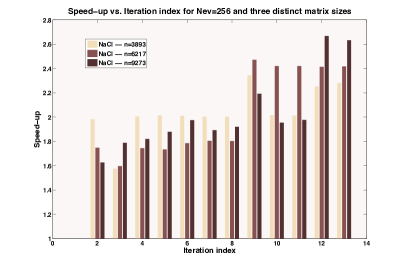
(a) Speed-up for Na₁₅Cl₁₄Li.

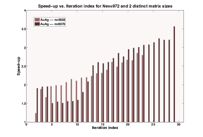
(b) Speed-up for Au₉₈Ag₁₀.

Figure 4: Speed-up for distinct matrix sizes. The matrix sizes are determined by distinct choices for K_max: namely K_max = $[3.0\ 3.5\ 4.0]$ for Na₁₅Cl₁₄Li, and K_max = $[3.0\ 3.5]$ for Au₉₈Ag₁₀. The speed-up is plotted with respect to the outer-iteration index.

Since realistic utilization of an iterative eigensolver in a FLAPW-based code requires evidence of scalability when used on multiple cores, we proceeded to test ChFSIc in a final set of numerical tests. From the pie chart in Figure 5 one can observe that the great majority of computational time for the sequential code is spent on the Chebyshev filter fraction (see Algorithm 1). The data refers to the algorithm as used with approximate solutions and the fractions of computational time remain pretty much the same for any system tested. In turn this chart suggests that parallelizing the filter is the first priority in order to scale on many cores. Since the Chebyshev filter uses almost entirely BLAS-3 kernels, it seems natural to call a multi-threaded version of BLAS.

For our tests we used MKL BLAS version 11.0 (Intel compiler version 12.0.3) over the possible range of cores available on one node of JUROPA. In plot (b) of Figure 5 speed-up of total execution of ChFSIc w.r.t. the number of cores is illustrated for three larger increasingly eigenproblems. As expected, the larger the physical systems the better it scales over an increasing number of cores. What is remarkable is the efficiency of the algorithm: due to the repetitive use of the ZGEMM routine by the polynomial filter, its scalability is as close to ideal as one can hope for. Clearly we do not claim this is the whole story, but it is suggestive of what ChFSIc could deliver when opportunely parallelized for a larger number of cores. Ultimately such a parallelization would allow the community of computational materials scientists to simulate larger and larger systems: an objective that is difficult to achieve with the present implementations of FLAPW-based codes.

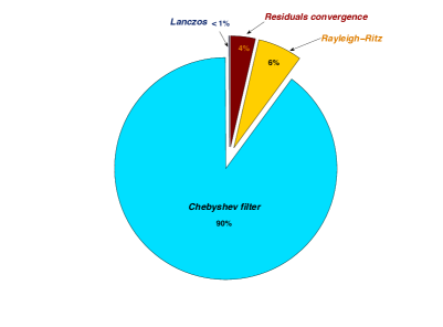
(a) CPU time for sequential fractions of the algorithm. The fractions refer to computation on the n=8970 system.

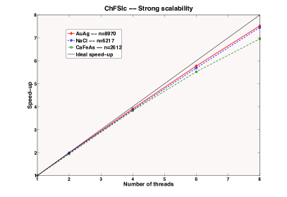
(b) Strong scalability on one computing node using multi-threaded BLAS.

Figure 5: The ChFSIc promise for optimal scalability. All measurements refer to the use of the algorithm when inputted approximate solutions.

4 Summary and conclusions

Sequences of generalized eigenvalue problems emerge in many common applications. In DFT they arise quite naturally in the search for a self-consistent solution for a set of coupled non-linear eigenvalue equations. In the FLAPW method, the matrix pencils making up each sequence are dense and are generally solved in isolation using direct solvers straight out of standard libraries. In this paper we started off from the idea that a sequence of eigenproblems should be considered as a whole and solved accordingly. The final aim is to uncover the possibility of a different approach where the connecting factor between eigenproblems can be exploited to accelerate the solution of the entire sequence.

To this end we illustrate the existence of the correlation between eigenpencils: subspace angles between eigenvectors of adjacent problems decrease monotonically as the sequence progresses towards convergence of the FLAPW DFT self-consistent cycle. In other words, eigenproblems of growing outer-iteration indices enjoy increasingly collinear eigenvectors. Our approach focuses on exploiting this property of the sequence by employing an iterative eigensolver tailored to accept the solution of an eigenproblem at a certain iteration to solve the eigenproblem at the next one. Out of the several variants of currently available iterative methods we selected three promising eigensolvers and proceeded to devise numerical experiments to test the alternative approach. In the context of the FLAPW method this is a novel and unexplored methodology.

The block solvers we evaluate represent three different classes of iterative methods: Davidson, conjugate gradient and subspace iteration methods. We carried out an exhaustive series of CPU time measurements for each algorithm. Times to reach solution were taken initializing the solvers with both random vectors and approximate solutions with respect to the outer-iteration index. Each measurement was performed for eigenproblems of different sizes, a 5-10% range of sought-after eigenspectrum, and sequences $\{P^{(\ell)}\}$ of increasing length. Speed-ups were plotted as the ratio between “random” over “approximate” CPU times.

The numerical results show that all eigensolvers take an increasing advantage of the approximate solutions as the outer-iteration index increases. While BChDav is probably over penalized by its use on dense eigenproblems, Lobpcg and ChFSI seem to be able to counter-balance their non-optimal use by substantially increasing their performance. In particular both solvers experience a speed-up larger than 2.5X towards the end of the sequence. These results carry evidence that a different approach to solve sequences of correlated eigenproblems arising in DFT is not only possible but desirable.

Among the three solvers ChFSI seems to have an extra performance edge thanks to a consistent increase of effectivity for larger sized systems. This result is confirmed by numerical tests run on a C language version of the algorithm and it is further strengthened by the promise for excellent scalability of this eigensolver: when the solver is run in a multi-threaded BLAS environment it scales increasingly better for larger sized eigenproblems reaching an efficiency above 85%. Since the size of the eigenproblems depends linearly on the number of atoms, optimal scalability is the crucial element which enables the use of a larger number of processors in order to maximally expand the size of the physical system that can be simulated [16].

In conclusion we observe that out of three iterative block eigensolvers, two of them greatly benefit from the use of approximated solutions. This result indicates the possibility of a different strategy in solving sequences of dense eigenproblems in the context of DFT. Instead of using a direct solver for each single eigenproblem in isolation it could be more efficient to exploit the numerical properties of the sequence as a whole. Eventually this change in strategy could lead to substantial speed-up of the entire self-consistent outer-iterative process.

While our conclusions constitute a proof of concept, they do not claim to be an exhaustive performance analysis. Some of the described algorithms are already available on working platforms more appropriate for performance studies [17]. Moreover, current efforts are underway to parallelize ChFSIc for shared, distributed and hybrid architectures and a thorough study on its performance will be presented in a follow-up publication. Eventually, our goal is to conclusively demonstrate that, despite the dense nature of DFT eigenproblems, a promising block iterative eigensolver like ChFSIc together with an appropriate strategy to reuse previous solutions, can be competitive with direct solvers when only a fraction of the eigenspectrum is sought after.

The authors would like to thank Prof. Bientinesi for his support, collaboration and steady flow of suggestions, Dr. Wortmann for his prompt support with the use of FLEUR and the provision of the physical systems for the numerical tests, Prof. Zhou for kindly providing one of the Matlab routines used in running the numerical tests, Prof. Stathopoulos for his suggestions and finally Prof. Blügel for his enthusiasm and support for our ideas. A special acknowledgement to the Jülich Supercomputing Centre and the John von Neumann Institute for Computing for providing the computational resources to perform all numerical experiments.

References

- [1] R. M. Dreizler, and E. K. U. Gross, Density Functional Theory (Springer-Verlag, 1990)
- [2] W. Kohn, and L. J. Sham, Phys. Rev. A 140 (1965) 1133
- [3] P. Hohenberg and W. Kohn, Phys. Rev. B 136 (1964) 864
- [4] A. J. Freeman, H. Krakauer, M. Weinert, and E. Wimmer, Phys. Rev. B 24 (1981) 864.
- [5] A. J. Freeman, and H. J. F. Jansen, Phys. Rev. B 30 (1984) 561
- [6] M. Benzi, P. Boito, and N. Razouk, SIAM Rev., vol. 55 (2013) 3-64, [arXiv:1203.3953v1]
- [7] E. Di Napoli, S. Blügel, and P. Bientinesi, Comp. Phys. Comm. 183 (2012), pp. 1674-1682, [arXiv:1108.2594]
- [8] G. W. Stewart, SIAM J. Matrix Anal. Appl. 23 (2002) 601
- [9] Y. Saad, Numerical methods for large eigenvalue problems (SIAM, 2011)
- [10] Y. Zhou, and Y. Saad, Numer. Algor. 47 (2008) 341
- [11] Y. Zhou, and Y. Saad, SIAM J. Matrix Anal. Appl. 29 (2007) 954
- [12] Y. Zhou, J. Comp. Phys. 229 (2010) 9188
- [13] A. Knyazev, SIAM J. Sci. Comput. 23 (2001) 517
- [14] Y. Zhou, Y. Saad, M. L. Tiago, J. R. Chelikowsky, J. Comp. Phys. 219 (2006) 172
- [15] Y. Zhou, Y. Saad, M. L. Tiago, J. R. Chelikowsky, Phys. Rev. E 74 (2006) 066704
- [16] L. Snyder, Annu. Rev. Comput. Sci. vol. 1 (1986) 289
- [17] A. Stathopoulos and J. R. McCombs, ACM Trans. Math. Soft. 37 (2010) 21:1
- [18] S. Blügel, G. Bihlmayer, D. Wortmann, C. Friedrich, M. Heide, M. Lezaic, F. Freimuth, and M. Betzinger, The Jülich FLEUR project - http://www.flapw.de
- [19] P. Blaha, K. Schwarz, G. Madsen, D. Kvasnicka and J. Luitz, WIEN2k - http://www.wien2k.at/
- [20] M. Weinert, R. Podloucky, J. Redinger and G. Schneider, FLAIR - https://pantherfile.uwm.edu/weinert/www/flair.html
- [21] C. Ambrosch-Draxl, Z. Basirat, T. Dengg, R. Golesorkhtabar, C. Meisenbichler, D. Nabok, W. Olovsson, P. asquale Pavone, S.Sagmeister, and J. Spitaler, The Exciting Code - http://exciting-code.org/
- [22] J. K. Dewhurst, S. Sharma, L. Nordström, F. Cricchio, F. Bultmark, and E. K. U. Gross, The Elk Code Manual (Ver. 1.2.20) - http://elk.sourceforge.net/
- [23] E. Anderson, Z. Bai, C. Bischof, L.S. Blackford, J. Demmel, Jack J. Dongarra, J. Du Croz, S. Hammarling, A. Greenbaum, A. McKenney, and D. Sorensen, LAPACK Users’ guide, (Society for Industrial and Applied Mathematics, Philadelphia, PA USA, (third ed.), 1999)
- [24] L.S. Blackford, J. Choi, A. Cleary, E. D’Azeuedo, J. Demmel, I. Dhillon, S. Hammarling, G. Henry, A. Petitet, K. Stanley, D. Walker, and R.C. Whaley, ScaLAPACK user’s guide, (Society for Industrial and Applied Mathematics, Philadelphia, PA USA, 1997)
- [25] D.D. Johnson, Phys. Rev. B 38, (1988) 12807.
- [26] S. Blügel Forschungszentrum Jülich, Report 2197, 1988.
- [27] J. R. Chelikowsky The PARSEC code http://parsec.ices.utexas.edu/