Self-avoiding walks on a bilayer Bethe lattice

Abstract

We propose and study a model of polymer chains in a bilayer. Each chain is confined in one of the layers and polymer bonds on first neighbor edges in different layers interact. We also define and comment results for a model with interactions between monomers on first neighbor sites of different layers. The thermodynamic properties of the model are studied in the grand-canonical formalism and both layers are considered to be Cayley trees. In the core region of the trees, which we may call a bilayer Bethe lattice, we find a very rich phase diagram in the parameter space defined by the two activities of monomers and the Boltzmann factor associated to the interlayer interaction between bonds or monomers. Beside critical and coexistence surfaces, there are tricritical, bicritical and critical endpoint lines, as well as higher order multicritical points.

I Introduction

The theoretical study of the thermodynamic behavior of polymers, both in a melt or in solution, has a long history, continuous and lattice models were proposed to study such systems f66 . In lattice models, the first approach is to consider the linear polymeric chains to be random walks, this model is sometimes called ideal chain approximation. A more realistic approach is to represent the linear polymeric chains by self- and mutually avoiding walks (SAW’s), and therefore one of the simplest models is athermal, since only the excluded volume interactions are taken into account. Regarding the phase transitions which happen in such models, the excluded volume interactions are essential, at space dimensions below the upper critical dimension, to produce the correct critical exponents dg79 . At and above the upper critical dimension the ideal chain exponents are found. In a grand-canonical ensemble, at low activities of monomers, a non-polymerized phase is stable, but as the activity is increased, a transition to a polymerized phase happens. This transition is usually continuous.

While a simple model with excluded volume interactions may explain the polymerization transition when the chains are placed in a good solvent, in bad solvents and at low temperatures collapsed configurations are favored energetically. Below the temperature ($\Theta$ point), at which the transition between the extended and the collapsed configurations happens, the polymerization transition is discontinuous, so that the collapse transition corresponds to a tricritical point. This transition is frequently named coil-globule transition in the literature. A simple effective model which explains this phenomena includes attractive interactions between monomers placed at first neighbor sites which are not consecutive along a chain, these interactions favor more compact polymer configurations, thus reducing the contact area of the polymer chain with the solvent. In the literature, these interacting walks are called self-attractive self-avoiding walks (SASAW’s) dg79 . When it was realized by De Gennes that the simple polymerization model could be mapped on the ferromagnetic $n$-vector model in the limit when the number of components of the order parameter $n$ vanishes dg72 , the then new ideas of renormalization group, in the form of and expansion of critical exponents in $\epsilon=4-d$ with coefficients which are functions of $n$, where $d$ is the spacial dimensionality of the system, could be directly applied to models for polymers. A detailed discussion of this limit may be found in wp81 . Later, the relation between polymers and magnetic models was extended to SASAW’s dg75 . Related to this problem of the collapse transition of a polymer chain with effective attractive interactions, a related problem of two chemically distinct chains with attractive interactions between them has also been studied in the literature. As in the case of SASAW’s, the phase diagrams of such systems also display a tricritical point, the collapsed state corresponds in this case to a zipped state, where steps for which the bonds of both chains move side by side are favored. The solution of this model on fractal lattices such as the $2D$ Sierpinski gasket ks93 and truncated $n$-simplex lattice ks95 , where real space renormalization transformations are exact, leads to phase diagrams with tricritical points also, as is the case for SASAW’s.

Although it is rather natural to consider the effective attractive interactions in the SASAW’s to be between monomers, as described above, in the literature an alternative model, with interactions between bonds in the same elementary polygon of the lattice (plaquette) has also received much attention, one of the reasons for this is that this model may be mapped on the $n$-vector model with four spin interactions bn89 ; wp81b . One may imagine that the two SASAW’s models, with interactions between monomers or bonds, should lead to similar thermodynamic properties, but at least on two-dimensional lattices this is not the case. Qualitatively different phase diagrams were found for both models on a four coordinated Husimi lattice sms96 and in transfer matrix calculations combined with FSS extrapolations on the square lattice mos01 .

The behavior of magnetic models on bilayers and multilayers has attracted attention in the literature for quite some time. For example, coupling through non magnetic layers shows oscillatory behavior and may lead to giant magnetoresistance effects b88 . The phase diagrams of magnetically disordered bilayers have been studied on a system of two adjacent coupled Bethe lattices, for competing intralayer interaction parameters, the phase diagram displays multiple reentrant behavior ld92 . A variety of other magnetic systems has also been studied on similar lattices albayrak . Although, as expected, Bethe lattice solutions overestimate the region of stability of ordered phases, they may furnish the general features of phase diagrams.

Polymeric chains close to interfaces between two immiscible liquids have also been studied, and it was found in a continuum model that the chains are attracted to the interface hp86 , the maximum of the distribution of monomers being located close to the interface, inside the better solvent. A similar model was also studied in w86 , with a different parametrization and several mean values and probabilities related to the conformation of the polymer chain are evaluated. The behavior of a copolymer close to a bilayer has been considered also in the literature, motivated by the relation of this problem with the relevant biological problem of the localization of a protein in a lipid bilayer ermoshkin02 . Two regimes are found in this study regarding the localization of the chain in the bilayer. In the first, the density of monomers is a bimodal function, with maxima centered on the two interfaces, while the second configuration displays a single maximum of the density in the center of the bilayer. In the bimodal regime, few monomers are present in the area between the interfaces and most of the chain is adsorbed on them.

Here we address a simpler problem, with homopolymer chains only, in the limit where each chain is entirely adsorbed on one layer and thus no polymer bond is present linking chains adsorbed on different interfaces. We include in the model interactions between polymer bonds placed in different layers on corresponding edges. This interaction takes into account the changes in statistical weight of a polymer bond if it is in contact with the other solvent across the interface or with a bond of another polymeric chain in the other interface. In figure 1 a particular configuration of a part of a bilayer built with two square lattices is shown. Although we show in details the calculations and results of the model with interacting bonds, we have also studied the alternative model where the interactions are between monomers, and will briefly discuss the differences in the thermodynamic behaviors of the models. In what follows, we consider both interfaces to be Cayley trees of arbitrary coordination number $q$, with polymeric chains on them whose endpoints are placed on the surface sites of the trees. Since we will study the behavior of the model in the core of the bilayer tree, we may consider this solution of the model to be a Bethe approximation for the model on regular lattices with the same coordination number.

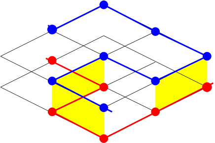
Figure 1: (color online) Part of a bilayer square lattice with a polymer chain on each layer. The three pairs of interacting bonds are edges of the shadowed (yellow) rectangles. In the model with interactions between monomers, five pairs of interacting monomers are present in the figure.

The paper is organized as follows: In section II we define the model more precisely on the bilayer Bethe lattice and obtain its solution in terms of fixed points of recursion relations. The fixed points which are stable in some region of the parameter space are presented in section III, studying the stability of these fixed points we address the transitions between the phases which are associated to each physical fixed point. The phase diagram in the three-dimensional parameter space of the model is studied in some detail in section IV, and final discussions and conclusion may be found in section V

II Definition of the model and solution on the bilayer Bethe lattice

The problem is defined in the grand-canonical formalism, so that the parameters of the model are the fugacities of a polymer bond in layer 1, $x_{1}=\exp[\mu_{1}/(k_{B}T)]$, and in layer 2, $x_{2}=\exp[\mu_{2}/(k_{B}T)]$, as well as a Boltzmann factor $\chi=\exp[\epsilon/(k_{B}T)]$ for each pair of polymer bonds of corresponding edges or corresponding monomers in different layers. The energy of interaction of these pairs of bonds or monomers is, therefore, equal to $-\epsilon$, and is attractive if $\epsilon>0$. In what follows, we restrict ourselves to the model of interacting bonds, unless otherwise stated. In figure 2 a particular configuration of the model is shown for a bilayer Bethe lattice with coordination number equal to three.

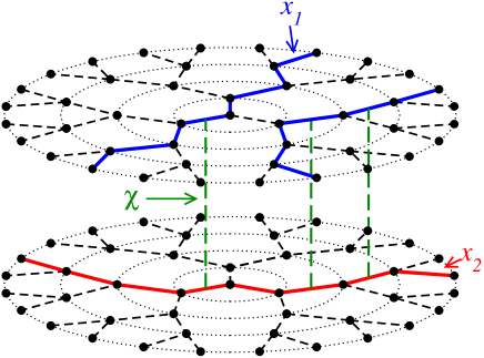
Figure 2: (color online) Bilayer Bethe lattice with $q=3$ and $M=4$ generations. The polymer configuration has a statistical weight $x_{1}^{14}\,x_{2}^{8}\,\chi^{3}\,=\,x_{1}^{11}\,x_{2}^{5}\,\kappa^{3}$, where $\kappa=x_{1}x_{2}\chi$.

The grand-canonical partition function of the model may be written as

$${\cal Y}\,=\,\sum\;x_{1}^{N_{1}}\;x_{2}^{N_{2}}\;\chi^{N_{B}}$$ (1)

where the sum is over configurations of self and mutually avoiding walks placed on the trees. The endpoint monomers of the walks are placed on the surface sites of the trees. $N_{1}$ is the number of polymeric bonds on the Cayley tree 1, $N_{2}$ is the number of polymeric bonds on the Cayley tree 2, and $N_{B}$ is the number of pairs of polymeric bonds located on first neighbor edges on different trees. We refer to figure 2 for the statistical weight of a particular configuration of the system.

The solution of systems defined on tree-like structures defining recursive relations for partial partition functions (ppf’s) is well known baxter , and is particularly useful for polymeric models because it is simple to impose the excluded-volume condition ss90 ; ss07 . The generalization to a bilayer Bethe lattice is straightforward, and was widely used to study magnetic bilayers ld92 ; albayrak . We thus proceed defining partial partition functions for rooted sub-trees. The fixed root configuration of these sub-trees is specified by the polymer bonds which arrive at the root sites of sub-trees 1 and 2 coming from outer generations of sites. We need four partial partition functions: $g_{0,0},\;g_{1,0},\;g_{0,1},$ and $g_{1,1}$ where the first (second) sub-index denotes the numbers of polymers bonds incident at the root site of the sub-tree 1 (2). Considering the operation of attaching $q-1$ sub-trees to a new pair of root sites, we may write recursion relations for the partial partition functions of a sub-tree with one additional generation of sites, denoted by primes. The recursion relations are:

$$g^{\prime}_{0,0} = g_{0,0}^{q-1}\,+\,\frac{1}{2}(q-1)(q-2)\left(x_{1}^{2}\,g_{1,0}^{2}\,+\,x_{2}^{2}\,g_{0,1}^{2}\right)\,g_{0,0}^{q-3}\,+\,$$ (2a)

$$(q-1)(q-2)(q-3)\,x_{1}^{2}\,x_{2}^{2}\,\chi\,g_{1,1}\,g_{1,0}\,g_{0,1}\,g_{0,0}^{q-4}\,+\,$$

$$\frac{1}{2}(q-1)(q-2)\,x_{1}^{2}\,x_{2}^{2}\,\chi^{2}\,g_{1,1}^{2}\,g_{0,0}^{q-3}\,+\,$$

$$\frac{1}{4}(q-1)(q-2)(q-3)(q-4)\,x_{1}^{2}\,x_{2}^{2}\,g_{1,0}^{2}\,g_{0,1}^{2}\,g_{0,0}^{q-5}\,,$$

$$g^{\prime}_{1,0}\, = \,(q-1)\,x_{1}\,g_{1,0}\,g_{0,0}^{q-2}\,+\,(q-1)(q-2)\,x_{1}\,x_{2}^{2}\,\chi\,g_{1,1}\,g_{0.1}\,g_{0,0}^{q-3}\,+\,$$ (2b)

$$\frac{1}{2}(q-1)(q-2)(q-3)\,x_{1}\,x_{2}^{2}\,g_{1,0}\,g_{0,1}^{2}\,g_{0,0}^{q-4}\,,$$

$$g^{\prime}_{0,1}\, = \,(q-1)\,x_{2}\,g_{0,1}\,g_{0,0}^{q-2}\,+\,(q-1)(q-2)\,x_{1}^{2}\,x_{2}\,\chi\,g_{1,1}\,g_{1,0}\,g_{0,0}^{q-3}\,+\,$$ (2c)

$$\frac{1}{2}(q-1)(q-2)(q-3)\,x_{1}^{2}\,x_{2}\,g_{1,0}^{2}\,g_{0,1}\,g_{0,0}^{q-4}\,,$$

$$g^{\prime}_{1,1}\, = \,(q-1)\,x_{1}\,x_{2}\,\chi\,g_{1,1}\,g_{0,0}^{q-2}\,+\,(q-1)(q-2)\,x_{1}\,x_{2}\,g_{1,0}\,g_{0,1}\,g_{0,0}^{q-3}\,.$$ (2d)

The ppf’s grow exponentially with the iterations, so, as usual, it is convenient to define ratios of the ppf’s, and the thermodynamic properties of the model may be expressed by the fixed point values of these ratios. The ratios we use are:

$$R_{1}=x_{1}\,\frac{g_{1,0}}{g_{0,0}}\;,\;\;R_{2}=x_{2}\,\frac{g_{0,1}}{g_{0,0}}\;,\;\;R_{3}=x_{1}\,x_{2}\,\chi\,\frac{g_{1,1}}{g_{0,0}}\;.$$ (3)

The recursion relations for the ratios will be

$$R^{\prime}_{1}\, = \,\left[(q-1)R_{1}\,+\,(q-1)(q-2)\,R_{2}R_{3}\,+\,\frac{1}{2}(q-1)(q-2)(q-3)\,R_{1}R_{2}^{2}\,\right]\frac{x_{1}}{D}\,,$$ (4a)

$$R^{\prime}_{2}\, = \,\left[(q-1)R_{2}\,+\,(q-1)(q-2)R_{1}R_{3}\,+\,\frac{1}{2}(q-1)(q-2)(q-3)\,R_{1}^{2}R_{2}\,\right]\frac{x_{2}}{D}\,,$$ (4b)

$$R^{\prime}_{3}\, = \,\left[(q-1)R_{3}\,+\,(q-1)(q-2)\,R_{1}R_{2}\,\right]\frac{\kappa}{D}\,,$$ (4c)

where $\kappa\equiv x_{1}\,x_{2}\,\chi$, and

$$D = 1+\frac{1}{2}(q-1)(q-2)\left(R_{1}^{2}+R_{2}^{2}+R_{3}^{2}\right)+(q-1)(q-2)(q-3)\,R_{1}R_{2}R_{3}\,+$$ (5)

$$\frac{1}{4}(q-1)(q-2)(q-3)(q-4)R_{1}^{2}R_{2}^{2}.$$

Connecting $q$ sub-trees to the central site of the Cayley tree, the grand-canonical partition function takes the form

$$\frac{{\cal Y}}{g_{00}^{q}}\,\equiv\,Y = 1+\frac{1}{2}q(q-1)\left(R_{1}^{2}+R_{2}^{2}+R_{3}^{2}\right)\,+\,q(q-1)(q-2)\,R_{1}R_{2}R_{3}\,+\,$$ (6)

$$\frac{1}{4}q(q-1)(q-2)(q-3)R_{1}^{2}R_{2}^{2}\,.$$

The Bethe lattice solution of the model corresponds to its behavior in the core of the Cayley tree, so that surface effects are eliminated. The corresponding dimensionless free energy per site may be found using a prescription proposed by Gujrati g95 . The result is

$$\phi_{b}\,=\,-\frac{1}{2}\left[q\ln{(D)}\,-\,(q-2)\ln{(Y)}\right].$$ (7)

This expression may be derived quite easily supposing that the free energy of the model on the whole Cayley tree (divided by $k_{B}T$) may be written as $\Phi=-\ln{\cal Y}=N_{s}\phi_{s}+N_{b}\phi_{b}$, where $\phi_{s}$ and $\phi_{b}$ are the free energies per site for the $N_{s}$ surface and $N_{b}$ bulk sites, respectively. Considering the free energies of the model on two Cayley trees with $M$ and $M+1$ generations in the thermodynamic limit $M\to\infty$ one may then obtain an expression for the bulk free energy per site $\phi_{b}$. A slightly more general argument which leads to the same result may be found in oss09

III physical fixed points

The phase diagram is obtained looking for the physical fixed points of the recurrence relations Eqs.(4). For physical fixed point we understand that there exists a region in the thermodynamic space $(x_{1},x_{2},\kappa)$ where the fixed point is stable and corresponds to a global minimum of the free energy Eq.(7), thus representing a thermodynamic phase. A fixed point $R^{*}\,=\,(R_{1}^{*},R_{2}^{*},R_{3}^{*})$ is stable if the Jacobian matrix

$${\cal J}_{i,j}\,=\,\left.\frac{\partial R^{\prime}_{i}}{\partial R_{j}}\right|_{R^{*}}$$ (8)

has all the eigenvalues less than one. We found five stable fixed points describing five different thermodynamic phases:

III.0.1 Nonpolymerized fixed point ($NP$)

The $NP$ fixed point is given by $R_{1}^{(NP)}=0;\,R_{2}^{(NP)}=0;\,R_{3}^{(NP)}=0$, which corresponds to a phase where the density of polymers vanished in both trees. The Jacobian matrix is

$${\cal J}^{(NP)}\,=\,\left(\begin{array}[]{cccc}(q-1)\,x_{1}&0&0\\ \\ 0&(q-1)\,x_{2}&0\\ \\ 0&0&(q-1)\,\kappa\end{array}\right)\;,$$ (9)

thus the stability limits for the $NP$ phase are given by the conditions

$$x_{1}^{(NP)}\,=\,\frac{1}{q-1}\;,\;\;x_{2}^{(NP)}\,=\,\frac{1}{q-1}\;,\;\;\kappa^{(NP)}\,=\,\frac{1}{q-1}\;.$$ (10)

III.0.2 Fixed point with polymers on the tree 1 ($P_{1}$)

The fixed point $R_{1}\neq 0;\,R_{2}=0;\,R_{3}=0$, corresponds to a phase where the density of polymers is nonzero on the Bethe lattice numbered as one, and zero on the other lattice. The fixed point point value of the ratio $R_{1}$ is $R_{1}^{(P_{1})}=\sqrt{2[(q-1)x_{1}-1]/[(q-1)(q-2)]}$, and therefore we may obtain the elements of the Jacobian matrix in terms of the parameters of the model. The result is

$${\cal J}^{(P_{1})}\,=\,\left(\begin{array}[]{cccc}\frac{2-(q-1)\,x_{1}}{(q-1)\,x_{1}}&0&0\\ \\ 0&\frac{[2+(q-1)(q-3)x_{1}]x_{2}}{(q-1)\,x_{1}}&\sqrt{\frac{2(q-2)\,[(q-1)x_{1}-1]}{q-1}}\;\frac{x_{2}}{x_{1}}\\ \\ 0&\sqrt{\frac{2(q-2)\,[(q-1)x_{1}-1]}{q-1}}\frac{\kappa}{x_{1}}&\frac{\kappa}{x_{1}}\end{array}\right)\;.$$ (11)

For this phase, the stability limits are given by

$$x_{1}^{(P_{1})}\,=\,\frac{1}{q-1}\;,\;\;\ \kappa\,=\,x_{1}\frac{2x_{2}+(q-1)x_{1}[(q-3)x_{2}-1]}{(q-1)[2x_{2}-(q-1)x_{1}x_{2}-x_{1}]}\;.$$ (12)

III.0.3 Fixed point with polymers on the tree 2 ($P_{2}$)

The fixed point $R_{1}=0;\,R_{2}\neq 0;\,R_{3}=0$ corresponds to a phase where the density of polymers is nonzero in the Bethe lattice numbered as two, and vanishing on the other lattice. By symmetry, the stability limits of the $P_{2}$ fixed point may be obtained from the stability limits of the $P_{1}$ fixed point Eq. (12) interchanging $x_{1}$ and $x_{2}$.

III.0.4 Polymerized fixed point ($P$)

For this fixed point $R_{1}\neq 0;\,R_{2}\neq 0;\,R_{3}\neq 0$, so that the density of polymers is nonzero on both trees. In this case the stability lines were calculated numerically.

III.0.5 Bilayer fixed point ($P_{B}$)

This fixed point $R_{1}=0;\,R_{2}=0;\,R_{3}\neq 0$ corresponds to a phase where all polymer bonds are placed in pairs on corresponding edges of both trees, so that the polymer of both layers are fully correlated. The Jacobian matrix of this fixed point is

$${\cal J}^{(P_{B})}\,=\,\left(\begin{array}[]{cccc}\frac{x_{1}}{\kappa}&\sqrt{\frac{2(q-2)((q-1)\kappa-1)}{q-1}}\,\frac{x_{1}}{\kappa}&0\\ \\ \sqrt{\frac{2(q-2)((q-1)\kappa-1)}{q-1}}\,\frac{x_{2}}{\kappa}&\frac{x_{2}}{\kappa}&0\\ \\ 0&0&\frac{2-(q-1)\,\kappa}{(q-1)\,\kappa}\end{array}\right)\;,$$ (13)

and the stability limits are given by

$$x_{2}^{(P_{B})}\,=\,\frac{(q-1)(\kappa-x_{1})\kappa}{(q-1)(1+2(q-2)x_{1})\kappa-(3q-5)x_{1}}\;,\;\;\kappa^{(P_{B})}\,=\,\frac{1}{(q-1)}\;.$$ (14)

IV phase diagram

The next step in order to obtain the phase diagram is to study the overlap between stability regions of different physical fixed points. If two regions where a unique fixed point is stable are separated by a common stability line, on this line a continuous phase transition is expected. If two or more fixed points are stable in the same region of the parameter space, this signals coexistence of phases. In this case, the loci of the discontinuous transitions may be found requiring that the coexisting phases should have the same (minimum) free energy. The five fixed points are present for coordination numbers $q\geq 3$, but for $q=3$ the equations are simpler and thus some of the calculations may be done analytically. Therefore, we performed all calculations below for $q=3$. Some changes in the phase diagrams may arise for $q>3$.

Since a rather large number of physical fixed points is found, the model has a rich phase diagram, with different multicritical lines. In figures 3-9 we show six $(x_{1},x_{2})$ cuts for $\kappa=0,\,1/4,\,1/3,\,9/20,\,1/2,\,1$. These values of $\kappa$ were chosen in order to illustrate the main features of the phase diagram. The second-order lines and multicritical points were obtained analytically, and the first-order lines were found numerically.

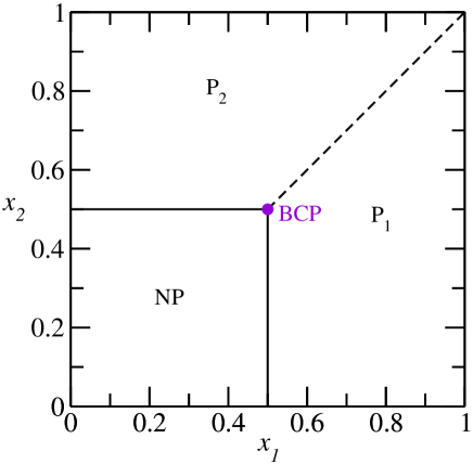
Figure 3: (Color online) Phase diagram for $\kappa=0$. The dashed (black) curve is a first order transition and the full (black) lines are continuous transitions between the $NP-P_{1}$ and $NP-P_{2}$ phases. The bicritical point BCP is represented by a (violet) dot. This and the following diagrams were all obtained for $q=3$.

The first diagram, for $\kappa=0$, is depicted in figure 3. It actually corresponds to infinite repulsive interactions between polymer bonds in corresponding edges of both lattices. Although it should be said that this limiting case is probably quite far away from real polymeric systems, the phase diagram exhibits interesting features which lead us to shortly discuss it here. If a polymerized phase exists in one of the lattices, its presence inhibits the polymerization transition on the other lattice, since it reduces the effective coordination number at this other lattice. This effect is apparent in the diagram, the transition to the phase $P_{2}$, at constant $x_{1}>1/(q-1)$ happens at $x_{2}=x_{1}>1/(q-1)$ and is discontinuous, since when the free energy of the $P_{1}$ phase becomes smaller than the one of the $P_{2}$ phase, $x_{1}$ is larger than its critical value $1/(q-1)$. The coexistence line of the two polymerized phases meets the two critical polymerization lines at a point which is a bicritical point (BCP), located at $x_{1}=x_{2}=1/(q-1)$. It is worth mentioning that the features of the transition lines incident at the BCP are the ones expected for a mean-field approximation as the one we are doing here: the classical crossover exponent is $\phi=1$, so that the critical lines are linear functions close to the BCP ba75 . In general, one finds $\phi>0$ and therefore the critical lines meet the coexistence line tangentially, as may be found, for instance, from $\epsilon=4-d$ expansions for the $n$-vector model when $n>0$ up to order $\epsilon^{4}$ k81 . However, all these coefficients vanish for $n\to 0$, so that it is possible that even below the upper critical dimension linear incidence of the critical lines at the BCP is observed.

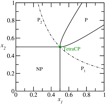
Figure 4: (Color online) Phase diagram for $\kappa=1/4$. The full (black) lines are continuous transitions. The green dot is a tetracritical point. In this and the following diagrams, on the dot-dashed (black) curve the interactions between the polymer bonds vanishes ($\chi=1$).

When $\kappa$ has a small positive value, the $P$ phase occupies a region between the $P_{1}$ and $P_{2}$ phases, separated from them by critical lines, as may be seen in figure 4. With this intermediate phase present, the bicritical point becomes a tetracritical point, similar to what is found in anisotropic antiferromagnets ba75 . Again the remarks about the crossover exponent $\phi$ and the incidence of the four critical lines at the tetracritical point apply, and for a mean-field approximation linear behavior is expected, in agreement with the results we obtained. In this and the following diagrams, the dot-dashed curve $x_{1}x_{2}=\kappa$ separates the regimes of repulsive ($\chi<1$) and attractive ($\chi>1$) interactions between the polymers; the tetracritical point is located on this curve. The region of attractive bond-bond interactions if situated below the curve. The two critical lines which limit the $P$ phase meet at a right angle. Between $\kappa=1/4$ and $\kappa=1/3$, this angle is larger than $\pi/2$, as may be seen in the phase diagram for $\kappa=1/3$ shown in figure 5, where the angle is equal to $\pi$. A point which may be worth discussing is that in this case a reentrant behavior is seen in the critical lines which limit the phase $P$. This behavior is actually a consequence of our choice of variables, since $\kappa=x_{1}x_{2}\chi=const.$ implies that the Boltzmann factor of the interactions $\chi$ is not constant if one of the activities changes. In a similar diagram with constant $\chi$ the critical curves are monotonous and no reentrance is seen.

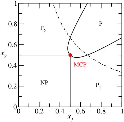
Figure 5: (Color online) Phase diagram for $\kappa=1/3$. All transitions are continuous. The point where the four critical lines meet is the endpoint of a line of tetracritical points for $\kappa<1/3$ and four other lines, two of them tricritical and two of critical endpoints, for $\kappa>1/3$, thus being a multicritical point of higher order. The dot-dashed curve corresponds to $\chi=1$.

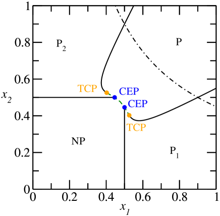
Figure 6: (Color online) Phase diagram for $\kappa=9/20$. Two pairs of tricritical points (orange) and critical endpoints (blue) appear.The dot-dashed curve corresponds to $\chi=1$.

As $\kappa$ exceeds $1/3$, a qualitative change of the phase diagram happens. The tetracritical point splits into two pairs of tricritical and critical endpoints, as may be seen in figure 6. A first order transition line now separates phase $P$ and $NP$, while part of the transition between phase $P$ and the phases $P_{1}$ and $P_{2}$ becomes discontinuous. As $\kappa$ grows, the tricritical points approach the $NP-P_{1}$ and the $NP-P_{2}$ critical lines and the critical endpoints, so that finally, at $\kappa=1/2$, the tricritical points meet the critical surface which limit the $NP$ phase, as may be seen in figure 7. The multicritical points where the tricritical and critical endpoint lines meet are labeled MCP1 in the diagram. The dotted line which connects the two multicritical points is a line of bicritical points, since at this line two critical surfaces ($NP-PB$ and $PB-P$) and a coexistence surface ($NP-P$) meet. At this value of $\kappa$, the critical lines between polymerized phases change from concave to convex, so that they are linear. The $NP$ phase is still stable in a region of the phase diagram close to the origin, but its stability is quadratic, so that the region covered by it in this phase diagram is actually a critical surface separating it from the bilayer polymerized phase $P_{B}$, which becomes stable for $\kappa>1/2$. On the lines between the multicritical points (MCP1 and MCP2), four critical surfaces meet ($NP-P_{2}$, $P_{2}-P$, $P-P_{B}$ and $P_{B}-NP$ on the upper part of the diagram), so that on this line we have tetracritical transitions. This feature may be better appreciated in the diagram in the variables $\kappa$ and $x_{2}$, for $x_{1}=1/3$, which cuts this line of tetracritical points and is shown in figure 8.

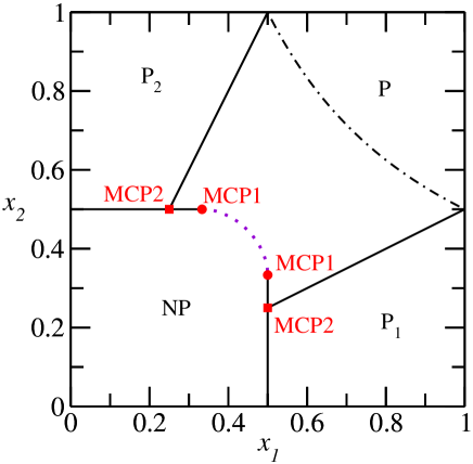
Figure 7: (Color online) Phase diagram for $\kappa=1/2$. The dotted (violet) curve is a line of bicritical points, and is limited by two multicritical points (red dots). Between these multicritical points and the multicritical points represented by squares, the critical lines $P_{2}-P$ and $P-NP$, as well as $P_{1}-P$ and $P-NP$ coalesce, so that on this line four critical surfaces meet, thus characterizing it as a tetracritical line (green).The dot-dashed curve corresponds to $\chi=1$.

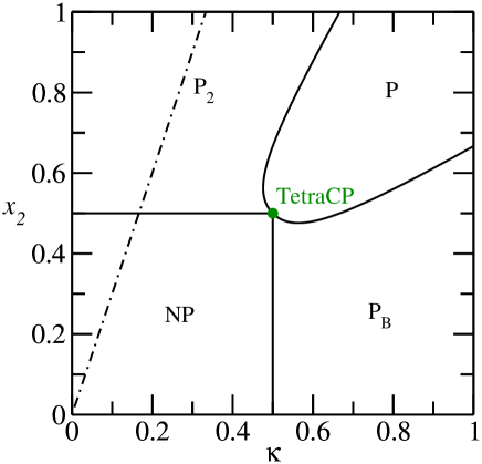
Figure 8: (Color online) Phase diagram in the variables $(\kappa,x_{2})$ for $x_{1}=1/3$. Four critical lines meet at a tetracritical point, represented by a circle (green).

As soon as $\kappa$ exceeds $1/2$ all transitions are continuous. The phase diagrams are similar to the one shown in figure 9, for $\kappa=1$. Graph (a) corresponds to the model with interacting bonds. All four polymerized phases are present, there are three critical lines separating the phase $P$ from another polymerized phase. Since the stability limits of the phases $P_{1}$, $P_{2}$, and $P_{B}$ are known (Eqs. (12) and (14)), the phase diagram may be obtained analytically. The critical lines which limit the phases $P_{1}$ and $P_{2}$ start at $x_{1}=0$ and $x_{2}=0$ respectively, thus $\kappa=1/2$ is a quite singular value regarding the behavior of these lines. As expected, the region of the parameter space where the $P_{B}$ phase is stable grows with increasing values of $\kappa$.

While figure 3 is the same for interactions between bonds or monomers, for nonzero values of $\kappa$ different phase diagrams are found for both models. As an example, in figure 9 we also show the result for the model with interaction between monomers (b). We have chosen to compare the thermodynamic properties of both models for larger values of $\kappa$ since obviously the differences between the results for both models are bigger. We notice that the bilayer polymerized phase is never the phase with lowest free energy for $\kappa=1$ if the interaction is between monomers, although this phase is the one with lowest free energy in the region of low values of $x_{1}$ and $x_{2}$, for $1/2<\kappa<1$. The larger region in the parameter space where the $P$ phase has lower free energy as the $P_{B}$ phase, when compared to the model with interacting bonds, may be qualitatively understood as follows. In the model with bond interaction the only configurations where the interaction energy is minimized contribute to the phase $P_{B}$, with a weight $(x_{1}x_{2}\chi)^{N}$, for a segment of $N$ double steps. If the interaction is between monomers, besides these configurations, there may be others with the same statistical weight which contribute to the free energy of the phase $P$, thus lowering the free energy of this phase. The free energy of the phase $P_{B}$ is the same in both models.

Figure 9: Phase diagram for $\kappa=1$. The four polymerized phases present in this diagram are separated by second order lines. The dot-dashed curve corresponds to $\chi=1$. The graph (a) is for the model of interacting bonds, while the graph (b) is for the model with interaction between monomers.

IV.1 Identical Polymers

It is interesting to study the case where both polymers are identical, that is $x_{1}=x_{2}=x$. Besides the physical interest, this case is simpler than the general one. Only the phases $NP$, $P$, and $P_{B}$ are present in this subspace of the general parameter space discussed above. Since in this case there is no particular advantage in using the composed variable $\kappa$, we use the Boltzmann factor $\chi$ instead. The phase diagram for $q=3$ if shown in figure 10. The line $x=1/(q-1)$ is a second-order line between phases $NP$ and $P$ from $\chi=0$ up to a tricritical point localized at

$$x^{(TC1)}\,=\,\frac{1}{q-1}\;\;;\;\;\chi^{(TC1)}\,=\,\frac{q+1}{3}\;.$$ (15)

For larger values of $\chi$, the $NP-P$ transition is discontinuous. This part of the phase diagram is qualitatively identical to what if found for SASAW’s, the tricritical point (TCP1) corresponds to the theta point where the SASAW’s collapse. The $NP-P$ coexistence line ends at a critical endpoint, whose location has been determined numerically, since it involves the localization of the coexistence line. The phases $P_{B}$ and $P$ coexist on a line which starts at the critical endpoint and ends at the a second tricritical point (TCP2). Although it is possible to obtain an analytical expression for this tricritical point as a function of $q$ using symbolic algebra programs, the resulting expressions are too long to be displayed here. In the particular case $q=3$, the tricritical point is given by $(x_{TC2}=(3\sqrt{5}-5)/4,\chi_{TC2}=16(5-2\sqrt{5})/(3\sqrt{5}-5)^{2}$). For values of $\chi>\chi_{TC2}$, the $P_{B}-P$ line is a second order line given by

$$\chi\,=\,\frac{1}{x}\,\left(1+(q-2)x\,\pm\,\sqrt{\frac{q-1}{q-2}\,\left[(q-1)x(2+(q-2)x)-2\right]}\right).$$ (16)

An interesting reentrant behavior is found in the critical line between the two polymerized phases: for $x$ constant and slightly below the tricritical value, as $\chi$ is increased one passes from the $P_{B}$ phase to the $P$ phase and them back to the $P_{B}$ phase. It may be understood that for high values of $\chi$ the bilayer polymerized phase is favored, since in it the internal energy is lower, as compared to the regular polymerized phase, which is characterized by a larger entropy.

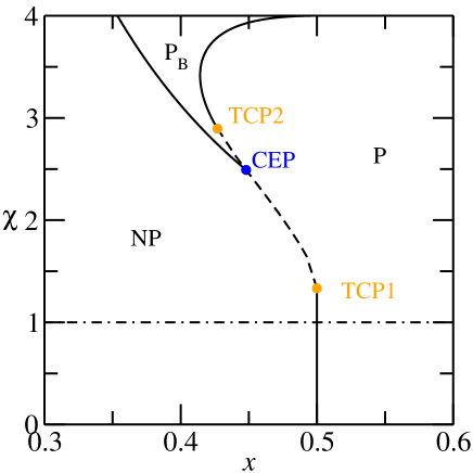
Figure 10: (Color online) Phase diagram for $x_{1}=x_{2}=x$ and $q=3$. Two tricritical points (orange) and a critical end point (blue) shown.

V Conclusion

As shown above, the phase diagram of polymers placed on a bilayer with first neighbor interactions between bonds in different layers displays a variety of critical surfaces and multicritical lines and points, due to the fact that one non-polymerized and four distinct polymerized phases appear. Although to our knowledge such a system has not yet be studied experimentally, it is possible that an experimental situation similar to the model we study here may be found, with polymers confined to a region close to the interfaces between immiscible liquids, for example. Also, due to the richness of the phase diagram of the model associated with the relative simplicity of its solution of the Bethe lattice, which even allows one to obtain many features of the thermodynamic behavior analytically, we believe this model to have also some pedagogical interest for explaining multicritical points.

As discussed in the introduction, magnetic bilayers have been much studied in the literature by a variety of theoretical methods, including pairs of Bethe lattices similar to what was done above albayrak , and, as was discussed in the introduction, polymer models may be mapped onto ferromagnetic $n$-vector models in the limit $n\to 0$. This correspondence may be generalized along the lines proposed for equilibrium polymerization in poor solvents wp81b , and in a particular limit may map into an effective $n\to 0$-vector model with higher order spin interactions between spins in distinct layers, and therefore it may be possible that similar phase diagrams to the ones found here may appear in related magnetic models, even for other values of $n$. Thus, there exists a possibility that phase diagrams similar to the ones found here may appear in appropriate magnetic bilayers.

We notice that in all phase diagrams, with the exception of the first one shown in figure 3, the most interesting features, such as multicritical loci, appear in the region of parameters where the interaction between bonds is attractive ($\chi>1$), and this corresponds to the effective models for polymers in poor solutions mentioned in the introduction.

Although we did not present here in detail the results for the model with interactions between monomers, in the particular case $\kappa=1$ where we compared both models it is already apparent that the results are qualitatively different. This may be seen as rather surprising at first, but, as mentioned above, happens for SASAW’s in two-dimensional lattices mos01 and for Husimi lattices built with squares sms96 , where a saturated polymerized phase is stable in a region of the parameter phase for the model with interactions between bonds. The attractive interactions between bonds and monomers both favor more compact polymerized phases, but the details of these phases and the phase diagram may be quite different for both models. The richness of the phase diagram of polymers on bilayers is quite impressive, four distinct polymerized phases appear, and this gives rise to a variety of phase transition and multicritical loci.

- (1) P. J. Flory, Principles of Polymer Chemistry, edition, Cornell University Press, NY (1966).
- (2) P. G. de Gennes, Scaling Concepts in Polymer Physics, Cornell University Press, NY (1979).
- (3) P. G. de Gennes, Phys. Lett. A 38,339 (1972).
- (4) J. C. Wheeler and P. Pfeuty, Phys. Rev. A 24, 1050 (1981).
- (5) P. G. de Gennes, J. Physique Lettres 36, 1049 (1975).
- (6) S. Kumar and Y. Singh, J. Phys A 26, L987 (1993).
- (7) S. Kumar and Y. Singh, Phys. Rev. E 51, 579 (1995).
- (8) H. W. J. Blöte and B. Nienhuis, J. Phys. A 22 , 1415 (1989); M. T. Batchelor, B. Nienhuis, and S. O. Warnaar, Phys. Rev. Lett. 62, 2425 (1989); B. Nienhuis, Physica (Amsterdam) 163A, 152 (1990).
- (9) J. C. Wheeler and P. Pfeuty, J. Chem. Phys. 74, 6415 (1981).
- (10) J. F. Stilck, K. D. Machado, and P. Serra, Phys. Rev. Lett. 76, 2734 (1996). See also M. Pretti, Phys. Rev. Lett. 89, 1169601 (2002).
- (11) K. D. Machado, M. J. de Oliveira, and J. F. Stilck, Phys. Rev. E 64, 051810 (2001); D. P. Foster, J. Phys. A 40, 1963 (2007).
- (12) M. N. Baibich et al. , Phys. Rev. Lett. 61, 2472 (1988); J. Unguris, R. J. Celotta, and D. T. Pierce, ibid. 67, 140 (1991); S. S. P. Parkin, N. More, and K. P. Roche 64, 2304 (1990).
- (13) M. L. Lyra and C. R. da Silva, Phys. Rev. B 46, 3420 (1992).
- (14) O. Canko and E. Albayrak Phys. Rev. E 75, 011116 (2007); E. Albayrak and S. Yilmaz, J. Phys. Condensed Matter 19, 376212 (2007); E. Albayrak, A. Yigit and S. Akkaya, J. Magn. Magn. Mater. 310, 98 (2007); E. Albayrak, A. Yigit and S. Akkaya, J. Magn. Magn. Mater. 320, 2241 (2008); E. Albayrak and S. Akkaya, Physica Scripta 79, 065005 (2009).
- (15) A. Halperin and P. Pincus, Macromol. 19, 79 (1986)
- (16) Z.-G. Wang, A. M. Nemirovski, and K. F. Freed, J. Chem. Phys. 85, 3068 (1986).
- (17) A. V. Ermoshkin, J. Z. Y. Chen and P. Y. Lai, Phys. Rev. E 66, 051912 (2002).
- (18) R. Baxter, Exactly Solved Models in Statistical Mechanics, (Academic Press, London, 1982).
- (19) P. Serra and J. F. Stilck, J. Phys. A 23, 5351 (1990).
- (20) P. Serra and J. F. Stilck, Phys. Rev. E 75, 011130 (2007).
- (21) P. D. Gujrati, Phys. Rev. Lett. 74, 809 (1995).
- (22) T. J. Oliveira, J.F. Stilck and P. Serra, Phys. Rev. E 80, 041804 (2009).
- (23) A. D. Bruce and A. Aharony, Phys. Rev. B 11, 478 (1975); M. E. Fisher and D. R. Nelson, Phys. Rev. Lett. 32, 1350 (1974).
- (24) J. E. Kirkham, J. Phys. A: Math. Gen 14, L437 (1981).