Holomorphic orbidiscs and Lagrangian Floer cohomology of symplectic toric orbifolds

Abstract.

We develop Floer theory of Lagrangian torus fibers in compact symplectic toric orbifolds. We first classify holomorphic orbi-discs with boundary on Lagrangian torus fibers. We show that there exists a class of basic discs such that we have one-to-one correspondences between a) smooth basic discs and facets of the moment polytope, and b) between basic orbi-discs and twisted sectors of the toric orbifold. We show that there is a smooth Lagrangian Floer theory of these torus fibers, which has a bulk-deformation by fundamental classes of twisted sectors of the toric orbifold. We show by several examples that such bulk-deformation can be used to illustrate the very rigid Hamiltonian geometry of orbifolds. We define its potential and bulk-deformed potential, and develop the notion of leading order potential. We study leading term equations analogous to the case of toric manifolds by Fukaya, Oh, Ohta and Ono.

1. Introduction

The Floer theory of Lagrangian torus fibers of symplectic toric manifolds has been studied very extensively in the last decade, starting from the case of $\mathbb{CP}^{n}$ in [C1] and the toric Fano case in [CO]. These are based on the Lagrangian Floer theory ([Fl], [O1],[O2]), whose general construction was developed by Fukaya, Oh, Ohta and Ono [FOOO]. More recent works [FOOO2],[FOOO3], [FOOO4] have used the (bulk) deformation theory developed in [FOOO], bringing deep understanding of the theory in toric manifolds, and providing beautiful pictures of (homological) mirror symmetry and symplectic dynamics.

We develop an analogous theory for compact symplectic toric orbifolds in this paper. Namely, this paper can be regarded as an orbifold generalization of [C1], [CO], [FOOO2] [FOOO3]. We will see that the main framework is very similar, but that the characteristics of the resulting Floer theory for toric orbifolds are somewhat different than those of toric manifolds.

The main new ingredient is the orbifold $J$-holomorphic disc (called orbi-disc). These are $J$-holomorphic discs with orbifold singularity in the interior. The study of toric manifolds has illustrated that understanding holomorphic discs is a crucial step in developing Lagrangian Floer theory. The holomorphic discs can be used to define the potential, corresponding to the Landau-Ginzburg superpotential for the mirror and the potential essentially computes the Lagrangian Floer cohomology of the torus fibers. Holomorphic discs (which are non-singular) were classified in [CO]. We find a classification for holomorphic orbi-discs in section 6.

One of the main observations of this paper is that the orbifold Lagrangian Floer theory should be considered in the following way. Let us consider a Lagrangian submanifold $L$ which lies in the smooth locus of a symplectic orbifold $\mathcal{X}$. Then, there is a Lagrangian Floer theory of $L$ which only considers, maps from smooth(non-orbifold) (stable) bordered Riemann surfaces. (Here smooth means that there is no orbifold singularity, but it could be a nodal Riemann surface.) Namely, there is a smooth Lagrangian Floer cohomology, and smooth $A_{\infty}$-algebra of $L$, by considering smooth $J$-holomorphic discs and strips. We remark that smooth $J$-holomorphic discs can meet orbifold locus if it has correct multiplicity around the orbifold point, as will be seen in the basic discs later.

Then, the new ingredients, orbifold $J$-holomorphic strips, and discs, enter into the theory in the form of bulk deformation of the smooth Floer theory. Bulk deformation was introduced in [FOOO] to deform the given Lagrangian Floer theory by an ambient cycle in the symplectic manifold. Orbifold $J$-holomorphic strips and discs can be considered to give bulk deformations from the fundamental cycles of twisted sectors of the symplectic orbifold $\mathcal{X}$. In the case of manifolds, the bulk deformation utilizes the already existing $J$-holomorphic discs in the Floer theory, but for orbifolds, the orbifold strips and discs do not exist in the smooth Floer theory. We observe that the mechanism of bulk deformation by orbifold maps captures the very rigid Hamiltonian geometry of symplectic orbifolds.

As noted in [Wo], [WW], [ABM], the dynamics of Hamiltonian vector fields in symplectic orbifolds are quite restrictive. This is because the induced Hamiltonian diffeomorphism should preserve the isomorphism type of the points in the given orbifold. This phenomenon can be easily seen in the example of teardrop orbifold which will be explained later in this introduction. For example, in [FOOO2] or [FOOO3], Fukaya, Oh, Ohta and Ono find locations of non-displaceable Lagrangian torus fibers in toric manifolds, which turn out to be always codimension one or higher in the corresponding moment polytopes. For toric orbifolds, already in the case of teardrop orbifold, we find codimension 0 locus of non-displaceable fibers, and we will find in Proposition 15.2 that if all the points in the toric divisors have orbifold singularity, then in fact all Lagrangian torus fibers are non-displaceable. It is quite remarkable that this phenomenon can be explained as a flexibility to choose bulk deformation coefficient in the leading order potential, which is essentially due to the fact that the orbifold discs and strips do not appear in the smooth Lagrangian Floer theory.

We remark that the non-displaceability of torus orbits in toric orbifolds such as discussed in our examples has been recently proved by Woodward [Wo], Wilson-Woodward [WW] using gauged Floer theory, which is somewhat different from our methods. Their work is roughly based on holomorphic discs in $\mathbb{C}^{m}$ and gauged theory for symplectic reduction. But note that the actual bulk orbi-potentials defined in this paper cannot be defined using their methods, as orbifold discs with more than one orbifold marked point do not come from discs in $\mathbb{C}^{m}$. Also the formalism of bulk deformation developed in this paper seems to give more intuitive understanding of these non-displaceabililty results in orbifolds, which should generalize to a non-toric setting.

Beyond the symplectic dynamics of the toric orbifolds, the development of this theory can be meaningful in the following aspects. First, it provides basic ingredients to study (homological) mirror symmetry([Ko]) of toric orbifolds. In [FOOO4], mirror symmetry of toric manifolds has been proved using Lagrangian Floer theory of toric manifolds. It is easy to see that the similar formalism may be used to explain mirror symmetry of toric orbifolds, which we leave for future research.

Second, the study of orbifold $J$-holomorphic discs provides a new approach to study the crepant resolution conjecture, which relates the invariants of certain orbifolds and its crepant resolutions. In a joint work of the first author, with K. Chan, S.C. Lau, H.H. Tseng, we will formulate an open version of the crepant resolution conjecture for toric orbifolds, and we find a geometric explanation for the change of variable in Kähler moduli spaces of a toric orbifold and its crepant resolution. Also, this provides a natural explanation of specialization to the root of unity in the crepant resolution conjecture, in terms of associated potential functions.

Now, we explain the basic setting and results of the paper in more detail. Compact symplectic toric orbifolds have one-to-one correspondence with labeled polytopes $(P,\vec{c})$, as explained by Lerman and Tolman [LT]. Here $P$ is a simple rational polytope equipped with positive integer labels $\vec{c}$ for each facet. Also the underlying complex orbifold may be obtained from the stacky fan of Borisov, Chen and Smith [BCS]. Stacky fan is a simplicial fan in a finitely generated $\mathbb{Z}$-module $N$ with a choice of lattice vectors in one dimensional cones. A stacky fan corresponds to a toric orbifold when the module $N$ is freely generated. The moment map $\mu_{T}$ exists for the Hamiltonian torus action on a symplectic toric orbifold, and each Lagrangian $T^{n}$ orbit is given by $L(u)=\mu_{T}^{-1}(u)$ for an interior point $u\in P$.

We recall that orbifolds are locally given as quotients of Euclidean space with a finite group action, and the study of Gromov-Witten theory has been extended to the case of orbifolds in the last decade, starting from the work of Chen and Ruan in [CR]. In particular, they have introduced $J$-holomorphic maps from orbi-curves to an almost complex orbifold and have shown that a moduli space of such $J$-holomorphic maps of a fixed type has a Kuranishi structure and a virtual fundamental cycle, hence can be used to define Gromov-Witten invariants.

To find holomorphic orbi-discs with boundary on $L(u)$, we first define what we call the desingularized Maslov index for J-holomorphic orbi-discs. This is done using the desingularization of the pull-back orbi-bundle introduced in [CR]. The standard Maslov index cannot be defined here since the pull-back tangent bundle is not a vector bundle but an orbi-bundle. (See [CS] for related results). We then establish a desingularized Maslov index formula in terms of intersection numbers with toric divisors (analogous to [C1], [CO]).

There is a class of holomorphic (orbi)-discs, which play the role of Maslov index two discs in the smooth cases. We call them basic discs, and they are either smooth holomorphic discs of Maslov index two, or holomorphic orbi-discs with one orbifold marked point, of desingularized Maslov index zero. These basic discs are relevant for the computation of Floer cohomology of Lagrangian torus fibers. We find that there exist holomorphic orbi-discs corresponding to each non-trivial twisted sector of the toric orbifold, which are basic. In addition, we find the area formula of the basic orbi-discs and prove their Fredholm regularity.

We can use smooth $J$-holomorphic discs to set up smooth $A_{\infty}$-algebra for a Lagrangian torus fiber $L$, and its smooth potential function $PO(b)$ for bounding cochains $b\in H^{1}(L;\Lambda_{0})$ in the same way as in [FOOO2]. This potential $PO(b)$ can be used to compute smooth Lagrangian Floer cohomology for $L$, by considering its critical points. The leading order potential of $PO(b)$ is in fact, what is usually called Hori-Vafa Landau-Ginzburg superpotential of the mirror [HV].

Now, as explained above, we can use orbifold $J$-holomorphic discs and strips to set up bulk deformation of the above smooth Lagrangian Floer theory, following [FOOO3]. The bulk deformed $A_{\infty}$-algebra gives rise to a bulk deformed potential $PO^{\mathfrak{b}}(b)$, which is a bulk deformation of the potential $PO(b)$ above. The leading order potential of $PO^{\mathfrak{b}}(b)$, which we denote by $PO^{\mathfrak{b}}_{orb,0}(b)$ can be explicitly written down from the classification results on basic (orbi)-discs.

Note that full bulk-deformed potential $PO^{\mathfrak{b}}(b)$ is difficult to compute, but the leading order potential $PO^{\mathfrak{b}}_{orb,0}(b)$ given in (1.1) can be used to determine non-displaceable Lagrangian torus fibers, by studying the corresponding leading term equation of $PO^{\mathfrak{b}}_{orb,0}(b)$ as in [FOOO3].

More precisely, consider the bulk deformation term $\mathfrak{b}=\mathfrak{b}_{sm}+\mathfrak{b}_{orb}$ given by

$$\begin{cases}\mathfrak{b}_{sm}=\sum_{i=1}^{m}\mathfrak{b}_{i}D_{i}&\mathfrak{b}_{i}\in\Lambda_{+}\\ \mathfrak{b}_{orb}=\sum_{\nu\in Box^{\prime}}\mathfrak{b}_{\nu}1_{\mathcal{X}_{\nu}}&\mathfrak{b}_{\nu}\in\Lambda_{+}.\end{cases}$$ (1.1)

Here, $D_{i}$’s are toric divisors, and $1_{\mathcal{X}_{\nu}}$ are fundamental classes of twisted sectors.

Leading order potential $PO^{\mathfrak{b}}_{orb,0}$ is explicitly defined as

$$PO^{\mathfrak{b}}_{orb,0}=z_{1}+\cdots+z_{m}+\sum_{\nu\in Box^{\prime}}\mathfrak{b}_{\nu}z^{\nu}$$ (1.2)

Here $\nu=\sum_{i=1}^{m}c_{i}\boldsymbol{b}_{i}\in N$ so that $z^{\nu}$ is well-defined Laurent polynomial of $y_{1},\cdots,y_{n}$, $y^{-1},\cdots,y_{n}^{-1}$.

It is important to note that the leading order potential $PO(b)_{0}$, in the case of toric manifolds, is independent of bulk parameter $\mathfrak{b}$, but in our case, $PO^{\mathfrak{b}}_{orb,0}$ depends on the choice of $\mathfrak{b}_{\nu}$. In particular, this term provides a freedom to choose appropriate values, and different choice of $\mathfrak{b}_{\nu}$ will change the leading term equation.

The construction of $A_{\infty}$-algebra, and its bulk-deformation, and those of $A_{\infty}$-bimodules for a pair of Lagrangian submanifolds, and the related isomorphism between the Floer cohomology of bimodule and of $A_{\infty}$-algebra are almost the same as that of [FOOO2], and [FOOO3]. To keep the size of the paper reasonable, we only explain how to adapt their constructions in our cases.

To illustrate the results of this paper, we explain the conclusions of the paper in the case of a teardrop orbifold $P(1,3)$. The teardrop example is explained in more detail in section 15.1.

Figure 1. Teardrop

The teardrop orbifold has an orbifold singularity at the north pole $N$, with isotropy group $\mathbb{Z}/3$. The moment map $\mu_{T}$ has an image given by an interval $[-1/3,1]$, and we put integer label $3$ at the vertex $(-1/3)$. The inverse image $\mu_{T}^{-1}([-1/3,0))$ defines an open neighborhood $U_{N}$ of the north pole $N$, with a uniformizing cover $\widetilde{U}_{N}\cong D^{2}$ with $\mathbb{Z}/3$-action. The inverse image of $\mu_{T}^{-1}((0,1])$ defines a neighborhood $U_{S}$ of the south pole $S$. The length for $U_{N}$ is one third of that of $U_{S}$, since the symplectic area of $U_{N}$ should be considered as that of one third of the uniformizing cover $D^{2}$. Hamiltonian function $H$ is an invariant function on $\widetilde{U}_{N}$ near $U_{N}$, and hence $N$ is a critical point of such $H$.Thus any Hamiltonian flow fixes $N$, and a nearby circle fiber cannot be displaced from itself as illustrated in the Figure. But the fiber $\mu_{T}^{-1}(u)$ for $u>1/3$ can be displaced in the open set $P(1,3)\setminus\{N\}$. Thus the fibers $\mu_{T}^{-1}(u)$ for $u\in(-1/3,1/3]$ are non-displaceable as shown in [Wo]. This is a prototypical example of Hamiltonian rigidity in symplectic orbifolds.

As explained in more detail in section 15.1, such non-displaceability can be proved using our methods. First, the (central) fiber $\mu_{T}^{-1}(0)$ can be shown to be non-displaceable using smooth Lagrangian Floer theory, since the two smooth holomorphic discs (of Maslov index two) with boundary on $\mu_{T}^{-1}(0)$ has the same symplectic area and cancels each other in the Floer differential. This is because that the smooth disc wraps around $U_{N}$ three times, which then has the same symplectic area as the smooth disc covering $U_{S}$.

Then, if we introduce bulk deformation by twisted sectors, then we can show that fibers $\mu_{T}^{-1}(u)$ for $u\in(-1/3,1/3]$ are indeed non-displaceable. Namely, instead of cancelling smooth discs covering upper and lower hemisphere, we can cancel the smooth disc covering $U_{S}$ with one of the orbi-disc of $N$. Their symplectic areas do not match, but as the orbi-discs appear as bulk-deformations, we can adjust the coefficient $\mathfrak{b}_{\nu}$ to match their areas using our freedom to choose such coefficients. Note that this method does not work for the fibers with $u\in(1/3,1)$ since the areas of orbi-discs are bigger than that of the smooth disc covering $S$, and since $\mathfrak{b}_{\nu}$ should lie in $\Lambda_{+}$.

Acknowledgement:

First author would like to thank Kaoru Ono for the comment regarding the Proposition 15.2 and Siu-Cheong Lau for helpful discussions on orbi-potentials, and Kwokwai Chan for helpful comments on the draft. Part of the paper is written in the first author’s stay at Northwestern University as a visiting professor, and he would like to thank them for their hospitality. The second author thanks Seoul National University for its hospitality on many occasions. He also thanks Bernardo Uribe and Andres Angel for discussions on related topics.

Notation:

Throughout the paper, $\mathcal{X}$ is an orbifold and $X$ is the underlying topological space. We denote by $I\mathcal{X}$ the inertia orbifold, $T=\{0\}\cup T^{\prime}$, the index set of inertia components. We denote by $\iota_{\nu}$ the rational number called age or degree shifting number associated to each connected component $\mathcal{X}_{\nu}$. For toric orbifolds, we will identify $T$ and denote it as $Box$ in definition 4.1.

The lattice $N\cong\mathbb{Z}^{n}$ parametrizes the one parameter subgroups of the group $(\mathbb{C}^{\ast})^{n}$. Let $M$ be its dual lattice. $\Sigma$ is a rational simplicial polyhedral fan in $N_{\mathbb{R}}$, and $P\subset M_{R}$ is a rational convex polytope.

The minimal lattice vectors perpendicular to the facets of $P$, pointing toward the interior are denoted by $\boldsymbol{v}_{1},\cdots,\boldsymbol{v}_{m}$. Certain integral multiples $\boldsymbol{b}_{j}=c_{j}\boldsymbol{v}_{j}$ will be called stacky vectors.

For $u\in M_{\mathbb{R}}$, let

$$\ell_{j}(u)=\langle u,\boldsymbol{b}_{j}\rangle-\lambda_{j}.$$ (1.3)

Then the moment polytope $P$ and its boundary are given by

$$P=\{u\in M_{\mathbb{R}}\mid\ell_{i}(u)\geq 0,i=1,\cdots,m\},\;\;\partial_{i}P=\{u\in M_{\mathbb{R}}\mid\ell_{i}(u)=0\}.$$

Here $\partial_{i}P$ is the $i$-th facet of the polytope $P$.

Let $\mu_{T}:X\to P$ be the moment map. Consider $u\in Int(P)$ and denote $L(u)=\mu_{T}^{-1}(u)$. We may write $L$ instead of $L(u)$ to simplify notations.

We will consider the coefficient ring $R$ to be $\mathbb{R}$ (as we work in de Rham model of $A_{\infty}$-algebra) or $\mathbb{C}$ (when finding the critical point of the potential). To emphasize the choice of coefficient ring $R$ in the Novikov ring below, we may write $\Lambda^{R},\Lambda^{R}_{0}$ instead of $\Lambda,\Lambda_{0}$.

Universal Novikov ring $\Lambda$ and $\Lambda_{0}$ is defined as

$$\Lambda = \{\sum_{i=1}^{\infty}a_{i}T^{\lambda_{i}}\mid a_{i}\in R,\lambda_{i}\in\mathbb{R},\lim_{i\to\infty}\lambda_{i}=\infty\},$$ (1.4)

$$\Lambda_{0} = \{\sum_{i=1}^{\infty}a_{i}T^{\lambda_{i}}\in\Lambda\mid\lambda_{i}\in\mathbb{R}_{\geq 0}\}.$$ (1.5)

$$\Lambda_{+} = \{\sum_{i=1}^{\infty}a_{i}T^{\lambda_{i}}\in\Lambda\mid\lambda_{i}>0\}.$$ (1.6)

In [FOOO], the universal Novikov ring $\Lambda_{0,nov}$ is defined as

$$\Lambda_{0,nov}=\left.\left\{\sum_{i=1}^{\infty}a_{i}T^{\lambda_{i}}e^{n_{i}}\,\,\right|\,\,a_{i}\in R,n_{i}\in\mathbb{Z},\lambda_{i}\in\mathbb{R}_{\geq 0},\lim_{i\to\infty}\lambda_{i}=\infty\right\}.$$ (1.7)

This is a graded ring by defining $\deg T=0$, $\deg e=2$. and $\Lambda_{nov}$ and $\Lambda_{0,nov}^{+}$ can be similarly defined. By forgetting $e$ from $\Lambda_{0,nov}$ and working with $\Lambda_{0}$, we can only work in $\mathbb{Z}_{2}$ graded complex.

We define a valuation $\mathfrak{v}_{T}$ on $\Lambda$ by

$$\mathfrak{v}_{T}(\sum_{i=0}^{\infty}a_{i}T^{\lambda_{i}})=\textrm{inf}\{\lambda_{i}\mid a_{i}\neq 0\}.$$

It is unfortunate but due to the convention, three b’s, written as $b,\mathfrak{b},\boldsymbol{b}$ will be used throughout the paper, each of which has a different meaning. Here $\boldsymbol{b}_{j}$ is the stacky normal vector to $j$-th facet of the polytope, $b=\sum x_{i}e_{i}$ denotes a bounding cochain in $H^{1}(L,\Lambda_{0})$, and $\mathfrak{b}$ denotes the bulk bounding cochain.

2. $J$-holomorphic discs and moduli space of bordered stable maps

In this section, we discuss moduli spaces of isomorphism classes of stable maps from a genus $0$ prestable bordered Riemann surfaces with Lagrangian boundary condition together with interior orbifold marked points of a fixed type. Let $(\mathcal{X},\omega,J)$ be a symplectic orbifold with a compatible almost complex structure. Let $L\subset\mathcal{X}$ be a Lagrangian submanifold (in the smooth part of $\mathcal{X}$).

An orbifold Riemann surface $\boldsymbol{\Sigma}$ is a Riemann surface $\Sigma$ ( with complex structure $j$) together with the orbifold points $z_{1},\cdots,z_{k}\in\Sigma$ such that each orbifold point $z_{i}\in\Sigma$ has a disc neighborhood $U$ of $z_{i}$ which is uniformized by a branched covering map $br:z\to z^{m_{i}}$. We set $m=1$ for smooth points $z\in\Sigma$. If $\Sigma$ has a non-trivial boundary, we always assume that $\partial\Sigma$ is smooth, and that orbifold points lie in the interior of $\Sigma$ and such $\boldsymbol{\Sigma}$ will be called bordered orbifold Riemann surface. Hence $\boldsymbol{\Sigma}$ can be written as $(\Sigma,\vec{z},\vec{m})$ for short.

Definition 2.1.

Let $\boldsymbol{\Sigma}$ be an (bordered) orbifold Riemann surface.

A continuous map $f:\Sigma\to\mathcal{X}$ is called pseudo-holomorphic if for any $z_{0}\in\Sigma$, the following holds:

1. There is a disc neighborhood of $z_{0}$ with a branched covering $br:z\to z^{m}$.

2. There is a local chart $(V_{f(z_{0})},G_{f(z_{0})},\pi_{f(z_{0})})$ of $\mathcal{X}$ at $f(z_{0})$ and a local lifting $\widetilde{f}_{z_{0}}$ of $f$ in the sense that $f\circ br=\pi_{f(z_{0})}\circ\widetilde{f}_{z_{0}}$.

3. $\widetilde{f}_{z_{0}}$ is pseudo-holomorphic.

4. If $\partial\Sigma\neq 0$, the map $f$ satisfies the boundary condition $f(\partial X)\subset L$.

We need a few technical lemmas following [CR] regarding orbifold maps, and we refer readers to the Appendix or [CR] for more details.

Definition 2.2.

A $C^{\infty}$ map ${\bf f}:\boldsymbol{\Sigma}\to\mathcal{X}$ is called regular if $f^{-1}(\mathcal{X}_{reg})$ is an open dense and connected subset of $X$.

Lemma 2.1.

If $\boldsymbol{\Sigma}$ is an bordered orbifold Riemann surface and ${\bf f}:\boldsymbol{\Sigma}\to\mathcal{X}$ is regular and pseudo-holomorphic with Lagrangian boundary condition, then it is the unique germ of $C^{\infty}$ liftings of $f$. Moreover ${\bf f}$ is good with a unique isomorphism class of compatible systems.

Lemma 2.1 may be proved using the main idea of Lemma 4.4.11 in [CR] together with the result on the local behavior of a pseudo-holomorphic map from a Riemann surface near a singularity in the image, given in Lemma 2.1.4 of [CR]. This latter result yields unique continuity of a local lift of a pseudo-holomorphic map near a singularity in the target.

Lemma 2.2.

Suppose $f:\boldsymbol{\Sigma}\to{\mathcal{X}}$ is a pseudo-holomorphic map with interior marked points ${\vec{z}^{+}}=(z_{1}^{+},\ldots,z_{k}^{+})$, such that $f(\partial\Sigma)$ does not intersect the singular set of ${\mathcal{X}}$. Then there exist a finite number of orbifold structures on $\Sigma$ with singular set contained in ${\vec{z}^{+}}$, for which there are good $C^{\infty}$ maps covering $f$. Moreover for each such orbifold structure there exist a finite number of pairs $({\bf f},\xi)$ where ${\bf f}$ is a good map lifting $f$ and $\xi$ is an associated isomorphism class of compatible systems. The number of such pairs is bounded above by a constant that depends on ${\mathcal{X}}$, the genus of $\Sigma$ and $k$ only.

The proof of the above lemma is very similar to Chen-Ruan’s proof in the case without boundary, see Proposition 2.2.1 in [CR]. Simply note that the homomorphisms $\theta_{\xi_{0},\xi_{1}}$ and $\theta_{\xi}$ of [CR] are well defined in our case by an application of Lemma 16.1.

The construction of the moduli space is a combination of the construction of Fukaya, Oh, Ohta and Ono [FOOO] regarding Lagrangian boundary condition, and that of Chen-Ruan [CR] regarding the interior orbifold singularities.

We recall the definition of genus 0 prestable bordered Riemann surfaces from [FOOO].

Definition 2.3.

$\Sigma$ is called a genus 0 prestable bordered Riemann surface if $\Sigma$ is a possibly singular Riemann surface with boundary $\partial\Sigma$ such that the double $\Sigma\cup_{\partial\Sigma}\overline{\Sigma}$ is a connected and simply connected compact singular Riemann surface whose singularities are only nodes. $(\Sigma,\vec{z},\vec{z}^{+})$ is called a genus 0 prestable bordered Riemann surface with $(k,l)$ marked points if $\Sigma$ is a genus 0 prestable bordered Riemann surface and $\vec{z}=(z_{0},\cdots,z_{k-1})$ are boundary marked points on $\partial\Sigma$ away from the nodes, and $\vec{z}^{+}=(z_{1}^{+},\cdots,z_{l}^{+})$ are interior marked points in $\Sigma\setminus\partial\Sigma$.

A genus $0$ prestable bordered Riemann surface $(\Sigma,\vec{z},\vec{z}^{+})$ is said to be stable if each sphere component has three special(nodal or marked) points and each disc component $\Sigma_{\nu}$ satisfies $2l_{\nu}+k_{\nu}\geq 3$ where $l_{\nu}$ is the number of interior special points and $k_{\nu}$ is the number of boundary special points. We denote by $\mathcal{M}_{k,l}$ the space of isomorphism classes of genus 0 stable bordered Riemann surfaces with $(k,l)$ marked points. From the cyclic ordering of the boundary marked points, $\mathcal{M}_{k,l}$ has $(k-1)!$ connected components. The main component $\mathcal{M}_{k,l}^{main}$ is defined by considering a subset of curves in $\mathcal{M}_{k,l}$ whose the boundary marked points are ordered in a cyclic counterclockwise way (for some parametrization of $\partial\Sigma$ as $S^{1}$ for stable case).

We give the definition of genus $0$ prestable bordered orbi-curve following [CR] and [FOOO].

Definition 2.4.

$(\boldsymbol{\Sigma},\vec{z},\vec{z}^{+})$ is called a genus $0$ prestable bordered orbi-curve (with interior singularity) with $(k,l)$ marked points if $(\Sigma,\vec{z},\vec{z}^{+})$ is genus $0$ prestable bordered Riemann surface with $(k,l)$ marked points with the following properties:

1. Orbifold points are contained in the set of interior marked points and interior nodal points.

2. A disc neighborhood of an interior orbifold marked point $z_{i}^{+}$ is uniformized by a branched covering map $z\mapsto z^{m_{i}}$.

3. A neighborhood of interior nodal point(which is away from $\partial\Sigma$) is uniformized by $(X(0,r_{j}),\mathbb{Z}_{n_{j}})$.

Recall from [CR] that the local model of the interior orbifold nodal point, $(X(0,r_{j}),\mathbb{Z}_{n_{j}})$, is defined as follows: For any real number $t\geq 0,r>0$, set $X(t,r)=\{(x,y)\in\mathbb{C}^{2}|\;||x||,||y||<r,xy=t\}$. Fix an action of $\mathbb{Z}_{m}$ on $X(t,r)$ for any $m>1$ by $e^{2\pi i/m}\cdot(x,y)=(e^{2\pi i/m}x,e^{-2\pi i/m}y)$. The branched covering map $X(t,r)\to X(t^{m},r^{m})$ given by $(x,y)\to(x^{m},y^{m})$ is $\mathbb{Z}_{m}$-invariant. So $(X(t,r),\mathbb{Z}_{m})$ can be regarded as a uniformizing system of $X(t^{m},r^{m})$. Here $m_{i},n_{j}$ are allowed to take the value one, in which case the corresponding orbifold structure is trivial. Hence, a data of genus 0 prestable bordered orbi-curve includes the numbers $m_{i},n_{j}$ but we do not write them for simplicity. A notion of isomorphism and the group of automorphisms of genus 0 prestable bordered orbi-curves with interior singularity is defined in a standard way, and omitted.

Now we define orbifold stable map to be used in this paper. We write $\Sigma=\bigcup_{\nu}\Sigma_{\nu}$ for each irreducible component $\Sigma_{\nu}$.

Definition 2.5.

A genus 0 stable map from a bordered orbi-curve with $(k,l)$ marked points is a pair $\big{(}(\boldsymbol{\Sigma},\vec{z},\vec{z}^{+}),w,\xi\big{)}$ satisfying the following properties:

1. $(\boldsymbol{\Sigma},\vec{z},\vec{z}^{+})$ be a genus 0 prestable bordered orbi-curve

2. $w:(\Sigma,\partial\Sigma)\to(\mathcal{X},L)$ is a pseudo-holomorphic map (see Definition 2.1). (Here, we say that $w$ is pseudo-holomorphic (resp. good) if each $w_{\nu}$ is pseudo-holomorphic (resp. good) and induce a continuous map $w:\Sigma\to X$.)

3. $w$ is a $C^{\infty}$ good map with an isomorphism class $\xi$ of compatible systems.

4. $w$ is representable i.e. it is injective on local groups.

5. The set of all $\phi:\Sigma\to\Sigma$ satisfying the following properties is finite.

   1. $\phi$ is biholomorphic.

   2. $\phi(z_{i})=z_{i},\phi(z_{i}^{+})=z_{i}^{+}$

   3. $w\circ\phi=w$

Definition 2.6.

Two stable maps $\big{(}(\boldsymbol{\Sigma}_{1},\vec{z}_{1},\vec{z}_{1}^{+}),w_{1},\xi_{1}\big{)}$ and $\big{(}(\boldsymbol{\Sigma}_{2},\vec{z}_{2},\vec{z}_{2}^{+}),w_{2},\xi_{2}\big{)}$ are equivalent if there exists an isomorphism $h:(\boldsymbol{\Sigma}_{1},\vec{z}_{1},\vec{z}_{1}^{+})\to(\boldsymbol{\Sigma}_{2},\vec{z}_{2},\vec{z}_{2}^{+})$ such that $w_{2}\circ h=w_{1}$ and $\xi_{1}=\xi_{2}\circ h$ , i.e. the isomorphism class $\xi_{2}$ pulls back to the class $\xi_{1}$ via $h$.

Definition 2.7.

An automorphism of a stable map $\big{(}(\boldsymbol{\Sigma},\vec{z},\vec{z}^{+}),w,\xi\big{)}$ is a self equivalence. The automorphism group is denoted by $Aut\big{(}(\boldsymbol{\Sigma},\vec{z},\vec{z}^{+}),w,\xi\big{)}$.

Given a stable map $\big{(}(\boldsymbol{\Sigma},\vec{z},\vec{z}^{+}),w,\xi\big{)}$, we associate a homology class $w_{*}([\Sigma])\in H_{2}(X,L)$. Note that for each interior marked point $z^{+}_{j}$ (on $\Sigma_{\nu}$), $\xi_{\nu}$ determines by the group homomorphism at $z^{+}_{j}$, a conjugacy class $(g_{j})$, where $g_{j}\in G_{w(z_{j})}$.

Let $I\mathcal{X}$ be the inertia orbifold of $\mathcal{X}$. Denote by $T=\{0\}\cup T^{\prime}$ the index set of inertia components, and for $(g)\in T$, call the corresponding component $\mathcal{X}_{(g)}$. Here $\mathcal{X}_{(0)}$ is $\mathcal{X}$ itself, and elements of $x\in\mathcal{X}_{(g)}$ are written as $(x,g)$.

We thus have a map $ev_{i}^{+}$ sending each (equivalence class of) stable map into $I\mathcal{X}$ by

$$ev_{i}^{+}:\big{(}(\boldsymbol{\Sigma},\vec{z},\vec{z}^{+}),w,\xi\big{)}\to(w(z^{+}_{i}),g_{i}).$$

Denote by $\underline{l}=\{1,\cdots,l\}$ and consider the map $\boldsymbol{x}:\underline{l}\to T$ describing the inertia component for each (orbifold) marked point. A stable map $\big{(}(\boldsymbol{\Sigma},\vec{z},\vec{z}^{+}),w,\xi\big{)}$ is said to be of type $\boldsymbol{x}$ if for $i=1,\cdots,l$,

$$ev^{+}_{i}\big{(}(\boldsymbol{\Sigma},\vec{z},\vec{z}^{+}),w,\xi\big{)}\in\mathcal{X}_{\boldsymbol{x}(i)}.$$

Definition 2.8.

Given a homology class $\beta\in H_{2}(X,L)$, we denote by $\mathcal{M}_{k,l}(L,J,\beta,\boldsymbol{x})$ the moduli space of isomorphism classes of genus 0 stable maps to $\mathcal{X}$ from a bordered orbi-curve with $(k,l)$ marked points of type $\boldsymbol{x}$ and with $w_{*}([\Sigma])=\beta$. We denote by $\mathcal{M}_{k,l}^{main}(L,J,\beta,\boldsymbol{x})$ the sub-moduli space with $(\boldsymbol{\Sigma},\vec{z},\vec{z}^{+})\in\mathcal{M}_{k,l}^{main}$.

Remark 2.9.

We follow the notations of [FOOO] and denote by $\mathcal{M}$ the compactified moduli space, and by $\mathcal{M}^{reg}$ the moduli space before compactification.

We can give a topology on the moduli space $\mathcal{M}_{k,l}^{main}(L,J,\beta,\boldsymbol{x})$ in a way similar to [FOn],[FOOO] and [CR2] (definition 2.3.7). As it is standard, we omit the details. Following Proposition 2.3.8 and Lemma 2.3.9 of [CR], we have

Lemma 2.3.

The moduli space $\mathcal{M}_{k,l}^{main}(L,J,\beta,\boldsymbol{x})$ is compact and metrizable.

The symplectic area of elements in $\mathcal{M}_{k,l}^{main}(L,J,\beta,\boldsymbol{x})$ only depends on the homology class $\beta$ and the symplectic form $\omega$.

The orientation issues can be dealt exactly in the same way as in [FOOO]. Theorem 2.1.30 together with Proposition 3.3.5 of [CR] show that the Kuranishi structure for orbifold case is stably complex.

Theorem 2.4.

Let $L$ be relatively spin. Then a choice of relative spin structure of $L\subset X$ canonically induces an orientation of $\mathcal{M}_{k,l}^{main}(L,J,\beta,\boldsymbol{x})$.

We will consider the moduli space $\mathcal{M}_{k,l}^{main}(L,\beta,\boldsymbol{x})$ (with $J=J_{0}$ the standard complex structure of the toric orbifolds) in more detail later, but the virtual dimension of the moduli space is given as follows.

Lemma 2.5.

The virtual dimension of the moduli space $\mathcal{M}_{k,l}^{main}(L,\beta,\boldsymbol{x})$ is

$$n+\mu^{de}(\beta,\boldsymbol{x})+k+2l-3\;=\;n+\mu_{CW}(\beta)+k+2l-3-2\iota(\boldsymbol{x}).$$

In the next section, we will explain $\mu^{de}$ which is the desingularized Maslov index of $(\beta,\boldsymbol{x})$, and $\mu_{CW}(\beta)$ which is the Chern-Weil Maslov index of [CS]. Let $\iota(\boldsymbol{x})=\sum_{i}\iota_{(g_{i})}$ for $\boldsymbol{x}=(\mathcal{X}_{(g_{1})},\cdots,\mathcal{X}_{(g_{l})})$ where $\iota_{(g)}$ is the degree shifting number defined by Chen-Ruan [CR2]. We remark that the desingularized Maslov index depends on $\boldsymbol{x}$ as we need to desingularize the pull-back tangent orbi-bundle, which depends on $\boldsymbol{x}$.

3. Desingularized Maslov index

Maslov index is related to the (virtual) dimension of moduli spaces in Lagrangian Floer theory (Lemma 2.5). For orbifolds, the standard definition of Maslov index does not have natural extension, since the pull-back tangent bundle under a good map is usually an orbi-bundle which is not a trivial bundle over the bordered orbi-curve.

In this section, we define, what we call, desingularized Maslov index, and provide computations of several examples of holomorphic orbi-discs, which will appear in later sections. On the other hand, recently, the first author and H.-S. Shin [CS] gave Chern-Weil definition of Maslov index, which is given by curvature integral of an orthogonal connection. This Chern-Weil definition naturally extends to the orbifold setting, and the relation between Chern-Weil and desingularized Maslov indices has been discussed in [CS]. We give a brief explanation at the end of this section.

3.1. Definition of desingularized Maslov index

Chen and Ruan [CR] have shown that for orbifold holomorphic map $u:\boldsymbol{\Sigma}\to\mathcal{X}$ from a closed orbi-curve without boundary to an orbifold, the Chern number $c_{1}(T\mathcal{X})([\boldsymbol{\Sigma}])$ (defined via Chern-Weil theory) is in general a rational number and by suitable subtraction of degree shifting number for each orbifold point, one obtains the Chern number of a desingularized bundle which is an honest bundle. Hence the corresponding number is an integer. It is related to the Fredholm index for the moduli spaces.

The similar phenomenon happens for orbi-discs (discs with interior orbifold singularities). We will mainly work with a Maslov index of a desingularized orbi-bundle and such an index will be called desingularized Maslov index for short, and this will be an integer.

Let us first recall the standard definition of Maslov index for a smooth disk with Lagrangian boundary condition. If $w:(D^{2},\partial D^{2})\to(X,L)$ is a smooth map of pairs, we can find a unique symplectic trivialization (up to homotopy) of the pull-back bundle $w^{*}TX\cong D^{2}\times\mathbb{C}^{n}$. This trivialization defines a map from $S^{1}=\partial D^{2}$ to $(U(n)/O(n))$, the set of Lagrangian planes in $\mathbb{C}^{n}$, and the Maslov index is a rotation number of this map composed with the map $det^{2}:(U(n)/O(n))\to U(1)$ (see [Ar]). For bordered Riemann surfaces with several boundary components, one can define its Maslov index similarly by taking the sum of Maslov indices along $\partial\Sigma$ using the fact that a symplectic vector bundle over a Riemann surface with boundary $\Sigma$ is always trivial. The data of symplectic vector bundle over $\Sigma$, and Lagrangian subbundle over $\partial\Sigma$ is called a bundle pair, and one can define Maslov index for any bundle pair in the same way.

Next, we recall the desingularization of orbi-bundle on an orbifold Riemann surface by Chen and Ruan ([CR]) which plays a key role.

Consider a closed (complex) Riemann surface $\Sigma$, with distinct points $\vec{z}=(z_{1},\cdots,z_{k})$ paired with multiplicity $\vec{m}=(m_{1},\cdots,m_{k})$. We consider the orbifold structure at $z_{i}$ which is given by the ramified covering $z_{i}\to z_{i}^{m_{i}}$. For simplicity we denote it as $\boldsymbol{\Sigma}=(\Sigma,\vec{z},\vec{m})$, which is a closed, reduced, 2-dimensional orbifold.

Consider a complex orbi-bundle $E$ be over $\boldsymbol{\Sigma}$ of rank $n$. Then, at each singular point $z_{i}$, $E$ gives a representation $\rho_{i}:\mathbb{Z}_{m_{i}}\to Aut(\mathbb{C}^{n})$ so that over a disc neighborhood $D_{i}$ of $z_{i}$, $E$ is uniformized by $(D_{i}\times\mathbb{C}^{n},\mathbb{Z}_{m_{i}},\pi)$ where the action of $\mathbb{Z}_{m_{i}}$ on $D_{i}\times\mathbb{C}^{n}$ is defined as

$$e^{2\pi i/m_{i}}\cdot(z,w)=\big{(}e^{2\pi i/m_{i}}z,\rho_{i}(e^{2\pi i/m_{i}})w\big{)}$$ (3.1)

for any $w\in\mathbb{C}^{n}$. Note that $\rho_{i}$ is uniquely determined by integers $(m_{i,1},\cdots,m_{i,n})$ with $0\leq m_{i,j}<m_{i}$, as it is given by the matrix

$$\rho_{i}(e^{2\pi i/m_{i}})=diag(e^{2\pi im_{i,1}/m_{i}},\cdots,e^{2\pi im_{i,n}/m_{i}}\big{)}.$$ (3.2)

The sum $\sum_{j=1}^{n}\frac{m_{i,j}}{m_{i}}$ is called the degree shifting number([CR]).

Over the punctured disc $D_{i}\setminus\{0\}$ at $z_{i}$, $E$ is given a specific trivialization from $(D_{i}\times\mathbb{C}^{n},\mathbb{Z}_{m_{i}},\pi)$ as follows: consider a $\mathbb{Z}_{m_{i}}$-equivariant map $\Psi_{i}:D\setminus\{0\}\times\mathbb{C}^{n}\to D\setminus\{0\}\times\mathbb{C}^{n}$ defined by

$$(z,w_{1},w_{2},\cdots,w_{n})\to(z^{m_{i}},z^{-m_{i,1}}w_{1},\cdots,z^{-m_{i,n}}w_{n}),$$ (3.3)

where $\mathbb{Z}_{m_{i}}$ action on the target $D\setminus\{0\}\times\mathbb{C}^{n}$ is trivial. Hence $\Psi_{i}$ induces a trivialization $\Psi_{i}:E_{D_{i}\setminus\{0\}}\to D_{i}\setminus\{0\}\times\mathbb{C}^{n}$. We may extend the smooth complex vector bundle $E_{\boldsymbol{\Sigma}\setminus\{z_{1},\cdots,z_{k}\}}$ over $\boldsymbol{\Sigma}\setminus\{z_{1},\cdots,z_{k}\}$ to a smooth complex vector bundle over $\boldsymbol{\Sigma}$ by using these trivializations $\Psi_{i}$ for each $i$. The resulting complex vector bundle is called the desingularization of $E$ and denoted by $|E|$.

The essential point as observed in [CR] is that the sheaf of holomorphic sections of the desingularized orbi-bundle and the orbibundle itself are the same.

Proposition 3.1 ([CR] Proposition 4.2.2).

Let $E$ be a holomorphic orbifold bundle of rank $n$ over a compact orbicurve $(\boldsymbol{\Sigma},\boldsymbol{z},\boldsymbol{m})$ of genus $g$. The $\mathcal{O}(E)$ equals $\mathcal{O}(|E|)$, where $\mathcal{O}(E)$ and $\mathcal{O}(|E|)$ are sheaves of holomorphic sections of $E$ and $|E|$.

As the local group action on the fibers of the desingularized orbi-bundle $|E|$ is trivial, one can think of it as a smooth vector bundle on $\Sigma$ which is analytically the same as $\boldsymbol{\Sigma}$ (In other words, there exist a canonically associated vector bundle $|E|$ over the smooth Riemann surface $\Sigma$). Hence, for the bundle $|E|$, the ordinary index theory can be applied, which provides the required index theoretic tools for the orbibundle $E$.

Now we give a definition of the desingularized Maslov index, which determines the virtual dimension of the moduli space of J-holomorphic orbi-discs.

Definition 3.1.

Let $\boldsymbol{\Sigma}=(\Sigma,\vec{z},\vec{m})$ be a bordered orbi-curve with $(0,k)$ marked points. Let $u:\boldsymbol{\Sigma}\to X$ be an orbifold stable map. Then, $u^{*}TX$ is a complex orbi-bundle over $\boldsymbol{\Sigma}$, with Lagrangian subbundle $u|_{\partial\boldsymbol{\Sigma}}^{*}TL$ at $\partial\boldsymbol{\Sigma}$. Let $|u^{*}TX|$ be the desingularized bundle over $\boldsymbol{\Sigma}$( or $\Sigma$), which still have the Lagrangian subbundle at the boundary from $u|_{\partial\Sigma}^{*}TL$. The Maslov index of the bundle pair $(|u^{*}TX|,u|_{\partial\Sigma}^{*}TL)$ over $(\Sigma,\partial\Sigma)$ is called the desingularized Maslov index of $u$, and denoted by $\mu^{de}(u)$. Note that this index is well-defined as it is independent of the choice of compatible system for $u$, within the same isomorphism class, by Lemma 16.1.

3.2. Examples of computations of the index

Here we give a few examples of computations of the desingularized Maslov indices. Consider the orbifold disc $\mathcal{D}$ with $\mathbb{Z}_{p}$ singularity at the origin, and the orbifold complex plane $\boldsymbol{C}$ with $\mathbb{Z}_{p}$ singularity at the origin. Let the unit circle $L=S^{1}\in\boldsymbol{C}$ a Lagrangian submanifold. Consider the natural inclusion $u:\mathcal{D}\to\boldsymbol{C}$.

Lemma 3.2.

The desingularized Maslov index of $u$ equals $0$

Proof.

Consider the tangent orbibundle $T\mathcal{D}$ over $\mathcal{D}$, and its uniformizing chart $D^{2}\times\mathbb{C}=\{(z,w)|z\in D^{2},w\in\mathbb{C}\}$ with the $\mathbb{Z}_{p}$ action given by

$$e^{2\pi i/p}\cdot(z,w)=\big{(}e^{2\pi i/p}z,e^{2\pi i/p}w\big{)}$$ (3.4)

Then, the subbundle $TL$ at $z\in S^{1}$ is given by $\mathbb{R}\cdot iz\subset\mathbb{C}$. We consider its image under the desingularization map $\Psi:D^{2}\times\mathbb{C}\to D^{2}\times\mathbb{C}$ defined as $\Psi(z,w)=(z^{p},z^{-1}w)$. The image of $TL$ via $\Psi$ at the point $\alpha\in D^{2}$ with $\alpha=z^{p}$ is given by $\mathbb{R}\cdot z^{-1}iz=i\cdot\mathbb{R}\subset\mathbb{C}$.

The desingularization provides a desingularized vector bundle over the orbi-disc $\mathcal{D}$, which is a trivial vector bundle, and the loop of Lagrangian subspaces at the boundary is a constant loop. Therefore the desingularized Maslov index is zero. ∎

We now consider a more general case: Consider the orbifold disc $\mathcal{D}$ with $\mathbb{Z}_{m}$ singularity at the origin, and the complex plane $\boldsymbol{C}$ with $\mathbb{Z}_{mn}$ singularity at the origin, and the unit circle $L=S^{1}\in\boldsymbol{C}$ as a Lagrangian submanifold. Consider the uniformizing cover $D^{2}$ of $\mathcal{D}$, with coordinate $z\in D^{2}$. Consider the uniformizing cover $\mathbb{C}$ of $\boldsymbol{C}$, with coordinate $y\in\mathbb{C}$.

Lemma 3.3.

Consider the map $u:\mathcal{D}\to\boldsymbol{C}$, induced from the map $\widetilde{u}:D^{2}\to\mathbb{C}$ defined by $\widetilde{u}(z)=z^{k}$. Here we assume that $k,m$ are relatively prime to ensure that the group homomorphism is injective. Then, the desingularized Maslov index of $u$ equals $2[k/m]$ where $[k/m]$ is the largest integer $\leq k/m$.

Proof.

Consider the tangent orbibundle $T\boldsymbol{C}$ over $\boldsymbol{C}$ whose uniformizing chart is given by $\mathbb{C}\times\mathbb{C}=\{(y,w)|y,w\in\mathbb{C}\}$ with the $\mathbb{Z}_{mn}$ action given by the diagonal action. Then, the subbundle $TL$ at $y\in S^{1}$ is given by $\mathbb{R}\cdot iy\subset\mathbb{C}$. We consider the pull-back orbibundle, $u^{*}T\boldsymbol{C}$ whose uniformizing chart is given by $\mathbb{C}\times\mathbb{C}=\{(z,w)|z,w\in\mathbb{C}\}$ with the $\mathbb{Z}_{m}$ action given by

$$e^{2\pi i/m}\cdot(z,w)=\big{(}e^{2\pi i/m}z,e^{2\pi ki/m}w\big{)}$$ (3.5)

In this chart, the subbundle $(u|_{\partial\mathcal{D}})^{*}TL$ is given by $(z,\mathbb{R}\cdot z^{k}i)$ for $z\in\partial D^{2}$. Now, we consider its image under the desingularization map $\Psi:D^{2}\setminus\{0\}\times\mathbb{C}\to D^{2}\setminus\{0\}\times\mathbb{C}$ defined as $\Psi(z,w)=(z^{m},z^{-k^{\prime}}w)$, where $k^{\prime}=k-[k/m]m$. The image of $TL$ via $\Psi$ at the point $\alpha\in D^{2}$ with $\alpha=z^{m}$ is given by $\mathbb{R}\cdot z^{-k^{\prime}}iz^{k}=z^{[k/m]m}i\cdot\mathbb{R}\subset\mathbb{C}$.

Hence we obtain a trivialized desingularized vector bundle $|E|$ over $\mathcal{D}$( and hence $D^{2}$), and from the above computation, the loop of Lagrangian subspaces along the boundary is given by $z^{[k/m]m}i\cdot\mathbb{R}$. But also note that the coordinate on $D^{2}$ is in fact $z^{m}$, and hence the desingularized Maslov index of $u$ is $2[k/m]$. ∎

Remark 3.2.

Note that in the case that $(k,m)$ are not relatively prime, say $d=gcd(k,m)$, then instead of the map from the above orbifold disc, we consider a domain with simpler singularity, say $\mathcal{D}$ with $\mathbb{Z}_{m/d}$ singularity at the origin, and the map given by $x\mapsto x^{k/d}$. The Maslov index of this orbifold holomorphic disc is still $2[k/m]=2[(k/d)/(m/d)]$.

The following computations of indices will be used later in the paper. We compute desingularized Maslow indices for orbi-discs in $\mathcal{X}=\mathbb{C}^{n}/G$ Consider the orbifold disc $\mathcal{D}$ with $\mathbb{Z}_{m}$ singularity at the origin, and the orbifold $\mathcal{X}$ defined by the complex vector space $\mathbb{C}^{n}$ with an action of a finite abelian group $G$. Consider the uniformizing cover $D^{2}$ of $\mathcal{D}$, with coordinate $z\in D^{2}$.

Lemma 3.4.

Consider the holomorphic orbi-disc $u:(\mathcal{D},\partial\mathcal{D})\to(\mathcal{X},L)$, induced from an equivariant map $\widetilde{u}:D^{2}\to\mathbb{C}^{n}$ given by

$$(a_{1}z^{d_{1}},\cdots,a_{k}z^{d_{k}},a_{k+1},\cdots,a_{n}),$$ (3.6)

where $a_{i}\in U(1),d_{i}\geq 0$ for all $i$. We set $d_{k+1}=\cdots=d_{n}=0$ and $L=(S^{1})^{n}\in\mathbb{C}^{n}$. Then, the desingularized Maslov index of $u$ equals $2\sum_{i}[d_{i}/m]$.

Proof.

Consider the tangent orbibundle $T\mathcal{X}$ over $\mathcal{X}$ whose uniformizing chart is given by $\mathbb{C}^{n}\times\mathbb{C}^{n}=\{(\vec{y},\vec{w})|\vec{y},\vec{w}\in\mathbb{C}^{n}\}$ with the group $G$ acting diagonally. Then, the fiber of $TL$ at $\vec{y}$ is given by $(\mathbb{R}\cdot iy_{1},\cdots,\mathbb{R}\cdot iy_{n})\in\mathbb{C}^{n}$. We consider the pull-back orbibundle, $u^{*}T\mathcal{X}$ whose uniformizing chart is given by $\mathbb{C}^{n}\times\mathbb{C}^{n}=\{(z,\vec{w})|z,\vec{w}\in\mathbb{C}^{n}\}$ with the $\mathbb{Z}_{m}$ action given by

$$e^{2\pi i/m}\cdot(z,\vec{w})=\big{(}e^{2\pi i/m}z,e^{2\pi d_{1}i/m}w_{1},\cdots,e^{2\pi d_{n}i/m}w_{n}\big{)}.$$ (3.7)

In this chart, the subbundle $(u|_{\partial\mathcal{D}})^{*}TL$ is given by

$$(z,\mathbb{R}\cdot a_{1}z^{d_{1}}i,\cdots,\mathbb{R}\cdot a_{n}z^{d_{n}}i).$$

Now, we consider its image under the desingularization map $\Psi:D^{2}\setminus\{0\}\times\mathbb{C}^{n}\to D^{2}\setminus\{0\}\times\mathbb{C}^{n}$ defined by $\Psi(z,w)=(z^{m},x^{-d_{1}^{\prime}}w_{1},\cdots,x^{-d_{n}^{\prime}}w_{n})$, where $d_{i}^{\prime}=d_{i}-[d_{i}/m]m$. We have $d_{k+1}^{\prime}=\cdots,d_{n}^{\prime}=0$. The image of $TL$ via $\Psi$ at the point $\alpha\in D^{2}$ with $\alpha=z^{m}$ is given by

$$(\cdots,\prod_{i}\mathbb{R}\cdot z^{-d_{i}^{\prime}}iz^{d_{i}},\cdots)=(\cdots,z^{[d_{i}/m]m}i\cdot\mathbb{R},\cdots)\subset\mathbb{C}^{n}.$$

Hence we obtain a trivialized desingularized vector bundle $|E|$ over $\mathcal{D}$, and the Maslov index of the loop of Lagrangian subspaces over uniformizing cover $D^{2}$ is $\sum 2[d_{i}/m]m$ and hence the Maslov index for the orbi-disc $u$ is $\sum 2[d_{i}/m]$. ∎

3.3. Relation to Chern-Weil Maslov index

Now, we explain the Chern-Weil construction of Maslov index for orbifold from [CS] and its relationship with the desingularized Maslov index defined in this section.

By bundle pair $(\mathcal{E},\mathcal{L})$ over $\Sigma$, we mean a symplectic vector bundle $\mathcal{E}\to\Sigma$ equipped with compatible almost complex structure, together with Lagrangian subbundle $\mathcal{L}\to\partial\Sigma$ over the boundary of $\Sigma$. Let $\nabla$ be a unitary connection of $E$, which is orthogonal with respect to $\mathcal{L}$ : this means that $\nabla$ preserves $\mathcal{L}$ along the boundary $\partial\Sigma$. See Definition 2.3 of [CS] for the precise definition.

Definition 3.3.

The Maslov index of the bundle pair $(\mathcal{E},\mathcal{L})$ is defined by

$$\mu_{CW}(\mathcal{E},\mathcal{L})=\frac{\sqrt{-1}}{\pi}\int_{\Sigma}{tr(F_{\nabla})}$$

where $F_{\nabla}\in\Omega^{2}(\Sigma,End(\mathcal{E}))$ is the curvature induced by $\nabla$.

It is proved in [CS] that this Chern-Weil definition agrees with the usual topological definition of Maslov index. But the above definition of Maslov index has an advantage over the topological one in that it extends more readily to the orbifold case, as observed in [CS]. In orbifold case, $\mathcal{E}$ is assumed to be a symplectic orbibundle over orbifold Riemann surface $\boldsymbol{\Sigma}$ and the Maslov index is defined by considering orthogonal connections which are, in addition, invariant under local group actions. Thus, the Maslov index of the bundle pair $(\mathcal{E},\mathcal{L})$ over orbifold Riemann surface with boundary is defined as the curvature integral as in Definition 3.3. It is shown in [CS] that the Maslov index $\mu_{CW}(\mathcal{E},\mathcal{L})$ is independent of the choice of orthogonal unitary connection $\nabla$ and also independent of the choice of an almost complex structure.

Finally, we recall proposition 6.10 of [CS] relating Maslov index with desingularized Maslov index:

Proposition 3.5.

Suppose $\boldsymbol{\Sigma}$ have $k$ interior orbifold marked points of order $m_{1},\cdots,m_{k}$,

$$\mu_{CW}(\mathcal{E},\mathcal{L})=\mu^{de}(\mathcal{E},\mathcal{L})+2\sum_{i=1}^{k}\sum_{j=1}^{n}\frac{m_{i,j}}{m_{i}},$$

where $m_{i,j}$ are defined as in (3.2).

4. Toric orbifolds

In this paper, we consider compact toric orbifolds. These are more general than compact simplicial toric varieties, in that their orbifold singularities may not be fully captured by the analytic variety structure. In fact we are mainly interested in a subclass called symplectic toric orbifolds. These have been studied by Lerman and Tolman [LT], and correspond to polytopes with positive integer label on each facet. In algebraic geometry, Borisov, Chen and Smith [BCS] considered toric DM stacks that correspond to stacky fans. The vectors of such a stacky fan take values in a finitely generated abelian group $N$. A toric DM stack is a toric orbifold when $N$ is free and in this case the stabilizer of a generic point is trivial.

4.1. Compact toric orbifolds as complex quotients

Combinatorial data called complete fan of simplicial rational polyhedral cones, $\Sigma$, are used to describe compact toric manifolds (see [Co] or [Au]). For the definitions of rational simplicial polyhedral cone $\sigma$ and fan $\Sigma$, we refer to Fulton’s book [Ful]. If the minimal lattice generators of one dimensional edges of every top dimensional cone $\sigma\in\Sigma$ form a $\mathbb{Z}$-basis of $N$, then the fan is called smooth and the corresponding toric variety is nonsingular. Otherwise, such a fan defines a simplicial toric variety (which are orbifolds). The toric orbifolds to be considered here are more general than simplicial toric varieties. They need an additional data of multiplicity for each $1$-dimensional cone, or equivalently, a choice of lattice vectors in them.

Let $N$ be the lattice $\mathbb{Z}^{n}$, and let $M=Hom_{\mathbb{Z}}(N,\mathbb{Z})$ be the dual lattice of rank $n$. Let $N_{\mathbb{R}}=N\otimes\mathbb{R}$ and $M_{\mathbb{R}}=M\otimes\mathbb{R}$. The set of all $k$-dimensional cones in $\Sigma$ will be denoted by $\Sigma^{(k)}.$ We label the minimal lattice generators of $1$-dimensional cones in $\Sigma^{(1)}$ as $\{\boldsymbol{v}_{1},\cdots,\boldsymbol{v}_{m}\}:=G(\Sigma)$, where $\boldsymbol{v}_{j}=(v_{j1},\cdots,v_{jn})\in N$. For $\boldsymbol{v}_{j}$, consider a lattice vector $\boldsymbol{b}_{j}\in N$ with $\boldsymbol{b}_{j}=c_{j}\boldsymbol{v}_{j}$ for some positive integer $c_{j}$. We call $\boldsymbol{b}_{j}$ a stacky vector, and denote $\vec{\boldsymbol{b}}=(\boldsymbol{b}_{1},\cdots,\boldsymbol{b}_{m})$. For a simplicial rational polyhedral fan $\Sigma$, the stacky fan $(\Sigma,\vec{\boldsymbol{b}})$ defines a toric orbifold as follows.

We call a subset $\mathcal{P}=\{\boldsymbol{v}_{i_{1}},\cdots,\boldsymbol{v}_{i_{p}}\}\subset G(\Sigma)$ a primitive collection if $\{\boldsymbol{v}_{i_{1}},\cdots,\boldsymbol{v}_{i_{p}}\}$ does not generate $p$-dimensional cone in $\Sigma$, while for all $k\,(0\leq k<p)$, each $k$-element subset of $\mathcal{P}$ generates a $k$-dimensional cone in $\Sigma$.

Let $\mathcal{P}=\{\boldsymbol{v}_{i_{1}},\cdots,\boldsymbol{v}_{i_{p}}\}$ be a primitive collection in $G(\Sigma)$. Denote

$$\mathbb{A}(\mathcal{P})=\{(z_{1},\cdots,z_{m})\mid z_{i_{1}}=\cdots=z_{i_{p}}=0\}.$$

Define the closed algebraic subset $Z(\Sigma)$ in $\mathbb{C}^{m}$ as $Z(\Sigma)=\cup_{\mathcal{P}}\mathbb{A}(\mathcal{P})$, where $\mathcal{P}$ runs over all primitive collections in $G(\Sigma)$ and we put $U(\Sigma)=\mathbb{C}^{m}\setminus Z(\Sigma).$

Consider the map $\pi:\mathbb{Z}^{m}\to\mathbb{Z}^{n}$ sending the basis vectors $e_{i}$ to $\boldsymbol{b}_{i}$ for $i=1,\cdots,m$. Note that the $\mathbb{K}:=Ker(\pi)$ is isomorphic to $\mathbb{Z}^{m-n}$ and that $\pi$ may not be surjective for toric orbifolds. However, by tensoring with $\mathbb{R}$, we obtain the following exact sequences.

$$0\to\mathfrak{k}\to\mathbb{R}^{m}\stackrel{{\scriptstyle\pi}}{{\to}}\mathbb{R}^{n}\to 0.$$ (4.1)

$$0\to K\to T^{m}\stackrel{{\scriptstyle\pi}}{{\to}}T^{n}\to 0.$$ (4.2)

$$0\to K_{\mathbb{C}}\to(\mathbb{C}^{*})^{m}\stackrel{{\scriptstyle\pi^{\prime}}}{{\to}}(\mathbb{C}^{*})^{n}\to 0.$$ (4.3)

Here $T^{m}=\mathbb{R}^{m}/\mathbb{Z}^{m}$ and the map $\pi^{\prime}$ is defined as

$$\pi^{\prime}(\lambda_{1},\cdots,\lambda_{m})=(\prod_{j}\lambda_{j}^{b_{j1}},\cdots,\prod_{j}\lambda_{j}^{b_{jn}}).$$

Here, even though $\mathbb{K}$ is free, $K$ may have non-trivial torsion part. For a complete stacky fan $(\Sigma,\boldsymbol{b})$, $K_{\mathbb{C}}$ acts effectively on $U(\Sigma)$ with finite isotropy groups. The global quotient orbifold

$$X_{\Sigma}=U(\Sigma)/K_{\mathbb{C}}$$

is called the compact toric orbifold associated to the complete stacky fan $(\Sigma,\boldsymbol{b})$. We refer readers to [BCS] for more details.

There exists an open covering of $U(\Sigma)$ by affine algebraic varieties: Let $\sigma$ be a $k$-dimensional cone in $\Sigma$ generated by $\{\boldsymbol{v}_{i_{1}},\cdots,\boldsymbol{v}_{i_{k}}\}.$ Define the open subset $U(\sigma)\subset\mathbb{C}^{m}$ as

$$U(\sigma)=\{(z_{1},\cdots,z_{m})\in\mathbb{C}^{m}\mid z_{j}\neq 0\;\;\textrm{for all}\;j\notin\{i_{1},\cdots,i_{k}\}\}.$$

Then the open sets $U(\sigma)$ have the following properties:

1. $U(\Sigma)=\cup_{\sigma\in\Sigma}U(\sigma);$

2. if $\sigma\prec\sigma^{\prime}$, then $U(\sigma)\subset U(\sigma^{\prime})$;

3. for any two cone $\sigma_{1},\sigma_{2}\in\Sigma$, one has $U(\sigma_{1})\cap U(\sigma_{2})=U(\sigma_{1}\cap\sigma_{2})$; in particular,

   $$U(\Sigma)=\bigcup_{\sigma\in\Sigma^{(n)}}U(\sigma).$$

We define the open set $U_{\sigma}:=U(\sigma)/K_{\mathbb{C}}$. For toric orbifolds, $U_{\sigma}$ may not be smooth.

The following lemma is elementary (see the case of smooth toric manifold in [B1] together with the considerations of the orbifold case in [BCS]).

Lemma 4.1.

Let $\sigma$ be a $n$-dimensional cone in $\Sigma$, with a choice of lattice vectors $\boldsymbol{b}_{\sigma}=(\boldsymbol{b}_{i_{1}},\cdots,\boldsymbol{b}_{i_{n}})$ from its one dimensional cones. Suppose that $\boldsymbol{b}_{\sigma}$ spans the sublattice $N_{\boldsymbol{b}_{\sigma}}$ of the lattice $N$. Consider the dual lattice $M_{\boldsymbol{b}_{\sigma}}\supset M$ of $N_{\boldsymbol{b}_{\sigma}}$, and the dual $\mathbb{Z}$-basis $(\boldsymbol{u}_{i_{1}},\cdots,\boldsymbol{u}_{i_{n}})$ in $M_{\boldsymbol{b}_{\sigma}}$ defined by

$$\langle\boldsymbol{b}_{i_{k}},\boldsymbol{u}_{i_{l}}\rangle=\delta_{k,l}.$$

Recall that $\sigma$ with the lattice $N_{\boldsymbol{b}_{\sigma}}$ (resp. $N$) gives rise to a space $U^{\prime}_{\sigma}$ (resp. $U_{\sigma}$), and the abelian group $G_{\boldsymbol{b}_{\sigma}}=N/N_{\boldsymbol{b}_{\sigma}}$ acts on $U^{\prime}_{\sigma}$ to give

$$U^{\prime}_{\sigma}/G_{\boldsymbol{b}_{\sigma}}=U_{\sigma}.$$

In terms of the variables $z_{1},\cdots,z_{m}$ of the homogeneous coordinate $\mathbb{C}^{m}$, the coordinate functions $x_{1}^{\sigma},\cdots,x_{n}^{\sigma}$ of the uniformizing open set $U^{\prime}_{\sigma}$ are given by

$$\begin{cases}x_{1}^{\sigma}=z_{1}^{\langle\boldsymbol{b}_{1},\boldsymbol{u}_{i_{1}}\rangle}\cdots z_{m}^{\langle\boldsymbol{b}_{m},\boldsymbol{u}_{i_{1}}\rangle}\\ \qquad\vdots\\ x_{n}^{\sigma}=z_{1}^{\langle\boldsymbol{b}_{1},\boldsymbol{u}_{i_{n}}\rangle}\cdots z_{m}^{\langle\boldsymbol{b}_{m},\boldsymbol{u}_{i_{n}}\rangle}\end{cases}$$ (4.4)

The $G_{\boldsymbol{b}_{\sigma}}$-action on $U_{\sigma}^{\prime}$ for $g\in N/N_{\boldsymbol{b}_{\sigma}}$ is given by

$$g\cdot x_{j}^{\sigma}=e^{2\pi i\langle g,\boldsymbol{u}_{i_{j}}\rangle}x_{j}^{\sigma}.$$ (4.5)

Now, we discuss $\mathbb{C}^{*}$-action on $U_{\sigma}^{\prime}$ and $U_{\sigma}$. In what follows there is a complication because there exist a $\mathbb{C}^{*}$-action on the quotient (coming from the $\mathbb{C}^{*}$-action on the disc) which does not extend to the $\mathbb{C}^{*}$-action on the uniformizing cover.

Lemma 4.2.

For any lattice vector $w\in N_{\boldsymbol{b}_{\sigma}}$ there is an associated $\mathbb{C}^{*}$-action on $U_{\sigma}^{\prime}$ given by

$$\lambda_{w}(z)\cdot x_{j}^{\sigma}=z^{\langle w,\boldsymbol{u}_{i_{j}}\rangle}x_{j}^{\sigma}.$$ (4.6)

Proof.

From the standard toric theory corresponding to the lattice $N_{\boldsymbol{b}_{\sigma}}$, for any $w\in N_{\boldsymbol{b}_{\sigma}}$, there exists an associated $\mathbb{C}^{*}$ action: Let $z\in\mathbb{C}^{*}$, and $\boldsymbol{u}\in M_{\boldsymbol{b}_{\sigma}}$. Toric structure provides action $\lambda_{w}$ of $w$ on the function $\chi^{\boldsymbol{u}}$ on $U_{\sigma}^{\prime}$ by $\lambda_{w}(z)\cdot(\chi^{\boldsymbol{u}})=z^{\langle w,\boldsymbol{u}\rangle}\chi^{\boldsymbol{u}}$. The lemma follows by writing this formula in terms of coordinates $(x_{1}^{\sigma},\cdots,x_{n}^{\sigma})$. ∎

Lemma 4.3.

For a lattice vector $v\in N$, there is an associated $\mathbb{C}^{*}$-action on the quotient $U_{\sigma}$ as in (4.6). Furthermore, such a $\mathbb{C}^{*}$-action induces a morphism $\mathbb{C}\to U_{\sigma}$, if $v$ lies in the cone $\sigma$.

Proof.

We write $v=\sum_{j}c_{j}\boldsymbol{b}_{i_{j}}$ for some rational numbers $c_{j}$’s. Hence, (4.6) does not provide $\mathbb{C}^{*}$-action of $v$ on $U_{\sigma}^{\prime}$. But there exists a $\mathbb{C}^{*}$-action of $v\in N$ on the quotient $U_{\sigma}^{\prime}/G$. We define the action $\lambda_{\boldsymbol{v}}(z)$ by the formula (4.6). Then possible values of $(z^{\langle v,\boldsymbol{u}_{i_{1}}\rangle},\cdots,z^{\langle v,\boldsymbol{u}_{i_{n}}\rangle})$ for different choices of branch cuts differ by multiplication of $(e^{2\pi ia\langle v,\boldsymbol{u}_{i_{1}}\rangle},\cdots,e^{2\pi ia\langle v,\boldsymbol{u}_{i_{n}}\rangle})$ for some integer $a\in\mathbb{Z}$. Therefore the difference is exactly given by the $G$-action (4.5).

The $\mathbb{C}^{*}$-action corresponding to $v$ defines a map from $\mathbb{C}^{*}$ to the principal $(\mathbb{C}^{*})^{n}$ orbit of the toric variety. If $v$ lies in the cone $\sigma$, we have $\langle v,\boldsymbol{u}_{i_{j}}\rangle\;\geq\;0$ for all $j$. In this case the above map extends to a map from $\mathbb{C}$ to $U_{\sigma}$ (see [Ful], chapter 2.3). ∎

Definition 4.1.

Let $\sigma$ be an $d$-dimensional cone in $\Sigma$ with a choice of lattice vectors $\boldsymbol{b}_{\sigma}=(b_{i_{1}},\ldots,b_{i_{d}})$. Let $N_{\boldsymbol{b}_{\sigma}}$ be the submodule of $N$ generated by these lattice vectors. Define

$$Box_{\boldsymbol{b}_{\sigma}}=\{\nu\in N\mid\nu=\sum_{k=1}^{d}c_{k}\boldsymbol{b}_{i_{k}},c_{k}\in[0,1)\;\}.$$

This set has one-to-one correspondence with the group

$$G_{\boldsymbol{b}_{\sigma}}=((N_{\boldsymbol{b}_{\sigma}}\otimes_{\mathbb{Z}}\mathbb{Q})\cap N)/N_{\boldsymbol{b}_{\sigma}}.$$ (4.7)

This generalizes the definition of $G_{\boldsymbol{b}_{\sigma}}=N/N_{\boldsymbol{b}_{\sigma}}$ given in Lemma 4.1 for $n$-dimensional cones. It is easy to observe that if $\sigma\prec\sigma^{\prime}$, then $Box_{\boldsymbol{b}_{\sigma}}\subset Box_{\boldsymbol{b}_{\sigma^{\prime}}}$.

Define

$$Box_{\boldsymbol{b}_{\sigma}}^{\circ}=Box_{\boldsymbol{b}_{\sigma}}-\bigcup_{\tau\prec\sigma}Box_{\boldsymbol{b}_{\tau}}.$$

Define

$$Box=\bigcup_{\sigma\in\Sigma^{(n)}}Box_{\boldsymbol{b}_{\sigma}}=\bigsqcup_{\sigma\in\Sigma}Box_{\boldsymbol{b}_{\sigma}}^{\circ}.$$ (4.8)

We set $Box=\{0\}\sqcup Box^{\prime}$. $Box$ is the index set $T$ of the components of the inertia orbifold of the toric orbifold corresponding to $(\Sigma,\vec{\boldsymbol{b}})$. To every $\nu\in Box_{\boldsymbol{b}_{\sigma}}^{\circ}\cap Box^{\prime}$, there corresponds a twisted sector ${\mathcal{X}}_{\nu}$ which is isomorphic to the orbit closure $\bar{O}_{\sigma}$ as analytic variety. However it has a specific orbifold structure that includes the trivial action of $G_{\boldsymbol{b}_{\sigma}}$. In particular the fundamental class of ${\mathcal{X}}_{\nu}$ is $\frac{1}{o(G_{\boldsymbol{b}_{\sigma}})}[\bar{O}_{\sigma}]$.

Remark 4.2.

We would like to point out here that there is a natural orbifold structure on the varieties $\bar{O}_{\tau}$. This comes from considering it as a toric orbifold with the fan $star(\tau)$ as described in section 3.1 of [Ful]: Let $L$ be the submodule of $N$ generated by $\tau\cap N$ and $N(\tau)=N/L$. Then $star(\tau)$ is the set of cones containing $\tau$, realized as a fan in $N(\tau)$. The projection of stacky lattice vectors $\boldsymbol{b}_{j}$ to $N(\tau)$ gives $\bar{O}_{\tau}$ the desired orbifold structure. This structure induces an inclusion of $\bar{O}_{\tau}$ into $\mathcal{X}$ as a suborbifold.

This orbifold structure is in general different from the orbifold structure of $\bar{O}_{\tau}$ as an analytic variety. For instance when $\dim(\tau)=n-1$, the variety $\bar{O}_{\tau}$ is a smooth sphere whereas the above structure may involve orbifold singularities. On the other hand this structure also is different from the orbifold structure of $\bar{O}_{\tau}$ as a twisted sector. It precisely misses the trivial action of $G_{\boldsymbol{b}_{\tau}}$ corresponding to the group actions in the normal bundle of $\bar{O}_{\tau}$ in $\mathcal{X}$. The orbifold structure of $\bar{O}_{\tau}$ as a twisted sector induces a different inclusion of it into $\mathcal{X}$ as a suborbifold.

4.2. Symplectic toric orbifolds

Recall that a symplectic toric manifold is a symplectic manifold that admits Hamiltonian action of a half dimensional compact torus. Delzant polytopes, which are rational simple smooth convex polytopes, classify compact symplectic toric manifolds up to equivariant symplectomorphism. Here we review the generalization to labeled polytope, a polytope together with a positive integer label attached to each of its facets, by Lerman and Tolman [LT]. Labeled polytopes classify compact symplectic toric orbifolds. We recall briefly the explicit construction of symplectic toric orbifold from a labeled polytope following [LT] (see Audin [Au] for example in the smooth case).

Definition 4.3.

A convex polytope $P$ in $M_{\mathbb{R}}$ is called simple if there are exactly $n$ facets meeting at every vertex. A convex polytope $P$ is called rational if a normal vector to each facet $P$ can be given by a lattice vector. A simple polytope $P$ is called smooth if for each vertex, the $n$ normal vectors to the facets meeting at the given vertex form a $\mathbb{Z}$-basis of $N$.

Let $P$ be a simple rational convex polytope in $\mathbb{R}^{n}$ with $m$ facets, with a positive integer assigned to each facet of $P$.

Definition 4.4.

We denote by $\boldsymbol{v}_{j}$ the inward normal vector to $j$-th facet of $P$, which is primitive and integral, for $j=1,\cdots m$. Let $c_{j}$ be a positive integer label to the $j$-th facet of $P$ for each $j$. Set $\boldsymbol{b}_{j}=c_{j}\boldsymbol{v}_{j}$.

The polytope $P$ may be described as follows by choosing suitable $\lambda_{j}\in\mathbb{R}$:

$$P=\bigcap_{j=1}^{m}\{x\in M_{\mathbb{R}}\mid\langle x,\boldsymbol{b}_{j}\rangle\geq\lambda_{j}\}.$$ (4.9)

If we denote (as in (1.3))

$$\ell_{j}(u)=\langle u,\boldsymbol{b}_{j}\rangle-\lambda_{j},$$

then the polytope $P$ may be defined as

$$P=\{u\in M_{\mathbb{R}}\mid\ell_{j}(u)\geq 0,j=1,\cdots,m\}.$$

From a polytope $P$, there is a standard procedure to get a simplicial fan $\Sigma(P)$. Then the stacky fan $(\Sigma(P),\vec{\boldsymbol{b}})$ defines a toric orbifold in the sense of complex orbifolds as explained in the last subsection. In this paper we are only concerned with toric orbifolds derived from labeled polytopes.

We recall a theorem by Lerman and Tolman.

Theorem 4.4.

[LT] Let $(M,\omega)$ be a compact symplectic toric orbifold, with moment map $\mu_{T}:M\to(\mathbb{R}^{n})^{\ast}$. Then $P=\mu_{T}(M)$ is a rational simple convex polytope. For each facet $F_{j}$ of $P$, there exists a positive integer $c_{j}$, the label of $F_{j}$, such that the structure group of every $p\in\mu_{T}^{-1}(int(F_{j}))$ is $\mathbb{Z}/c_{j}\mathbb{Z}$.

Two compact symplectic toric orbifolds are equivariantly symplectomorphic if and only if their associated labeled polytopes are isomorphic. Moreover, every labeled polytope $P$ arises from some compact symplectic toric orbifold $(M_{P},\omega_{P})$.

Before we recall the explicit construction of symplectic toric orbifolds, we remark that the isotropy group of each point $p\in M_{P}$ can be easily seen from the polytope (Lemma 6.6 of [LT]): First, the points $p$ with $\mu_{T}(p)\in int(P)$ have trivial isotropy group. If $\mu_{T}(p)$ lies in the interior of a facet $F$, which has a label $c_{F}$, the isotropy group is $\mathbb{Z}/c_{F}\mathbb{Z}$. For the points $p$ with $\mu_{T}(p)$ lying in the interior of a face $F$, which is the intersection of facets, say $F_{1},\cdots F_{j}$, the isotropy group at $p$ is isomorphic to $A_{p}/A_{p}^{\prime}$: Here, consider the subtorus $H_{p}\subset T^{n}$ whose Lie algebra $h_{p}$ is generated by $\boldsymbol{v}_{i}\otimes 1\in N_{\mathbb{R}}$ for $i=1,\cdots,j$. Let $A_{p}$ be the lattice of the circle subgroups of $H_{p}$. Let $A_{p}^{\prime}$ be the sublattice generated by $\{c_{i}\boldsymbol{v}_{i}\}$. We remark that even when $c_{1}=\cdots=c_{m}=1$, there can be orbifold singularities as $\{\boldsymbol{v}_{1},\cdots,\boldsymbol{v}_{j}\}$ may not a form $\mathbb{Z}$-basis of $N$.

Note that the face $F$ corresponds to a $j$-dimensional cone $\sigma$ in the fan $\Sigma(P)$ with stacky vectors $\{c_{i}\boldsymbol{v}_{i}:i=1,\cdots,j\}$. Then the group $A_{p}^{\prime}$ is same as the group $N_{\boldsymbol{b}_{\sigma}}$ (see Definition 4.1), and $A_{p}$ is same as $N_{\boldsymbol{b}_{\sigma}}\otimes_{\mathbb{Z}}\mathbb{Q}$. Therefore the isotropy group $A_{p}/A_{p}^{\prime}$ is identical to $G_{\boldsymbol{b}_{\sigma}}$.

We briefly recall the construction of the symplectic toric orbifold $(M_{P},\omega_{P})$ from the labeled simple rational polytope $P$.

Recall from 4.1 that for the standard basis $(e_{1},\ldots,e_{m})$ of $\mathbb{R}^{m}$, the map $\pi$ is defined by

$$\pi:\mathbb{R}^{m}\to\mathbb{R}^{n}\ \ \mbox{by}\ \ \pi(e_{j})=c_{j}\boldsymbol{v}_{j},\;j=1,\ldots,m$$ (4.10)

producing the following exact sequences:

$$0\to\mathfrak{k}\stackrel{{\scriptstyle\iota}}{{\to}}\mathbb{R}^{m}\stackrel{{\scriptstyle\pi}}{{\to}}\mathbb{R}^{n}\to 0\ \ \ \mbox{and its dual}\ \ \ 0\to(\mathbb{R}^{n})^{\ast}\stackrel{{\scriptstyle\pi^{\ast}}}{{\to}}(\mathbb{R}^{m})^{\ast}\stackrel{{\scriptstyle\iota^{\ast}}}{{\to}}\mathfrak{k}^{\ast}\to 0\ .$$

Note that $\mathfrak{k}$ is the Lie algebra of $K$ defined in 4.2.

Consider $\mathbb{C}^{m}$ with its standard symplectic form

$$\omega_{0}=\frac{i}{2}\sum dz_{k}\wedge d\overline{z}_{k}.$$

The standard action of $T^{m}$ on $\mathbb{C}^{m}$ is Hamiltonian whose moment map is given by

$$\mu_{\mathbb{C}^{m}}(z_{1},\cdots,z_{m})=\frac{1}{2}(|z_{1}|^{2},\cdots,|z_{m}|^{2}).$$

Hence $K$ acts on $\mathbb{C}^{m}$ with the moment map

$$\mu_{K}=\iota^{*}\circ\mu_{\mathbb{C}^{m}}:\mathbb{C}^{m}\to\mathfrak{k}^{*}.$$

For the constant vector $\lambda=(\lambda_{1},\cdots,\lambda_{m})$ defining the polytope (4.9), define $\pi_{\lambda}^{*}:(\mathbb{R}^{n})^{*}\to(\mathbb{R}^{m})^{*}$ by $\pi_{\lambda}^{*}(\xi)=\pi^{*}\xi-\lambda$. Then,

$$\pi_{\lambda}^{*}(P) = \{\xi\in(\mathbb{R}^{m})^{*}|\xi\in Im(\pi_{\lambda}^{*})\;\textrm{and}\;\xi_{i}\geq 0\;\textrm{for all}\;i\}$$ (4.11)

$$= \{\xi\in(\mathbb{R}^{m})^{*}|\xi\in(\iota^{*})^{-1}(\iota^{*})(-\lambda)\;\textrm{and}\;\xi_{i}\geq 0\;\textrm{for all}\;i\}$$ (4.12)

Then, take $X=\mu_{K}^{-1}(\iota^{*}(-\lambda))/K$ to be the symplectic quotient, which is the desired (Kähler) toric orbifold. Since the action of $T^{m}$ commutes with $K$, there exists an induced $T^{m}$ action on $X$ and the $T^{m}$ action descends to $T^{m}/K$ action on $X$, and providing the moment map $\mu_{T}=(\pi^{*}_{\lambda})^{-1}\circ\mu_{\mathbb{C}^{m}}$ on $X$.

5. Desingularized Maslov index formula for toric orbifolds

We first recall the Maslov index formula of holomorphic discs in toric manifolds in terms of intersection numbers.

Theorem 5.1 ([C1] [CO]).

For a symplectic toric manifold $X_{\Sigma(P)}$, let $L$ be a Lagrangian $T^{n}$ orbit. Then the Maslov index of any holomorphic disc with boundary lying on $L$ is twice the sum of intersection multiplicities of the image of the disc with the divisors $D_{j}$ corresponding to $\boldsymbol{v}_{j}\in\Sigma^{(1)}$, over all $j=1,\cdots,m$.

Here the divisor $D_{j}$ is a complex codimension one submanifold, which can be defined using the principal bundle $(U(\Sigma)\stackrel{{\scriptstyle\pi}}{{\to}}X_{\Sigma(P)})$ as $D_{j}=\pi(\{z_{j}=0\})=\{z_{j}=0\}/K_{\mathbb{C}}$. For a toric orbifold $X$, the divisor $D_{j}$ can be defined similarly as a suborbifold of $X$ by $D_{j}=\{z_{j}=0\}/K_{\mathbb{C}}$.

In this section, we find a similar formula for toric orbifolds. Consider an orbi-disc $\mathcal{D}$ with interior marked points $z_{1}^{+},\cdots,z_{k}^{+}$ each of which have orbifold singularities $\mathbb{Z}/m_{i}\mathbb{Z}$. (Here $m_{i}=1$ for smooth marked points.)

Here is the desingularized Maslov index theorem for toric orbifolds. Note that intersections of holomorphic orbi-discs with divisors are discrete and there are only finitely many of them because the map is holomorphic. The multiplicity of such an intersection is given by the ordinary intersection number in the uniformizing cover (or in homogeneous coordinates of $U(\Sigma)$), divided by the order of local group of the orbi-disc at the intersection point.

Theorem 5.2.

For the symplectic toric orbifold $X$ corresponding to $(\Sigma(P),\boldsymbol{b})$, let $L$ be a Lagrangian $T^{n}$ orbit and let $(\mathcal{D},(z_{1}^{+},\cdots,z_{k}^{+}))$ be an orbi-disc with $\mathbb{Z}/m_{i}\mathbb{Z}$ singularity at $z_{i}^{+}$. Consider a holomorphic orbi-disc $w:(\mathcal{D},\partial\mathcal{D})\to(X,L)$ intersecting the divisor $D_{j}$ with multiplicity $m_{i,j}/m_{i}$ at each marked point $z_{i}^{+}$, and do not intersect divisors away from marked points. Then the desingularized Maslov index of $w$ is given as

$$2\sum_{i}\sum_{j}(\lfloor m_{i,j}/m_{i}\rfloor).$$

Here $\lfloor r\rfloor$ denotes the largest integer equal to or less than $r$.

Proof.

Recall that in [C1] and [CO], the Maslov index was computed as a sum of local contributions near each intersection with divisors. A similar scheme still works in this setting. The local contribution at each intersection point has been computed in the Lemma 3.4. Hence it remains to show how to modify the general scheme in the setting of toric orbifolds.

Without loss of generality, we discuss what happens in the neighborhood of $z_{1}^{+}$ only. The point $w(z_{1}^{+})$ may lie in the intersection of several divisors $D_{j}$’s. Suppose that

$$w(z_{1}^{+})\in(D_{i_{1}}\cap\cdots\cap D_{i_{k}}).$$ (5.1)

We may assume $w(z_{1}^{+})$ do not intersect any other toric divisor. The fact that $D_{i_{1}}\cap\cdots\cap D_{i_{k}})\neq 0$ implies that $\{\boldsymbol{v}_{i_{1}},\cdots,\boldsymbol{v}_{i_{k}}\}$ is not a primitive collection, hence we can choose lattice vectors $\boldsymbol{v}_{i_{k+1}},\cdots,\boldsymbol{v}_{i_{n}}$ so that $\langle\boldsymbol{v}_{i_{1}},\cdots,\boldsymbol{v}_{i_{n}}\rangle$ defines a $n$-dimensional cone $\sigma$ in $\Sigma$.

We may consider the map $w$ in a uniformizing neighborhood $U_{\epsilon}(z_{1}^{+})$ of $z_{1}^{+}$. We consider its uniformizing cover $D_{\epsilon}(z_{1}^{+})\to U_{\epsilon}(z_{1}^{+})$ which is the $m_{1}$-fold branch cover branched at the origin. By the definition of orbifold holomorphic map, we can consider its equivariant lift $\widetilde{w}:D_{\epsilon}(z_{1}^{+})\to U_{\sigma}^{\prime}$ for the uniformizing chart $U_{\sigma}^{\prime}$ as in the Lemma 4.1. The intersection multiplicity $m_{1,j}$ can be defined as the order of zero at $z_{1}^{+}$ of the coordinate $x_{j}^{\sigma}$ in $U_{\sigma}^{\prime}$ for $1\leq j\leq k$. As $w(z_{1}^{+})$ do not intersect divisors corresponding to $\boldsymbol{v}_{i_{k+1}},\cdots,\boldsymbol{v}_{i_{n}}$, the coordinate functions $x_{j}^{\sigma}$ for $\widetilde{w}$ are non-vanishing near $z_{1}^{+}$ when $j\geq k+1$.

We note that this multiplicity can be also seen in the homogeneous coordinates of $\mathbb{C}^{m}$. From Lemma 4.1, for the dual basis $\{\boldsymbol{u}_{i_{1}},\cdots,\boldsymbol{u}_{i_{n}}\}$ of the linearly independent vectors $\{\boldsymbol{b}_{i_{1}},\cdots,\boldsymbol{b}_{i_{n}}\}$, the affine coordinate function $x^{\sigma}_{j}$ of $U_{\sigma}^{\prime}$ is given as

$$x^{\sigma}_{j} = z_{1}^{\langle\boldsymbol{b}_{1},\boldsymbol{u}_{i_{j}}\rangle}\cdots z_{m}^{\langle\boldsymbol{b}_{m},\boldsymbol{u}_{i_{j}}\rangle}$$

$$= C(z)\cdot z_{i_{j}}^{\langle\boldsymbol{b}_{i_{j}},\boldsymbol{u}_{i_{j}}\rangle}=C(z)\cdot z_{i_{j}}$$

where $C(z)$ is a function nonvanishing near $\widetilde{w}(z_{1}^{+})$. Hence the order of zero of $z_{i_{j}}$ equals that of $x^{\sigma}_{j}$.

We write the lift $\widetilde{w}:D_{\epsilon}(z_{1}^{+})\to U_{\sigma}^{\prime}$ in affine coordinates as

$$(a_{1}z^{d_{1}}+\mathcal{O}(z^{d_{1}+1}),\cdots,a_{k}z^{d_{k}}+\mathcal{O}(z^{d_{k}+1}),a_{k+1}+\mathcal{O}(z),\cdots,a_{n}+\mathcal{O}(z)),$$

where $z=0$ corresponds to the point $z_{1}^{+}$.

The lift $\widetilde{w}$ is equivariant and hence the dominating term

$$(a_{1}z^{d_{1}},\cdots,a_{k}z^{d_{k}},a_{k+1},\cdots,a_{n}),$$ (5.2)

is also equivariant in $D_{\epsilon}(z_{1}^{+})$.

Now we are in the similar situation as in the smooth case [C1],[CO] and analogously we smoothly deform the map $\widetilde{w}$ in $D_{\epsilon}(z_{1}^{+})$ in an equivariant way, without changing it near the boundary of this disc, so that the deformed map $\widetilde{w}$ satisfies

$$\widetilde{w}|_{\partial D_{\epsilon/2}(z_{1}^{+})}\subset L.$$ (5.3)

We can make the deformation so that the map $\widetilde{w}$ on $D_{\epsilon/2}(z_{1}^{+})$ is given by

$$\Big{(}\frac{a_{1}z^{d_{1}}}{|a_{1}|(\frac{\epsilon}{2})^{d_{1}}},\cdots,\frac{a_{k}z^{d_{k}}}{|a_{k}|(\frac{\epsilon}{2})^{d_{k}}},\frac{a_{k+1}}{|a_{k+1}|},\cdots,\frac{a_{n}}{|a_{n}|}\Big{)}.$$ (5.4)

We perform the same kind of deformations for $z_{2}^{+},z_{3}^{+},\cdots,z_{k}^{+}$ inside the uniformizing neighborhoods $D_{\epsilon}(z_{2}^{+}),\cdots,D_{\epsilon}(z_{k}^{+})$ for sufficiently small $\epsilon$ and write the resulting map as $\widetilde{w}^{\prime}$ and the corresponding map of orbifolds as $w^{\prime}$. Over the punctured disc

$$S=\mathcal{D}\setminus(U_{\epsilon}(z_{1}^{+})\cup\cdots U_{\epsilon}(z_{k}^{+})),$$

the deformed map $w^{\prime}$ does not intersect with the toric divisors, and it intersects with the Lagrangian torus $L$ along the boundaries of the punctured disc.

Lemma 5.3.

The desingularized Maslow indices of $w$ and $w^{\prime}$ are equal to each other: $\mu^{de}(w)=\mu^{de}(w^{\prime})$.

Proof.

As the desingularized complex vector bundle of $w$ and $w^{\prime}$ will be isomorphic as a bundle pair, hence has the same desingularized Maslov index. ∎

Hence, it is enough to compute $\mu(w^{\prime})$. Since every intersection with the toric divisors occurs inside the balls $D_{\epsilon/2}$, $w^{\prime}|_{S}$ does not meet the toric divisors. So it can be considered as a map into the cotangent bundle of $L$. Therefore we have

$$\mu(w^{\prime}|_{S})=0.$$ (5.5)

On the other hand, the Maslov index of the map $w^{\prime}|_{S}$ is given by the sum of the Maslov indices along $\partial S$ after fixing the trivialization.

Now consider the map $w^{\prime}:\mathcal{D}\to\mathcal{X}$ and the pull-back bundle ${w^{\prime}}^{*}TX$ and its desingularization $({w^{\prime}}^{*}TX)^{de}$. We fix a trivialization $\Phi$ of $({w^{\prime}}^{*}TX)^{de}$. When restricted to $S$, $\Phi$ gives a trivialization $\Phi_{S}$ of $((w^{\prime}|_{S})^{*}TX)^{de}$ restricted over $S$, which does not contain any orbifold point. In this trivialization, it is easy to see that the Maslov index along the boundary $\partial D^{2}$ in $\partial S$ is the desingularized Maslow index $\mu(w)=\mu(w^{\prime})$. Along the rest of boundaries $\partial U_{\epsilon/2}(z_{i})$ of $S$, which are oriented in the opposite way, the Maslov indices equal the negatives of the local contributions of desingularized Maslov indices and hence is $-2\sum[m_{i,j}/m_{i}]$ for each $i$ by the lemma 3.4. This proves the theorem. ∎

6. Orbifold Holomorphic discs in toric orbifolds

In this section, we classify all holomorphic discs and orbi-discs in toric orbifolds with boundary on $L(u)$. We find one-to-one correspondence between non-trivial twisted sectors in $Box^{\prime}$ and orbifold holomorphic discs with a single interior orbifold singularity (modulo $T^{n}$-action). We also find one-to-one correspondence between the stacky vectors $\boldsymbol{b}_{j}$ of the fan and smooth holomorphic discs of Maslov index two (modulo $T^{n}$-action).

These two types of discs will be called basic discs for simplicity: Namely, Maslov index two smooth holomorphic discs and holomorphic orbi-discs having one interior orbifold singularity and desingularized Maslov index zero. Basic discs will be used to define Landau-Ginzburg potentials $PO_{0}$ and $PO_{orb,0}^{\mathfrak{b}}$, and will be used for computing Lagrangian Floer cohomology of torus fibers.

6.1. Classification theorem

We first recall the corresponding theorem for holomorphic discs in toric manifolds.

Theorem 6.1 (Classification theorem[C1],[CO]).

Let $\widetilde{L}\subset\mathbb{C}^{m}\setminus Z(\Sigma)$ be a fixed orbit of the real $m$-torus $(S^{1})^{m}$. Any holomorphic map $w:(D^{2},\partial D^{2})\to(X_{\Sigma(P)},L)$ can be lifted to a holomorphic map

$$\widetilde{w}:(D^{2},\partial D^{2})\to(\mathbb{C}^{m}\setminus Z(\Sigma),\widetilde{L})$$

so that each homogeneous coordinates functions $\widetilde{w}=(\widetilde{w}_{1},\cdots,\widetilde{w}_{m})$ are given by Blaschke products with constant factors.

$$i.e.\;\;\widetilde{w}_{j}=a_{j}\cdot\prod_{s=1}^{\mu_{j}}\frac{z-\alpha_{j,s}}{1-\overline{\alpha}_{j,s}z}$$

for $a_{j}\in\mathbb{C}^{*}$ and non-negative integers $\mu_{j}$ for each $j=1,\cdots,m$ and $\alpha_{j,s}\in int(D^{2})$. In particular, there is no non-constant holomorphic discs of non-positive Maslov indices.

We start by explaining the new basic factors of holomorphic orbi-discs ( in addition to the factor $\frac{z-\alpha}{1-\overline{\alpha}z}$ used in the smooth cases above).

Consider a $n$-dimensional stacky cone $(\sigma,\boldsymbol{b}_{\sigma})$ with $\boldsymbol{b}_{\sigma}=\{\boldsymbol{b}_{i_{1}},\cdots,\boldsymbol{b}_{i_{n}}\}$. Take an element $\nu=c_{1}\boldsymbol{b}_{i_{1}}+\cdots+c_{n}\boldsymbol{b}_{i_{n}}\in N$, where $0\leq c_{j}<1$ for $j=1,\cdots,n$. Write each $c_{j}$ as rational numbers $p_{j}/q_{j}$ with relatively prime $\{p_{j},q_{j}\}$. Let $m_{1}=g.c.d.(q_{1},\cdots,q_{n})$ be the greatest common divisor of denominators, which is the order of $\nu$ in $G_{\boldsymbol{b}_{\sigma}}$.

Let $\mathcal{D}$ be a disc $D^{2}$ with orbifold marked point $z_{1}^{+}\in\mathcal{D}$ with $\mathbb{Z}/m_{1}$ singularity. We find an explicit formula for a holomorphic orbi-disc $w$ from $\mathcal{D}$ such that the generator of $\mathbb{Z}/m_{1}$ maps to $\nu\in G_{\boldsymbol{b}_{\sigma}}=G_{w(z_{1})}$. We denote by $\phi_{z_{1}^{+}}:\mathbb{Z}/m_{1}\to G_{\boldsymbol{b}_{\sigma}}$ be an injective group homomorphism sending the generator 1 to $\nu$.

Consider the open set $U_{\sigma}^{\prime}$ and its coordinate functions $x_{1}^{\sigma},\cdots,x_{n}^{\sigma}$. In this coordinate, choose a point $(a_{1},\cdots,a_{n})$ in the Lagrangian fiber $L$. We consider the expression

$$\big{(}a_{1}(\frac{z-z_{1}^{+}}{1-\overline{z}_{1}^{+}z})^{c_{1}},\cdots,a_{n}(\frac{z-z_{1}^{+}}{1-\overline{z}_{1}^{+}z})^{c_{n}}\big{)}$$ (6.1)

As $c_{i}$’s are rational numbers, expression such as $z^{c_{i}}$ for $z\in D^{2}$ is not well-defined, and depends on the choice of a branch cut. But, recall that $G_{\boldsymbol{b}_{\sigma}}$ acts on $U_{\sigma}^{\prime}$ by (4.5), and the difference from the choice of a branch cut is given by this action. (see the proof of Lemma 4.3). Hence, the expression (6.1) is well-defined in $U_{\sigma}=U^{\prime}_{\sigma}/G_{\boldsymbol{b}_{\sigma}}$. It is not hard to check that the image of $z=z_{1}^{+}$ of (6.1) has $\nu$ as a stabilizer. From (4.4), one can easily lift (6.1) to the homogeneous coordinate of toric orbifolds. This will be the new basic factor in the classification of holomorphic (orbi)-discs. This is a holomorphic orbi-disc, which is a good map.

Now, we state the classification theorem of holomorphic (orbi)-discs in toric orbifolds.

Theorem 6.2.

Let $\mathcal{X}$ be a toric orbifold corresponding to $(\Sigma(P),\boldsymbol{b})$, and $L$ be a Lagrangian torus fiber. Let $\widetilde{L}\subset\mathbb{C}^{m}\setminus Z(\Sigma)$ be a fixed orbit of the real $m$-torus $(S^{1})^{m}$. A holomorphic map $w:(\mathcal{D},\partial\mathcal{D})\to(\mathcal{X},L)$ with orbifold singularity at marked points $z_{1},\cdots,z_{k}$ can be described as follows.

1. For each orbifold marked point $z_{i}^{+}$, the map $w$ associates to it a twisted sector $\nu^{i}=\sum_{j}c_{ij}\boldsymbol{b}_{i_{j}}\in Box$.

2. For analytic coordinate $z$ of $D^{2}=|\mathcal{D}|$, $w$ can be written as a map

   $$\widetilde{w}:(D^{2},\partial D^{2})\to((\mathbb{C}^{m}\setminus Z(\Sigma))/K_{\mathbb{C}},\widetilde{L}/(K_{\mathbb{C}}\cap T^{m}))$$

   so that each homogeneous coordinates functions (modulo $K_{\mathbb{C}}$-action) $\widetilde{w}=(\widetilde{w}_{1},\cdots,\widetilde{w}_{m})$ are given as

   $$\widetilde{w}_{j}=a_{j}\cdot\prod_{s=1}^{d_{j}}\frac{z-\alpha_{j,s}}{1-\overline{\alpha}_{j,s}z}\prod_{i=1}^{k}(\frac{z-z_{i}^{+}}{1-\overline{z}_{i}^{+}z})^{c_{ij}}$$ (6.2)

   for $a_{j}\in\mathbb{C}^{*}$, non-negative integers $d_{j}$ for each $j=1,\cdots,m$, $\alpha_{j,s}\in int(D^{2})$ and rational numbers $c_{ij}$ as in (1).

3. The desingularized Maslov index of the map $\widetilde{w}$ given as in (6.2) is $\sum_{s=1}^{m}2d_{j}$. The CW Maslov index of $\widetilde{w}$ is $\sum_{s=1}^{m}2d_{j}+2\sum_{i=1}^{k}\iota(\nu^{i})$.

4. $\widetilde{w}$ is holomorphic in the sense of Definition 2.1.

Remark 6.1.

Note the expression is not well-defined as a map to $(\mathbb{C}^{m}\setminus Z(\Sigma))$, since $c_{ij}$ are rational numbers. But it is well-defined up to $K_{\mathbb{C}}$-action.

Proof.

We first claim the above expression (6.2) defines a holomorphic map in the sense of Definition 2.1. The first factor of (6.2) is obviously holomorphic, and we may assume that the map $\widetilde{w}$ is given by

$$\widetilde{w}_{j}=a_{j}\cdot\prod_{t=1}^{k}(\frac{z-z_{i}^{+}}{1-\overline{z}_{i}^{+}z})^{c_{ij}}.$$ (6.3)

Note that $(\frac{z-z_{i}^{+}}{1-\overline{z}_{i}^{+}z})^{c_{ij}}$ is holomorphic in $D^{2}$ away from $z_{i}^{+}$ in the sense of Definition 2.1. Thus, it suffices to consider the map $(\frac{z-z_{i}^{+}}{1-\overline{z}_{i}^{+}z})^{c_{ij}}$ near $z_{i}^{+}$.

Let $r$ be the order of $\sum_{j}c_{ij}\boldsymbol{b}_{{}_{j}}$, which is the least common multiple of denominators of rational numbers $c_{i1},\cdots,c_{im}$. By the automorphism $\phi_{z_{i}^{+}}:D^{2}\to D^{2}$, $\phi_{z_{i}^{+}}=\frac{z-z_{i}^{+}}{1-\overline{z}_{i}^{+}z}$, and its inverse $\phi_{-z_{i}^{+}}$, we may only consider the case that $z_{i}^{+}=0$. Then consider the branch covering map at ${z_{i}^{+}}$, $br:B_{\epsilon}(0)\to B_{\epsilon^{r}}(0)$, which is defined by $br(\widetilde{z})=(\widetilde{z})^{r}$. Here, we write the coordinate on the cover by $\widetilde{z}$ with the relation $z=\widetilde{z}^{r}$. Thus, it is easy to see that the map $z^{c_{ij}}=\widetilde{z}^{rc_{ij}}$ is holomorphic. Thus the lift, as a map of $\widetilde{z}$ is holomorphic, as required by Definition 2.1.

Now, we prove the classification results. The idea of the proof is similar to that of [C1] and [CO]. Namely, given a holomorphic smooth or orbidisc, we consider intersection with toric divisors, and by dividing by the basic factors, we remove the intersection with toric divisors to obtain a map which does not intersect any toric divisors. Then, it is easy to see that the resulting smooth disc whose image lies in one of the uniformizing charts $(\mathbb{C}^{n},(S^{1})^{n})$ of the toric orbifold and has vanishing Maslov index. By classical classification of smooth holomorphic discs, it is in fact a constant map.

Let $w:(\mathcal{D},\partial\mathcal{D})\to(\mathcal{X},L)$ be a holomorphic good orbidisc. Choose an interior orbifold marked point $z_{i}^{+}$ with $\mathbb{Z}/m_{i}$ singularity. Denote by $\phi_{z_{i}^{+}}$ the injective group homomorphism $\mathbb{Z}/m_{i}\to G_{w(z_{i}^{+})}$ associated to the good map $w$ at $z_{i}^{+}$. Take a toric open set $U_{\sigma}$ containing $w(z_{i}^{+})$, and denote the stacky vectors generating $\sigma$ (over $\mathbb{Q}$) by $\boldsymbol{b}_{i_{1}},\cdots,\boldsymbol{b}_{i_{n}}$. Then, the image of generator under $\phi_{z_{i}^{+}}$ can be written as

$$\phi_{z_{i}^{+}}(1)=:\nu^{i}=c_{i_{1}}\boldsymbol{b}_{i_{1}}+\cdots+c_{i_{n}}\boldsymbol{b}_{i_{n}}\in N$$

with $0\leq c_{i_{j}}<1$ for $j=1,\cdots,n$. Write each $c_{i_{j}}$ as rational numbers $p_{i_{j}}/q_{i_{j}}$ with relatively prime $\{p_{i_{j}},q_{i_{j}}\}$, and observe that since $\phi_{z_{i}^{+}}$ is injective, we have $m_{i}=l.c.m.(q_{i_{1}},\cdots,q_{i_{n}})$, which is the order of $\nu^{i}$ in $G_{\boldsymbol{b}_{\sigma}}$. For simplicity, we assume that $z_{i}^{+}=0\in D^{2}$. Consider the branch cover $br:B_{\epsilon}(0)\to B_{\epsilon^{r}}(0)$ defined by $br(\widetilde{z})=\widetilde{z}^{m_{i}}$. The map $w$ restricted on $B_{\epsilon^{m_{i}}}(0)$, has a lift (by definition) $\widetilde{w}:B_{\epsilon}(0)\to U_{\sigma}^{\prime}$, which is holomorphic on $\widetilde{z}$. Note that the image of $z_{i}^{+}=0$, $\widetilde{w}(0)$ has $\nu^{i}$ in its stabilizer. Hence, in terms of the coordinates $(x_{1}^{\sigma},\cdots,x_{n}^{\sigma})$ on $U_{\sigma}^{\prime}$, the $j$-th coordinate of $\widetilde{w}(0)$ vanishes if $c_{j}\neq 0$. We denote the vanishing order (multiplicity) of $\widetilde{w}(0)$ at $j$-th coordinate by $d_{i_{j}}$. (Here $d_{i_{j}}=0$ if it does not vanish).

We set

$$d_{i_{j}}=d_{i_{j}}^{\prime}m_{i}+r_{i_{j}},\;{\rm where}\;0\leq r_{i_{j}}<m_{i}.$$

By equivariance of $\widetilde{w}$, we have

$$\frac{r_{i_{j}}}{m_{i}}=c_{i_{j}}.$$

Thus $\widetilde{w}$ can be written near $0$ in these coordinates as

$$(\widetilde{z}^{d_{i_{1}}}\widetilde{w}^{\prime}_{1},\cdots,\widetilde{z}^{d_{i_{n}}}\widetilde{w}^{\prime}_{n})$$

with $\widetilde{w}^{\prime}_{j}(0)\neq 0$. Or, in the coordinate $z=\widetilde{z}^{m_{i}}$, we have

$$(z^{d_{i_{1}}^{\prime}+c_{i_{1}}}\widetilde{w}^{\prime}_{1},\cdots,z^{d_{i_{n}}^{\prime}+c_{i_{n}}}\widetilde{w}^{\prime}_{n})$$

For the general $z_{i}^{+}$ (when $z_{i}^{+}\neq 0$), similarly we have

$$((\frac{z-z_{i}^{+}}{1-\overline{z}_{i}^{+}z})^{d_{i_{1}}^{\prime}+c_{i_{1}}}\widetilde{w}^{\prime}_{1},\cdots,(\frac{z-z_{i}^{+}}{1-\overline{z}_{i}^{+}z})^{d_{i_{n}}^{\prime}+c_{i_{n}}}\widetilde{w}^{\prime}_{n}).$$ (6.4)

We multiply the reciprocals $(\frac{1-\overline{z}_{i}^{+}z}{z-z_{i}^{+}})^{d_{i_{j}}^{\prime}+c_{i_{j}}}$ to the above to remove the intersection with toric divisors at $z_{i}^{+}$. Such a multiplication can be done via toric action. Namely, from the 4.3, we have a $\mathbb{C}^{*}$-action, corresponding to the lattice vector $-\sum_{j}(d_{i_{j}}^{\prime}+c_{i_{j}})\boldsymbol{b}_{j}\in N$ on $\mathcal{X}$. More precisely, this action corresponds to the multiplication in (homogeneous) coordinates of $\mathbb{C}^{m}$ by the following expression

$$(1,\cdots,(\frac{1-\overline{z}_{i}^{+}z}{z-z_{i}^{+}})^{d_{i_{1}}^{\prime}+c_{i_{1}}},1,\cdots,(\frac{1-\overline{z}_{i}^{+}z}{z-z_{i}^{+}})^{d_{i_{n}}^{\prime}+c_{i_{n}}},1,\cdots,1).$$

We denote the resulting holomorphic orbi-disc by $w_{1}:(\mathcal{D}^{\prime},\partial\mathcal{D}^{\prime})\to(\mathcal{X},L)$ which is obtained after such multiplication where $\mathcal{D}^{\prime}$ is an orbifold disc obtained from $\mathcal{D}$ by removing the orbifold marked point $z_{i}^{+}$.

It is easy to see that the map $w_{1}$ still satisfies the Lagrangian boundary condition, and more importantly the intersection with toric divisor at $z_{i}^{+}$ has been removed.

The case that $w$ intersecting toric divisor at smooth point (which is not a marked point) can be done as in [CO] and the analogous modified map has less intersection with toric divisors. By repeating this process, we may assume that we obtain a map $w_{d}$ which does not meet any toric divisor. This map is now smooth, and have Maslov index 0 from the Maslov index formula of the Theorem 5.2. It is easy to see that the map $w_{d}$ is indeed a constant map.Thus the formula of the original map $w$ can be written as in the statement of the theorem by tracing backwards.

The index formula (part (3)) follows from Theorem 5.2. However, a more intuitive way to think about it is as follows: Note that $\mu_{CW}$ is homotopy invariant and so is $\mu^{de}$ as long as we do not change the twisted sector data $\boldsymbol{x}$. Especially, when the disc splits into several discs, the sum of $\mu_{CW}$ remains the same. Hence, given an expression (6.2), we consider the degeneration of the holomorphic disc by sending each $\alpha_{j,s}$ to the boundary $\partial D^{2}$. In this case, disc bubble appear, and the component $\frac{z-\alpha_{j,s}}{1-\overline{\alpha}_{j,s}z}$ disappears from (6.2). Note that if $|\alpha|=1$, then $\frac{z-\alpha}{1-\overline{\alpha}z}=-1$. The bubble is the standard Maslov index two disc, hence has $\mu_{CW}=2$. Similarly, we can bubble off each orbifold marked point to obtain an orbifold disc bubble, and for each $z_{i}^{+}$, corresponding Chern Weil Maslov index is $\mu_{CW}=2\iota(\nu^{i})$. By adding them up, we obtain (3). ∎

6.2. Classification of basic discs

In this subsection, we discuss the classification of basic discs.

Now, we find holomorphic orbi-discs of desingularized Maslov index 0 with one interior orbifold marked point and show that they are in one-to-one correspondence with twisted sectors.

Corollary 6.3.

The holomorphic orbi-discs with one interior singularity and desingularized Maslov index 0 (modulo $T^{n}$-action and automorphisms of the source disc) correspond to the twisted sectors $\nu\in Box^{\prime}$ of the toric orbifold.

Proof.

Let $w$ be a holomorphic orbi-discs with one orbifold marked point $z_{1}^{+}\in\mathcal{D}$ with $\mu^{de}=0$. Let $\nu=\sum_{j}c_{j}\boldsymbol{b}_{j}$ be the element of $Box$ associated to the pair $(w,z_{1}^{+})$ as in part (1) of Theorem 6.2. Injectivity of the homomorphism $\phi_{z_{1}^{+}}$ implies that $\nu\in Box^{\prime}$.

By the the classification theorem, $w$ can be written as

$$(a_{1}z^{c_{1}},a_{2}z^{c_{2}},\cdots,a_{m}z^{c_{m}}).$$

And this representation is unique up to $T^{n}$-action if we impose the condition that $a_{i}=1$ whenever $c_{i}=0$. Conversely, given an element of $Box^{\prime}$, we can easily construct such a orbi-disc as above.

∎

We give another way to understand the above correspondence between basic orbi-discs and elements of $Box^{\prime}$. Such a holomorphic orbi-disc $w:\mathcal{D}\to\mathcal{X}$ (with orbifold marked point at $0\in\mathcal{D}$) with desingularized Maslov index 0 has an image in a open set $U_{\sigma}$ for some $n$-dimensional cone $\sigma$. For its uniformizing chart $U_{\sigma}^{\prime}\cong\mathbb{C}^{n}$, $w$ has an equivariant lift to the uniformizing charts, $\widetilde{w}:D^{2}\to\mathbb{C}^{n}$, which may be written as

$$\widetilde{w}(\widetilde{z})=(a_{1}^{\prime}\widetilde{z}^{d_{1}},\cdots,a_{n}^{\prime}\widetilde{z}^{d_{n}})=(a_{1}^{\prime}\widetilde{z}^{c_{1}m_{\nu}},\cdots,a_{n}^{\prime}\widetilde{z}^{c_{n}m_{\nu}})$$ (6.5)

where each $d_{i}$ is a nonnegative integer. Here $D^{2}$ is the uniformizing chart of $\mathcal{D}$ which is a branch cover of degree $m_{\nu}$, the order of $\nu$.

From the explicit expression of $\widetilde{w}$ in (6.5), note that the image of such a holomorphic orbi-disc is invariant under $S^{1}$ action. More precisely, if one defines $\mathbb{C}^{*}$ action by

$$t\cdot(z_{1},\cdots,z_{n})=(t^{d_{1}}z_{1},\cdots,t^{d_{n}}z_{n}),\textrm{for}\;t\in\mathbb{C}^{*},$$ (6.6)

the image of (6.5), equals to the the image of $\mathbb{C}^{*}_{\leq 1}$-action to the point $(a_{1}^{\prime},\cdots,a_{n}^{\prime})\in L$, where $\mathbb{C}^{*}_{\leq 1}=\{z\in\mathbb{C}^{*}||z|\leq 1\}$. This exactly corresponds to the Lemma 4.3 about $\mathbb{C}^{*}$-actions on toric orbifolds, which extend to morphisms $\mathbb{C}\to\mathcal{X}$.

Summarizing the above discussion, we have seen that the image of basic orbi-discs corresponds to the image of $\mathbb{C}^{*}_{\leq 1}$-action, which extends to morphisms $\mathbb{C}\to\mathcal{X}$. Such $\mathbb{C}^{*}$-actions are restricted to those corresponding to elements of $Box^{\prime}$.

Now, we consider holomorphic discs of Maslov index two without orbifold marked points. We first note that the images of maps from smooth discs can intersect fixed loci of the orbifold. The definition of orbifold map requires that the map from smooth discs locally lifts to maps to uniformizing charts, hence can intersect the fixed loci.

We also illustrate another important point by the following example: consider an orbifold map $w$ from orbi-disc $\mathcal{D}$ with $\mathbb{Z}/m\mathbb{Z}$ singularity in the origin to $\mathcal{D}^{\prime}$ with $\mathbb{Z}/mn\mathbb{Z}$ singularity in the origin, whose lift between uniformizing covers are given by $w(z)=z^{k}$. Then, if $m|k$, then $w$ may be considered as a smooth disc $w^{\prime}:D^{2}\to\mathcal{D}^{\prime}$ with the lifted map $\widetilde{w}^{\prime}:D^{2}\to D^{2}$ is given by $\widetilde{w}^{\prime}(z)=z^{k/m}$.

Hence, given an orbifold holomorphic map $f:\mathcal{D}\to\mathcal{X}$, and a local lift $\widetilde{f}$, the related group homomorphism sometimes cannot be injective, if $\widetilde{f}$ has high multiplicities. In such a case, the orbifold structure of $\mathcal{D}$ has to be (and can be) replaced by a less singular or sometimes smooth ones. The correspondence below is best understood in this sense.

Corollary 6.4.

The (smooth) Maslov index two holomorphic discs( modulo $T^{n}$-action) are in one-to-one correspondence with the stacky vectors $\{\boldsymbol{b}_{1},\cdots,\boldsymbol{b}_{m}\}$.

Proof.

This follows directly from the classification theorem. Namely, let $w:D^{2}\to\mathcal{X}$ be a smooth holomorphic disc of Maslov index two. From the classification theorem, up to automorphism of $D^{2}$, such a holomorphic disc is given by $(a_{1},\cdots,z,\cdots,a_{m})$ in $\mathbb{C}^{m}$. In the form of expression (6.5), this corresponds to the case that $c_{j}=1,m_{\nu}=1$ and all the other $c_{i}=0$ for $i\neq j$. Hence this implies the corollary. ∎

7. Areas of holomorphic orbi-discs

In this section, we compute the area of holomorphic orbi-discs. The method to compute them is somewhat different from that of [CO] and is more elementary.

We first illustrate how the moment map measures the area of standard orbifold disc. Let $D:=D^{2}\in\mathbb{C}$ be the standard disc with the standard symplectic structure. Let $\mathcal{D}$ be the orbifold disc obtained as the quotient orbifold $[D^{2}/(\mathbb{Z}_{n})]$ where the generator $1\in\mathbb{Z}_{n}$ acts on $D^{2}$ by multiplication of a primitive $n$-th root of unity. Now, both $D$ and $\mathcal{D}$ has the following $S^{1}$-action. Let $t\in S^{1}$ and $z\in\mathcal{D}$. Let $w\in D^{2}$ be the coordinate on the uniformizing cover of $\mathcal{D}$. Then the actions are

$$t\cdot z=tz,\;\;t\cdot w=t^{1/n}w.$$

Note that the $S^{1}$ action is not well-defined on the uniformizing cover $D^{2}$, but well-defined on the quotient orbifold $\mathcal{D}$. If we compute the moment maps for $D$ and $\mathcal{D}$, the length of moment map image of $D$ is $n$-times of the length of moment map image of $\mathcal{D}$. This is because the vector fields generated by $S^{1}$-actions have such a relation. Also, we point out that the symplectic area of $D$ is also $n$-times of the symplectic area of $\mathcal{D}$. In general, the area of a holomorphic orbi-disc $w$ with one interior singular point can be obtained by taking the symplectic area of the lift $\widetilde{w}:D^{2}\to U_{\sigma}^{\prime}$ and dividing it by the order of orbifold singularity of $\mathcal{D}$.

Recall that symplectic areas are topological invariants. Hence, it is enough to find symplectic areas of generators of $H_{2}(X,L)$. From the Lemma 9.1, it is enough to find symplectic areas of the basic discs. We denote the homology class of a disc corresponding to $\boldsymbol{b}_{i}$ (resp. $\nu\in Box^{\prime}$) by $\beta_{i}$ (resp. $\beta_{\nu}$). Note that for $\nu\in Box^{\prime}$, if we have $\nu=c_{1}\boldsymbol{b}_{i_{1}}+\ldots+c_{n}\boldsymbol{b}_{i_{n}}$, then the symplectic area for $\beta_{\nu}$ is given as the same linear combination of the symplectic areas of $\beta_{i_{j}}$’s. Thus, it suffices to find symplectic areas of $\beta_{i_{j}}$’s, which are those of smooth holomorphic discs corresponding to stacky vectors.

Recall that symplectic form on the toric orbifold is obtained from the standard symplectic form of $\mathbb{C}^{m}$ via symplectic reduction. The strategy is to find a lift of the holomorphic map to $U(\Sigma)\subset\mathbb{C}^{m}$ and compute the area there using the standard symplectic form.

As in the classification theoreom, the smooth holomorphic discs which are basic can be obtained easily obtained as follows. For simplicity, we state it for $\beta_{1}$. Let $\widetilde{w}_{1}:D^{2}\to\mathbb{C}^{m}$ be a map given by

$$\widetilde{w}_{1}(z)=(a_{1}z,a_{2},\cdots,a_{m}),$$

where $(a_{1},\cdots,a_{m})\in\widetilde{L}$ as in the theorem 6.2. Then if we compose it with the projection $\pi:U(\Sigma)\to X$, we have $w_{1}=\pi\circ\widetilde{w}_{1}:(D^{2},\partial D^{2})\to(X,L)$, which defines a smooth holomorphic disc of homology class $\beta_{1}$.

Consider $u=(u_{1},\cdots,u_{n})\in(\mathbb{R}^{n})^{*}$. If $L$ is defined by $\mu_{T}^{-1}(u)$, then, considering the map $\pi_{\lambda}^{*}:(\mathbb{R}^{n})^{*}\to(\mathbb{R}^{m})^{*}$ defined by $\pi_{\lambda}^{*}(\xi)=\pi^{*}\xi-\lambda$, the image of $\widetilde{L}$ under the map $\mu_{\mathbb{C}^{m}}:\mathbb{C}^{m}\to(\mathbb{R}^{m})^{*}$ corresponds to the point $\pi_{\lambda}^{*}(u)$. In fact, $\pi_{\lambda}^{*}(u)$ is given by

$$(\langle u,\boldsymbol{b}_{1}\rangle-\lambda_{1},\cdots,\langle u,\boldsymbol{b}_{m}\rangle-\lambda_{m})=(\ell_{1}(u),\cdots,\ell_{m}(u)).$$

But recall that for the standard moment map $j$-th coordinate of $\mu_{\mathbb{C}^{m}}$ is given by $|z_{j}|^{2}/2$. Hence, with the standard symplectic form, the symplectic area of the lift of $\widetilde{w}_{j}$ in $\mathbb{C}^{m}$ is just $\pi r^{2}$ which is $2\pi(\ell_{j}(u))$. Hence the area of $w_{j}$ is given by $2\pi\ell_{j}(u)$.

In fact, due to the difference of complex and symplectic construction of toric orbifolds, we also need the following argument in the above computation. Note that the holomorphic disc $\widetilde{w}$ does not exactly lie on the level set $\mu_{K}^{-1}(\iota^{*}(-\lambda))$ for the symplectic quotient. In fact, when we say holomorphic disc $\widetilde{w}$ in symplectic orbifold, we mean the following deformed disc which lies in the level set $\mu_{K}^{-1}(\iota^{*}(-\lambda))$: From a general argument due to Kirwan [Ki], one can consider negative gradient flow of the function $||\mu_{K}-\iota^{*}(-\lambda)||^{2}$ inside $U(\Sigma)=\mathbb{C}^{m}\setminus Z(\Sigma)$. Negative gradient flow will reach critical points, and in this case the only critical points are the set $\mu_{K}^{-1}(\iota^{*}(-\lambda))$. As the torus $\widetilde{L}$ already lies in the level set, hence points on $\widetilde{L}$ do not move under the homotopy. Thus given a holomorphic disc in $\widetilde{w}$, it can be flowed into $\mu_{K}^{-1}(\iota^{*}(-\lambda))$ with boundary image fixed, which gives the precise holomorphic disc in the symplectic quotient. Then, simple argument using Stoke’s theorem tells us that the symplectic area of the corresponding disc obtained by flowing to the level set $\mu_{K}^{-1}(\iota^{*}(-\lambda))$ is the same as that of $\widetilde{w}$. This proves the desired result.

By adding up homology classes, we obtain

Lemma 7.1.

For a smooth holomorphic disc of homotopy class $\beta_{i}$, its symplectic area is given by $2\pi\ell_{j}$.

For a lattice vector $\nu=c_{1}\boldsymbol{b}_{i_{1}}+\ldots+c_{n}\boldsymbol{b}_{i_{n}}$, define

$$\ell_{\nu}=\sum_{j=1}^{n}c_{i}\ell_{i_{j}}$$ (7.1)

Then, the area of the holomorphic orbi-disc corresponding $\nu$ is given by $2\pi\ell_{\nu}(u)$.

8. Fredholm regularity

In this section, we justify the use of the standard complex structure in the computation of the Floer cohomology in this paper.

8.1. The case of smooth holomorphic discs in toric orbifolds

First author with Yong-Geun Oh have shown the following Fredholm regularity results for toric manifolds:

Theorem 8.1.

[C1][CO] Non-singular holomorphic discs of a toric manifold $M$ with boundary on $L$ are Fredholm regular, i.e. linearization of $\overline{\partial}$ operator at each map is surjective.

This implies that the moduli space of holomorphic discs (before compatification) are smooth manifolds of expected dimensions. Since the standard complex structure is integrable, linearized operator $D_{w}$ for a holomorphic disc $w$ is complex linear and exactly the Dolbeault derivative $\overline{\partial}$.

We briefly recall the main arguments of the proof regularity in [CO]. The exact sequence (4.1) induces the exact sequence of complex vector spaces

$$0\to\mathbb{C}^{\mathfrak{k}}\to\mathbb{C}^{m}\stackrel{{\scriptstyle\pi}}{{\to}}\mathbb{C}^{n}\to 0$$ (8.1)

via tensoring with $\mathbb{C}$ where $\mathbb{C}^{\mathfrak{k}}$ is the $m-n$ dimensional subspace of $\mathbb{C}^{m}$ spanned by $\mathfrak{k}\subset\mathbb{R}^{m}$. Note that this exact sequence is equivariant under the natural actions by the associated complex tori.

Given a holomorphic disc $w:(D^{2},\partial D^{2})\to(M,L)$ and denote

$$E=w^{*}TM,\quad F=(\partial w)^{*}TL.$$

By considering sheaf of local holomorphic sections of the bundle pair $(E,F)$, one can consider the sheaf cohomology group $H^{q}(D^{2},\partial D^{2};E,F)$, and note that the surjectivity of the linearization of the disc $w$ is equivalent to the vanishing result

$$H^{1}(D^{2},\partial D^{2};E,F)=\{0\}.$$ (8.2)

Denote by $\widetilde{w}:(D^{2},\partial D^{2})\to(\mathbb{C}^{m},\widetilde{L})$ be the lifting of $w$, whose boundary lies on

$$\widetilde{L}=(S^{1})^{m}\cdot(c_{1},\cdots,c_{m})\subset\pi^{-1}(L)\subset\mathbb{C}^{m}.$$

We denote by

$$(E,F) = (w^{*}TM,(\partial w)^{*}TL)$$

$$(\widetilde{E},\widetilde{F}) = (D^{2}\times\mathbb{C}^{m},(\partial\widetilde{w})^{*}(T\widetilde{L})))$$

$$(E_{\mathfrak{k}},F_{\mathfrak{k}}) = ((\widetilde{w})^{*}(TOrb_{\mathbb{C}^{\mathfrak{k}}}),(\partial\widetilde{w})^{*}(TOrb_{\mathfrak{k}}))$$

and by

$$(\mathcal{E},\mathcal{F}),\quad(\widetilde{\mathcal{E}},\widetilde{\mathcal{F}}),\quad(\mathcal{E}_{\mathfrak{k}},\mathcal{F}_{\mathfrak{k}})$$

the corresponding sheaves of local holomorphic sections

Lemma 8.2 ([CO] Lemma 6.3).

The natural complex of sheaves

$$0\to(\mathcal{E}_{\mathfrak{k}},\mathcal{F}_{\mathfrak{k}})\to(\widetilde{\mathcal{E}},\widetilde{\mathcal{F}})\to(\mathcal{E},\mathcal{F})\to 0$$ (8.3)

is exact.

In [CO], Lemma 6.4, the vanishing $H^{1}(\widetilde{\mathcal{E}},\widetilde{\mathcal{F}})=0$ is proved by checking the Fredholm regularity of the trivial bundle pair. And the above exact sequence then proves the desired Fredholm regularity for holomorphic discs for the case of toric manifolds.

Now, consider the case of smooth holomorphic discs in toric orbifolds. Note that the exact sequence (8.1) remains true in the case of toric orbifolds. For smooth discs in orbifolds, the pull-back bundle is smooth vector bundle and also we have shown in section 6 that smooth holomorphic discs admit holomorphic liftings to $\mathbb{C}^{m}$. Thus, exactly the same argument as in the case of manifolds proves the following:

Proposition 8.3.

Smooth(non-singular) holomorphic discs of a toric orbifold with boundary on $L$ are Fredholm regular.

8.2. The case of orbidiscs

We only discuss the case of holomorphic orbidiscs with one interior orbifold marked point. We conjecture that all the holomorphic orbidiscs obtained in the classification theorem are indeed Fredholm regular, but we do not know how to prove it in this generality.

Suppose $\mathcal{D}$ is an orbifold disk $D^{2}$ with the $\mathbb{Z}_{m}$ orbifold singularity at the origin, with boundary $\partial\mathcal{D}$. From a good orbifold map $w:(\mathcal{D},\partial\mathcal{D})\to(\mathcal{X},L)$ to a toric orbifold, $\boldsymbol{E}=w^{*}T\mathcal{X}$ defines an orbifold holomorphic vector bundle with $F=(\partial w)^{*}TL$ Lagrangian subbundle at the boundary. Namely, if we let $\pi:D^{2}\to\mathcal{D}$ be its uniformizing chart, then the vector bundle $\boldsymbol{E}$ may be understood as a holomorphic vector bundle $E\to D^{2}$ with effective $\mathbb{Z}_{m}$ action on $E$, which acts linearly on fibers. In addition, $F|_{\partial D^{2}}\subset E|_{\partial D^{2}}$ have induced $\mathbb{Z}_{m}$ action from $E$.

Denote by $\mathcal{E}$ the sheaf of local holomorphic sections of $E$ over $D^{2}$ and denote by $(\mathcal{E},\mathcal{F})$ the sheaf of local holomorphic sections of $E$ over $D^{2}$ with values in $F$ on $\partial D^{2}$. Denote by $\mathcal{E}^{inv}$ (resp. $(\mathcal{E},\mathcal{F})^{inv}$) the sheaf of local holomorphic sections of $\boldsymbol{E}$ over $\mathcal{D}$ (resp. $(\boldsymbol{E},F)$ over $(\mathcal{D},\partial\mathcal{D})$ ), which, by definition is the sheaf of local holomorphic invariant sections of $E\to D^{2}$ (resp. $(E,F)\to(D^{2},\partial D^{2})$) under $\mathbb{Z}_{m}$-action.

Lemma 8.4.

Suppose $\mathcal{E}$ has a fine resolution

$$0\to\mathcal{E}\to\mathcal{H}_{0}\stackrel{{\scriptstyle h}}{{\to}}\mathcal{H}_{1}\to 0,$$

where $\mathcal{H}_{i}$ ($i=0,1$) are given an effective $\mathbb{Z}_{m}$ action so that all arrows are equivariant maps.

Then, $\mathcal{E}^{inv}$ also admits a fine resolution

$$0\to\mathcal{E}^{inv}\to\mathcal{H}_{0}^{inv}\stackrel{{\scriptstyle h}}{{\to}}\mathcal{H}_{1}^{inv}\to 0.$$

Analogous statements for $(\mathcal{E},\mathcal{F})$ also hold true.

Proof.

This is standard fact, since taking invariants is an exact functor up to torsion. But we give a proof of it for readers convenience for the case of $\mathcal{E}$. First we recall that any open cover of an orbifold consisting of uniformized open subsets admits a partition of unity on $X$ subordinate to it ([CR] Lemma 4.2.1). Hence, if $\mathcal{H}_{i}$ is a fine sheaf, then $\mathcal{H}_{i}^{inv}$ is also a fine sheaf. The resulting complex is exact: the injectivity of the first arrow is obvious. To prove the surjectivity of the last arrow, first take a preimage in $\mathcal{H}_{0}$, and its average over $\mathbb{Z}_{m}$ action still maps to the same element due to equivariance of the map. The exactness in the middle can be proved similarly. ∎

Now, sheaf cohomology of $\mathcal{E}^{inv}$ over $\mathcal{D}$, or $(\mathcal{E},\mathcal{F})^{inv}$ over $(\mathcal{D},\partial\mathcal{D})$ can be introduced by taking a global section functor as before. Then the above lemma on taking invariants functor, implies the following lemma:

Lemma 8.5.

We have

$$H^{0}(\mathcal{D},\mathcal{E}^{inv})=H^{0}(D^{2},\mathcal{E})^{inv},H^{1}(\mathcal{D},\mathcal{E}^{inv})=H^{1}(D^{2},\mathcal{E})^{inv}.$$

$$H^{0}(\mathcal{D},\partial\mathcal{D};(\mathcal{E},\mathcal{F})^{inv})=H^{0}(D^{2},\partial D^{2};\mathcal{E},\mathcal{F})^{inv},$$

$$H^{1}(\mathcal{D},\partial\mathcal{D};(\mathcal{E},\mathcal{F})^{inv})=H^{1}(D^{2},\partial D^{2};\mathcal{E},\mathcal{F})^{inv}.$$

In particular, if $H^{1}(D^{2},\mathcal{E})=0$ then, $H^{1}(\mathcal{D},\mathcal{E}^{inv})=0$ also.

Now, this enables us to prove the basic orbifold discs with only one singular point in the interior, by using the results of the first author and Oh on the Fredholm regularity of holomorphic discs. Namely, given an orbifold holomorphic disc $w:(\mathcal{D},\partial\mathcal{D})\to(\mathcal{X},L)$, by definition, we have a lift $\widetilde{w}:(D^{2},\partial D^{2})\to(\mathcal{X},L)$, which defines a smooth holomorphic disc to a toric orbifold. From the Fredholm regularity of smooth holomorphic discs in the previous section, we thus have the vanishing of $H^{1}(D^{2},\partial D^{2};\mathcal{E},\mathcal{F})$, which implies $H^{1}(\mathcal{D},\partial\mathcal{D};(\mathcal{E},\mathcal{F})^{inv})=0$. This proves:

Proposition 8.6.

Basic holomorphic (orbi)-discs are Fredholm regular.

9. Moduli spaces of basic holomorphic discs in toric orbifolds

In this section, we find properties of moduli spaces of basic holomorphic (orbi)-discs.

9.1. Homology class $H_{2}(X,L;\mathbb{Z})$

For toric manifold $M$ and a Lagrangian torus fiber $L$, recall that we have the exact sequence

$$0\to Ker(\pi)\to\mathbb{Z}^{m}\stackrel{{\scriptstyle\pi}}{{\to}}\mathbb{Z}^{n}\to 0,$$

where $\pi$ sends the standard generator $e_{i}$ to $v_{i}$. This exact sequence is isomorphic to the homotopy (or homology) exact sequence ([FOOO2])

$$0\to\pi_{2}(M)\to\pi_{2}(M,L)\to\pi_{1}(L)\to 0$$ (9.1)

$$0\to H_{2}(M;\mathbb{Z})\to H_{2}(M,L;\mathbb{Z})\to H_{1}(L;\mathbb{Z})\to 0$$ (9.2)

For a toric orbifold $X$, the situation is more complicated. For example, the natural map $\pi:\mathbb{Z}^{m}\to\mathbb{Z}^{n}$ sending $e_{i}$ to $\boldsymbol{b}_{i}$ is not surjective in general but only $\pi\otimes\mathbb{Q}:\mathbb{Q}^{m}\to\mathbb{Q}^{n}$ is surjective, and also $\pi_{2}(X,L)$ has additional classes corresponding to orbifold discs.

First, we consider the case of a stacky $n$-dimensional cone. Let $(\sigma,\boldsymbol{b}_{\sigma})$ an $n$-dimensional stacky cone with stacky vectors $\boldsymbol{b}_{\sigma}=(\boldsymbol{b}_{i_{1}},\cdots,\boldsymbol{b}_{i_{n}})$ which lies on one-dimensional cones of $\sigma$. Denote by $N_{\boldsymbol{b}_{\sigma}}$ the sublattice of $N$ generated by stacky vectors $\boldsymbol{b}_{\sigma}$. Denote $N/N_{\boldsymbol{b}_{\sigma}}$ by $G_{\boldsymbol{b}_{\sigma}}$ as before. Denote by $L$ a non-singular torus fiber.

We compute $H_{2}(X_{\sigma,\boldsymbol{b}_{\sigma}},L;\mathbb{Z})$ for $X_{\sigma,\boldsymbol{b}_{\sigma}}$, the underlying quotient space. Here, $L$ may be replaced by $(\mathbb{C}^{*})^{n}$, which is the non-fixed loci of $X_{\sigma,\boldsymbol{b}_{\sigma}}$. Since $\sigma$ is a cone, it is easy to observe that

$$\pi_{1}(X_{\sigma,\boldsymbol{b}_{\sigma}})=\pi_{2}(X_{\sigma,\boldsymbol{b}_{\sigma}})=0,\;\pi_{1}(X_{\sigma,\boldsymbol{b}_{\sigma}},(\mathbb{C}^{*})^{n})=0.$$

Thus in this case,

$$H_{1}(X_{\sigma,\boldsymbol{b}_{\sigma}})=H_{2}(X_{\sigma,\boldsymbol{b}_{\sigma}})=0,\;H_{1}(X_{\sigma,\boldsymbol{b}_{\sigma}},(\mathbb{C}^{*})^{n})=0.$$

From the homotopy exact sequence and Hurewicz theorem, we have

$$\pi_{2}(X_{\sigma,\boldsymbol{b}_{\sigma}},(\mathbb{C}^{*})^{n})\cong\pi_{1}((\mathbb{C}^{*})^{n})\cong\mathbb{Z}^{n}\cong H_{2}(X_{\sigma,\boldsymbol{b}_{\sigma}},(\mathbb{C}^{*})^{n};\mathbb{Z})\cong H_{1}(L;\mathbb{Z}).$$

In fact, we can find generators of the above explicitly. Elements of $\mathbb{Z}^{n}$ above correspond to points of the lattice $N$. Finding generators of $\mathbb{Z}^{n}$ corresponds to finding that of the lattice $N$.

In the previous sections, we have found holomorphic discs corresponding to the stacky vectors $\boldsymbol{b}_{\sigma}=(\boldsymbol{b}_{i_{1}},\cdots,\boldsymbol{b}_{i_{n}})$. We denote the homology class of a disc corresponding to $\boldsymbol{b}_{i}$ by $\beta_{i}$. Also, we have found holomorphic orbidiscs corresponding to elements of $Box^{\prime}$, and we denote the homology class of a disc corresponding to $\nu\in Box^{\prime}$ by $\beta_{\nu}$.

The lattice $N$ is generated by stacky vectors in $\boldsymbol{b}_{\sigma}$ together with $Box_{\boldsymbol{b}_{\sigma}}$. Thus $H_{2}(X_{\sigma,\boldsymbol{b}_{\sigma}},L:\mathbb{Z})$ is generated by $\beta_{i}$’s and $\beta_{\nu}$’s. These correspond to the basic discs explained earlier.

In the general case of toric orbifolds, by applying the Mayer-Vietoris sequence of a pair, we obtain the following result.

Lemma 9.1.

For toric a orbifold $X$, and a Lagrangian torus fiber $L$, $H_{2}(X,L;\mathbb{Z})$ is generated by the homology classes of basic discs, $\beta_{i}$ for $i=1,\cdots,m$ together with $\beta_{\nu}$ for $\nu\in Box^{\prime}$.

We have the following short exact sequence

$$0\to\pi_{2}(X_{\Sigma,\boldsymbol{b}})\to\pi_{2}(X_{\Sigma,\boldsymbol{b}},L)\to\pi_{1}(L)\to 0,$$

and from the fact that the map $H_{2}(L)\to H_{2}(X)$ is trivial, the five lemma gives

$$\pi_{2}(X,L)\cong H_{2}(X,L;\mathbb{Z}).$$

Thus, $\pi_{2}(X_{\Sigma,\boldsymbol{b}},L)$ is generated by homotopy classes of smooth and orbifold holomorphic discs (or that of basic discs) and elements of $\pi_{2}(X_{\Sigma,\boldsymbol{b}})$ correspond to homotopy classes of orbi-spheres in toric orbifolds.

The following lemma (based on ideas in page 48 of [Ful]) shows that for an $n$-dimensional stacky cone, we can choose exactly $n$ holomorphic (orbi)discs which generate $H_{2}(X_{\sigma,\boldsymbol{b}_{\sigma}},L;\mathbb{Z})$.

Lemma 9.2.

Let $\sigma$ be any $n$-dimensional simplicial rational polyhedral cone in $\mathbb{R}^{n}$. Then we can find an integral basis of the lattice $N=\mathbb{Z}^{n}$, all of whose vectors lie in $\sigma$.

Proof.

Let $\sigma$ be an $n$-dimensional simplicial cone with primitive integral generators $v_{1},\ldots,v_{n}$ of its one dimensional faces. Let $N_{\sigma}$ be the submodule of $N$ generated by $v_{1},\ldots,v_{n}$. Let $G_{\sigma}=N/N_{\sigma}$. Since $\sigma$ is simplicial, $N_{\sigma}$ has rank $n$ and $G_{\sigma}$ is finite. Let ${\rm mult}(\sigma)=o(G_{\sigma})$.

Let $B=[v_{1}\ldots v_{n}]$ be the matrix with the $v_{i}$’s as columns. Consider $B$ as a linear operator $B:N_{\sigma}\to N$ and $G_{\sigma}$ as the cokernel of $B$. Then from the Smith normal form of $B$ and the corresponding decomposition of the finite abelian group $G_{\sigma}$ into a direct product of cyclic groups, we conclude that ${\rm mult}(\sigma)=|\det(B)|$.

If ${\rm mult}(\sigma)=1$ then we are done as $v_{1},\ldots,v_{n}$ form a basis of $N$ in this case. Assume ${\rm mult}(\sigma)>1$. Then there exists an integral vector $v\in N$ which does not belong to $N_{\sigma}$. Therefore $v=\sum_{i=1}^{n}t_{i}v_{i}$ where not every $t_{i}$ is an integer. By adding suitable integral multiples of the $v_{i}$¥s to $v$, we may assume that each $t_{i}\in[0,1)$ and not every $t_{i}$ is zero. Without loss of generality suppose that $1,\ldots,k$ are the values of $i$ for which $t_{i}\neq 0$. Then $v$ belongs to the relative interior of the face of $\sigma$ generated by $v_{1},\ldots,v_{k}$. Suppose that $v/d$ is a primitive integral vector, where $d$ is a positive integer.

We subdivide the cone $\sigma$ into $n$-dimensional cones $\sigma_{i}$, $1\leq i\leq k$. Here $\sigma_{i}$ is generated by $\{v_{1},\ldots,\widehat{v}_{i},\ldots,v_{n},v/d\}$. It is easy to check using determinants that ${\rm mult}(\sigma_{i})=\frac{t_{i}}{d}{\rm mult}(\sigma)$. Therefore ${\rm mult}(\sigma_{i})<{\rm mult}(\sigma)$. Note that the generators of one dimensional faces of $\sigma_{i}$ belong to $\sigma\cap N$.

Iterating the above process (if necessary) we obtain an $n$-dimensional cone $\tau$ having multiplicity one whose one dimensional generators belong to $\sigma\cap N$. These generators give the required basis of $N$. ∎

Here it is important that the basis lattice vectors lie in the cone $\sigma$, since then they correspond to holomorphic (orbi)-discs in $X_{\sigma,\boldsymbol{b}_{\sigma}}$.

9.2. Moduli spaces of smooth holomorphic discs

In this subsection, we discuss the moduli spaces of holomorphic discs without interior orbifold marked points.

Recall from the corollary 6.4 that we have a one-to-one correspondence between stacky vectors $\{\boldsymbol{b}_{1},\cdots,\boldsymbol{b}_{m}\}$ and smooth holomorphic discs of Maslov index two (modulo torus $T^{n}$-action).

We denote by $\beta_{i}\in H_{2}(X,L(u);\mathbb{Z})\,(i=1,\cdots,m)$, the homology class of discs corresponding to $\boldsymbol{b}_{i}$. Note that we have $\mu(\beta_{i})=2$, and the intersection number of $\beta_{i}$ with $j$-th toric divisor is $1$ if $i=j$ and $0$ otherwise. (Here the intersection number is measured in the uniformizing chart or $\mathbb{C}^{m}$).

For each $\beta\in H_{2}(X,L;\mathbb{Z})$, consider the moduli space $\mathcal{M}^{main}_{k+1,0}(L(u),\beta)$ of stable maps from bordered genus zero Riemann surfaces with $k+1$ boundary marked points of homotopy class $\beta$. We denote by $\mathcal{M}^{main,reg}_{k+1,0}(L(u),\beta)$, its subset whose domain is a single disc. For the orientation of the moduli spaces, we use the spin structure of $L(u)$ which is induced from the torus $T^{n}$-action, it is the same as the case of toric manifolds (see [C1], [CO] and [FOOO] for more details).

In the following proposition, we do not consider interior marked points, hence only holomorphic discs without orbifold marked points are allowed, and its Maslov index $\mu$ can be defined as usual. We also emphasize that the moduli spaces discussed here are not perturbed.

Proposition 9.3.

Let $\beta$ be a homology class in $H_{2}(X,L(u),\mathbb{Z})$.

1. The moduli space $\mathcal{M}^{main,reg}_{k+1,0}(L(u),\beta)$ is Fredholm regular for any $\beta$. Moreover, evaluation map

   $$ev_{0}:\mathcal{M}^{main,reg}_{k+1,0}(L(u),\beta)\to L(u)$$ (9.3)

   is submersion.

2. For $\beta$ with $\mu(\beta)<0$, or $\mu(\beta)=0,\beta\neq 0$, $\mathcal{M}^{main,reg}_{k+1,0}(L(u),\beta)$ is empty.

3. $\mathcal{M}^{main,reg}_{k+1,0}(L(u),\beta)$ is empty if $\mu(\beta)=2$, and $\beta\neq\beta_{1},\cdots,\beta_{m}$

4. If $\mathcal{M}_{k+1,0}^{main}(L(u),\beta)$ is non-empty, then there are $k_{i}\in\mathbb{Z}_{\geq 0}$ and $\alpha_{j}\in H_{2}(X;\mathbb{Z})$ such that

   $$\beta=\sum_{i}k_{i}\beta_{i}+\sum_{j}\alpha_{j}$$ (9.4)

   and $\alpha_{j}$ is a homology class of a holomorphic sphere. If $\beta\neq 0$, at least one $k_{i}$ is non-zero.

5. For each $i=1,\cdots,m$, we have

   $$\mathcal{M}^{main,reg}_{1,0}(L(u),\beta_{i})=\mathcal{M}^{main}_{1,0}(L(u),\beta_{i}).$$ (9.5)

   Hence, the moduli space $\mathcal{M}^{main}_{1,0}(L(u),\beta_{i})$ is Fredholm regular and the evaluation map $ev_{0}$ becomes diffeomorphism preserving orientation.

Proof.

The proof follows from the classification theorem in section 6, similarly as theorem 11.1 of [FOOO2] follows from the classification theorem of [CO]. For (1), Fredholm regularity for holomorphic discs was proved in the proposition 8.3. Evaluation map $ev_{0}$ becomes a submersion since $T^{n}$ acts on $L(u)$ and moduli spaces such that $ev_{0}$ becomes $T^{n}$-equivariant map. Since $L(u)$ is a $T^{n}$-orbit, it is a submersion.

For (2), if $\mathcal{M}_{1,0}^{main,reg}(L(u),\beta)$ is non-empty, then since $ev$ is a submersion, we have

$$\dim\mathcal{M}^{main,reg}_{1,0}(L(u),\beta)=n+\mu(\beta)-2\geq n.$$

for $\beta\neq 0$. This implies that $\mu(\beta)\geq 2$.

(3) is a direct consequence of the classification theorem.

For (4), consider a map $[h]\in\mathcal{M}^{main}_{k+1,0}(L(u),\beta)$. If the domain of $h$ is a single disc, then the statement follows from the classification theorem in which case $\alpha_{j}=0$. In general, the domain of $h$ is decomposed into irreducible components, which are discs or sphere components. As holomorphic discs are already classified, the claim follows.

For (5), the first statement can be proved as in [FOOO2]. Let $[h]\in\mathcal{M}^{main}_{1,0}(L(u),\beta_{i_{0}})$. By (4), we can write

$$\beta_{i_{0}}=\sum_{i}k_{i}\beta_{i}+\sum_{j}\alpha_{j},\;\;\partial\beta_{i_{0}}=\sum_{i}k_{i}\partial\beta_{i}.$$ (9.6)

We need to show that there exists no sphere bubble $\alpha_{j}$ and $k_{i}=0$ if $i\neq i_{0}$ and $k_{i_{0}}=1$. Since the symplectic area $\alpha_{j}\cap\omega>0$, it follows that

$$\beta_{i_{0}}\cap\omega\geq\sum_{i}k_{i}\beta_{i}\cap\omega.$$

It suffices to show that

$$\beta_{i_{0}}\cap\omega\leq\sum_{i}k_{i}\beta_{i}\cap\omega,$$

and that equality holds only if $k_{i}=0$ if $i\neq i_{0}$ and $k_{i_{0}}=1$.

From (1.3) and from the second equation of (9.6), we have

$$\ell_{i_{0}}(u)=\sum_{i=1}^{m}k_{i}\ell_{i}(u)+c$$

for some constant $c$. This is because $\partial(\beta_{i_{0}}-\sum_{i}k_{i}\beta_{i})=0$, and hence its symplectic area $2\pi c$ is independent of $u$.

By evaluating at $u\in\partial_{i_{0}}P$, we have $c\leq 0$, since $\ell_{i}\geq 0$ on $P$. But since $\ell_{i}(u)=\beta_{i}\cap\omega$, this implies the desired inequality. Let us assume that equality $\ell_{i_{0}}=\sum_{i}k_{i}\ell_{i}$ holds. If there exists $i\neq j$ with $k_{i},k_{j}>0$, then since $u^{\prime}\in P$ satisfies $u^{\prime}\in\partial_{j}P$ if $\ell_{j}(u^{\prime})=0$, the above equality implies that $\partial_{i_{0}}P\subset\partial_{i}P\cap\partial_{j}P$, which is a contradiction since $P_{i_{0}}$ is codimension one.

The second statement of (5) follows from the torus action, and the orientation analysis of [C1] as in the case of smooth toric manifolds. But there is a little subtlety, which is different from the manifold case, which we now explain.

Given a smooth holomorphic disc $w:(D^{2},\partial D^{2})\to(\mathcal{X},L)$, with marked point $z_{0}\in\partial D^{2}$, the equivalence relation (Definition 2.6) implies that if an automorphism of the disc $\rho:D^{2}\to D^{2}$ satisfies $w\circ\rho=w$, then the holomorphic disc $((D^{2},z_{0}),w)$ is identified with $((D^{2},\rho(z_{0})),w)$.

We illustrate this phenomenon by an example, which explains what happens for a basic smooth disc. Consider a map $w:(D^{2},\partial D^{2})\to\mathbb{C}^{m}/G$ given by $z\mapsto(z,1,\cdots,1)$, where $G$ is a finite group $G=\mathbb{Z}/k\mathbb{Z}$ acting by rotation on the first coordinate of $\mathbb{C}^{m}$ (so that the image of $w$ is invariant under $G$-action). Denote by $\rho$ the multiplication of $k$-th root of unity on $D^{2}$. Then, clearly, $w\circ\rho=w$ as $w$ is a map to the quotient space. Hence, the marked point $z_{0}$ and $\rho(z_{0})$ is identified.

Hence in the moduli space of smooth holomorphic discs containing the above map $w$, we may regard that the marked point $z_{0}$ moves only along the arc from 1 to $e^{2\pi i/k}$ of $\partial D^{2}$. The smooth disc wraps around the orbifold point with multiplicity $k$ in the above example, but due to the identification of the boundary marked point as above, the evaluation image of $ev_{0}$ of the moduli space of discs only covers the boundary once. The rest is the same of [FOOO2] and we leave the details to the reader. ∎

9.3. Moduli space of holomorphic orbi-discs

In this subsection, we allow interior marked points, and in particular, interior orbifold marked points. Let $\beta\in H_{2}(X,L;\mathbb{Z})$ and let $\mathcal{M}^{main}_{k+1,l}(L(u),\beta,\boldsymbol{x})$ be the moduli space of good representable stable maps from bordered orbifold Riemann surfaces of genus zero with $k+1$ boundary marked points, $l$ interior (orbifold) marked points in the homology class $\beta$ of type $\boldsymbol{x}$ where $\boldsymbol{x}=(\mathcal{X}_{(g_{1})},\cdots,\mathcal{X}_{(g_{l})})$. We denote

$$\mathcal{M}^{main}_{k+1,l}(L(u),\beta)=\bigsqcup_{\boldsymbol{x}}\mathcal{M}^{main}_{k+1,l}(L(u),\beta,\boldsymbol{x}).$$

The problem of orientation of the moduli spaces is similar to that of the smooth discs, and we omit the details.

In corollary 6.3, we have found the one-to-one correspondence between an element of $\nu\in Box^{\prime}$, and holomorphic orbi-discs with one orbifold marked point that satisfies $\mu^{de}=0$ (modulo torus $T^{n}$-action). We have denoted the homotopy class of such orbi-disc by $\beta_{v}\in H_{2}(X,L;\mathbb{Z})$. In particular, such $\nu\in Box^{\prime}$ can be written as $\nu=c_{i_{1}}\boldsymbol{b}_{i_{1}}+\ldots+c_{i_{n}}\boldsymbol{b}_{i_{n}}\in N$ with $0\leq c_{i_{j}}<1$. Then, it is easy to see that $\beta_{\nu}$ satisfies the following:

$$\partial\beta_{\nu}=\nu\in N\cong\mathbb{Z}^{n},\;\mu^{de}(\beta_{\nu},\mathcal{X}_{\nu})=0,\;\;\beta_{\nu}\cap[\pi^{-1}(\partial P_{j})]=c_{j}.$$

Proposition 9.4.

1. Suppose $\mu^{de}(\beta,\boldsymbol{x})<0$. Then, $\mathcal{M}^{main,reg}_{k+1,l}(L(u),\beta,\boldsymbol{x})$ is empty.

2. If $\mu^{de}(\beta,\boldsymbol{x})=0$, and if $\beta\neq\beta_{\nu}$ for any $\nu\in Box$, then $\mathcal{M}^{main,reg}_{k+1,1}(L(u),\beta,\boldsymbol{x})$ is empty.

3. The moduli space $\mathcal{M}^{main,reg}_{k+1,1}(L(u),\beta)$ is Fredholm regular for any $\beta$. Moreover, evaluation map $ev_{0}:\mathcal{M}_{k+1,1}^{main,reg}(L(u),\beta)\to L(u)$ is submersion.

4. If $\mathcal{M}^{main}_{k+1,l}(L(u),\beta)$ is non-empty, then there are $k_{\nu},k_{i}\in\mathbb{N}$, $\alpha_{j}\in H_{2}(X;\mathbb{Z})$ such that

   $$\beta=\sum_{\nu\in Box^{\prime}}k_{\nu}\beta_{\nu}+\sum_{i}k_{i}\beta_{i}+\sum_{j}\alpha_{j}$$

   and $\alpha_{j}$ is realized by a holomorphic orbi-sphere, and at least one $k_{\nu}$ or $k_{i}$ is non-zero.

   If $\mathcal{M}^{main}_{1,1}(L(u),\beta)$ is not empty and if $\partial\beta\notin N_{\boldsymbol{b}}:=\mathbb{Z}\langle\boldsymbol{b}_{1},\ldots,\boldsymbol{b}_{m}\rangle$, then there exists $\nu\in Box^{\prime}$ such that

   $$\beta=\beta_{\nu}+\sum_{i}k_{i}\beta_{i}+\sum_{j}\alpha_{j}.$$

5. For $\nu\in Box^{\prime}$, we have

   $$\mathcal{M}^{main,reg}_{1,1}(L(u),\beta_{\nu})=\mathcal{M}^{main}_{1,1}(L(u),\beta_{\nu}).$$

   The moduli space $\mathcal{M}^{main}_{1,1}(L(u),\beta_{\nu})$ is Fredholm regular and the evaluation map $ev_{0}$ becomes a diffeomorphism preserving orientation.

Proof.

For (1), this follows from the desingularized Maslov index formula for holomorphic orbi-discs. And (2) follows from the classification results in section 6.

For (3), Fredholm regularity is already proved. The complex structure is invariant under $T^{n}$-action and $L(u)$ is $T^{n}$-orbit, it follows that $T^{n}$ acts on the moduli space $\mathcal{M}_{k,1}^{main,reg}(L(u),\beta)$ and $ev_{0}$ becomes $T^{n}$-equivariant map. Hence $ev_{0}$ is submersion.

For (4), the first statement follows from the structure of the stable map, and for the second statement, consider a map $h\in\mathcal{M}_{1,1}(L(u),\beta)$. If the domain of $h$ is a single (orbi)-disc, then the theorem follows from the classification theorem, in which case $\alpha_{j}=0$. Otherwise, domain of $h$ has several irreducible components, which are (orbi)-discs and (orbi)-spheres. Since $\partial\beta\notin N_{\boldsymbol{b}}$, one of the disc component has to be a holomorphic orbi-disc, and as we allow only one interior marked point, there cannot be any other orbifold disc. Then the claim follows from the classification theorem.

For (5), let $h\in\mathcal{M}_{1}^{main}(L(u),\beta_{\nu})$. By (4), we can write

$$\beta_{\nu}=\beta_{\nu^{\prime}}+\sum_{i}k_{i}\beta_{i}+\sum_{j}\alpha_{j},$$ (9.7)

for some $\nu^{\prime}\in Box$. By considering their boundaries, we have

$$\partial\beta_{\nu}=\partial\beta_{\nu^{\prime}}+\sum_{i}k_{i}\partial\beta_{i}$$

or equivalently,

$$\nu=\nu^{\prime}+\sum k_{i}\boldsymbol{b}_{i}.$$

By the definition of $Box$, this implies that $\nu=\nu^{\prime}$ since the coefficients of $\nu$ as a linear combination of $\boldsymbol{b}_{i}$’s should lie in the interval $[0,1)$ and since $k_{i}\in\mathbb{Z}_{\geq 0}$.

Thus, we have $\sum_{i}k_{i}\beta_{i}+\sum_{j}\alpha_{j}=0$. As their symplectic areas are positive unless trivial, hence this implies that $k_{i}=0$ for all $i$, and $\alpha_{j}=0$ for all $j$. This proves the first statement and the second statement follows as in the proof of Proposition 9.3. ∎

10. Moduli spaces and their Kuranishi structures

In this section, we discuss the $T^{n}$-equivariant Kuranishi structures of moduli spaces $\mathcal{M}_{k+1,l}(L(u),\beta)$ of holomorphic (orbi)-discs. Recall that $T^{n}$-equivariant Kuranishi structure of the moduli spaces in smooth toric manifolds has been constructed in [FOOO2]. And also recall that Kuranishi structure of the moduli space of stable maps from orbi-curves(without boundary) has been established in the work of Chen and Ruan [CR]. We also recall that the Fredholm setup and gluing analysis for $J$-holomorphic discs has been carefully discussed in the foundational work of [FOOO], and the case with bulk insertion is discussed in [FOOO3].

For our case of toric orbifolds, the moduli spaces $\mathcal{M}_{k+1,l}(L(u),\beta)$ of holomorphic (orbi)-discs also have $T^{n}$-equivariant Kuranishi structure, as most of the construction of [FOOO] and [FOOO2] can be easily extended to these cases in a straightforward way by combining the work of Chen and Ruan [CR] regarding interior orbifold marked points. But we give brief explanations on some of the issues for readers who are not familiar with them.

10.1. Fredholm index

Let us explain the virtual dimension of the moduli spaces. First, we recall the case of closed $J$-holomorphic orbi-curves from Chen-Ruan [CR]. Let $\Sigma$ be a closed Riemann surface, with complex vector bundle $E$ on it. The index of the first order elliptic operator $\overline{\partial}$ is given by Riemann-Roch formula

$$index(\overline{\partial})=2c_{1}(E)[\Sigma]+2n(1-g_{\Sigma}),$$

where $2n$ is the dimension of $E$, and $g_{\Sigma}$ the genus of $\Sigma$.

Let $\boldsymbol{\Sigma}$ is a closed orbi-curve with orbifold marked points $z_{1},\cdots,z_{k}$ (with underlying Riemann surface $\Sigma$, and $E$ is orbifold complex vector bundle, with degree shifting number $\iota_{i}$ at $i$-th marked point. Then the index of $\overline{\partial}$ is given as (Lemma 3.2.4 of [CR])

$$index(\overline{\partial})=2c_{1}(|E|)[\Sigma]+2n(1-g_{\Sigma})=2c_{1}(E)[\Sigma]+2n(1-g_{\Sigma})-\sum_{i=1}^{k}2\iota_{i}.$$

Here, $|E|$ is the desingularization of $E$ explained in section 3, and the second identity is from Proposition 4.1.4 of [CR2] which follows from the curvature computation in Chern-Weil theory. The desingularized bundle $|E|$ can be used for index computations, as local holomorphic sections of $E$ and $|E|$ can be identified (see Proposition 4.2.2 of [CR2]), and hence, they have the same indices. Note that the desingularized orbi-bundle over orbi-curve has trivial fiber-wise action near orbifold point. Hence $|E|$ gives an honest vector bundle over $\Sigma$ and we can apply the usual index theorem, and obtain the above equality.

The moduli space of stable maps from genus g orbi-curves with $k$ marked points mapping to $\boldsymbol{x}$, of class $A\in H_{2}(X)$, is denoted as $\mathcal{M}_{g,k}(X,J,A,\boldsymbol{x})$. Applying the above index formula to the pull back orbi-bundle, the dimension of $\mathcal{M}_{g,k}(X,J,A,\boldsymbol{x})$ is given as (Lemma 3.2.4 of [CR])

$$2c_{1}(TX)[A]+2n(1-g_{\Sigma})-6-\sum_{i=1}^{k}2\iota(x(i)).$$

Exactly the same argument applies to our cases. Let $\Sigma$ be a bordered Riemann surface, with complex vector bundle $E\to\Sigma$, a Lagrangian subbundle $\mathcal{L}\to\partial\Sigma$. Recall that (see [KL] for example), the index of $\overline{\partial}$ is given by Riemann-Roch formula

$$index(\overline{\partial})=\mu(E,\mathcal{L})+n\cdot e(\Sigma),$$

where $2n$ is the dimension of $E$, and $e(\Sigma)$ the euler characteristic of $\Sigma$.

Let $\Sigma$ is a bordered orbi-curve with interior orbifold marked points $z_{1},\cdots,z_{k}$, and $E$ is orbifold complex vector bundle, with degree shifting number $\iota_{i}$ at $i$-th marked point, and with a Lagrangian subbundle $\mathcal{L}\to\partial\Sigma$. Then we have

$$index(\overline{\partial})=\mu(|E|,\mathcal{L})+n\cdot e(\Sigma)=\mu(E,\mathcal{L})+n\cdot e(\Sigma)-\sum_{i=1}^{k}2\iota_{i}.$$

The second equality follows from Proposition 3.5(Proposition 6.10 of [CS]).

Applying the above index formula to the pull back orbi-bundle of holomorphic orbi-discs (note that $e(\Sigma)=1$), we obtain the virtual dimension of the moduli space of bordered stable maps $\mathcal{M}_{k,l}(L,\beta,\boldsymbol{x})$, which proves the lemma 2.5:

$$n+\mu^{de}(\beta,\boldsymbol{x})+k+2l-3\;=\;n+\mu_{CW}(\beta)+k+2l-3-2\iota(\boldsymbol{x}).$$

Here we have subtracted $Aut(D^{2})=3$ as we consider the moduli space, and $k$, $2l$ accounts for the freedom of boundary, and interior marked points.

10.2. Construction of Kuranishi structures

We recall a definition of a Kuranishi neighborhood (chart) $(V,E,\Gamma,\psi,s)$ of a moduli space $\mathcal{M}$: $V$ is a smooth manifold and $E$ is a vector bundle over $V$, with a group $\Gamma$ acting on $V$ and $E$ in a compatible way, and $s:V\to E$ is $\Gamma$-equivariant section such that $\psi:s^{-1}(0)/\Gamma\to\mathcal{M}$ is homeomorphic to an open set of the moduli space $\mathcal{M}$. We refer readers to [FOOO] for the definition of compatibilities between Kuranishi charts, and for more details.

The general scheme to construct a Kuranishi structure of a moduli space is as follows: first, one constructs a Kuranishi neighborhood of each point in the interior of the moduli space. The proper Fredholm setting for this construction and the application of the implicit function theorem to it is by now standard. Then, one also construct a Kuranishi neighborhood of each point in the boundary of the moduli space or for the stable map. For this, Taubes type gluing argument is needed, and the gluing construction for interior node [FOn] (and orbifold interior node [CR]), or boundary node [FOOO], has been established. Once, local Kuranishi neighborhoods are constructed, there is a standard procedure to construct the global Kuranishi charts, which we refer readers to [FOn] or [FOOO].

We explain the construction of a local Kuranishi neighborhood of

$$((\boldsymbol{\Sigma},\vec{z},\vec{z}^{+}),w,\xi)\in\mathcal{M}_{k+1,l}(L(u),\beta,\boldsymbol{x}).$$ (10.1)

First, we consider the case that the domain $\boldsymbol{\Sigma}=\mathcal{D}$ is an orbi-disc $\mathcal{D}$, in which case the element (10.1) lies in the interior of the moduli space $\mathcal{M}_{k+1,l}(L(u),\beta,\boldsymbol{x})$. Then, the linearized $\overline{\partial}$-operator at $w$ is given as

$$D_{w}\overline{\partial}:W^{1,p}(\mathcal{D},w^{*}T\mathcal{X},L)\to L^{p}(\mathcal{D},w^{*}T\mathcal{X}\otimes\Lambda^{0,1})$$

and obstruction space $E$ can be chosen so that elements of $E$ are smooth, and supported away from marked points and from $\partial\mathcal{D}$ and also that

$$\textrm{Image}(D_{w}\overline{\partial})+E=L^{p}(\mathcal{D},w^{*}T\mathcal{X}\otimes\Lambda^{0,1}).$$

Then the kernel of $D_{w}\overline{\partial}:W^{1,p}(\mathcal{D},w^{*}T\mathcal{X},L)\to L^{p}(\mathcal{D},w^{*}T\mathcal{X}\otimes\Lambda^{0,1})/E$ is denoted as $V^{map}$, and the section $s=D_{w}\overline{\partial}$. One takes $V=V^{map}\times V^{dom}$ where $V^{dom}$ parametrizes the deformation of the domain $(\mathcal{D},\vec{z},\vec{z}^{+})$. In this case the automorphism $\Gamma$ is trivial since the boundary of the disc maps to $L$, only intersects toric divisors at finitely many points. Non-trivial $\Gamma$ appears if $\boldsymbol{\Sigma}$ has sphere component.

In fact, to consider $D_{w}\overline{\partial}$ properly, instead of $\mathcal{D}$, one identifies $\mathcal{D}$ with a bordered Riemann surface $\Sigma^{\prime}$ of genus 0, with strip-like end (near boundary marked points) and with cylindrical end (near interior marked points). Then over this domain $\Sigma^{\prime}$, we have a Fredholm problem by considering $D_{w}\overline{\partial}$ problem with suitable exponential weights as in [FOn], [CR] (for cylindrical end) and [FOOO] (for strip-like end). In the case of orbifold marked points, we follow Chen-Ruan’s construction that such Riemann surface $\Sigma^{\prime}$ still has “orbifold” data near orbifold marked points. Namely, consider an interior marked point $z_{1}\in\Sigma$ which has $\mathbb{Z}/m\mathbb{Z}$ singularity. Let $\rho$ be the generator of $\mathbb{Z}/m\mathbb{Z}$. Suppose the equivariancy data $\xi$ of the map $w$ in (10.1) gives a homomorphism $\phi:\mathbb{Z}/m\mathbb{Z}\to G_{w(z_{1})}$ where $G_{w(z_{1})}$ is a local group of $z_{1}$. Then a cylindrical end (for $z_{1}$) is considered to have a covering cylinder with $\mathbb{Z}/m\mathbb{Z}$ action, and the pull-back bundle over it is considered as an orbifold bundle on it. Hence the change is only for analytical purposes and orbifold data is not lost during the process. Then in setting up the Fredholm problem, one adds the description of the points $p_{i}$ where these infinite ends are exponentially converging to. For orbifold marked point $z_{1}$ as above, Chen-Ruan required that the end of holomorphic cylinder limits to a point $p_{i}\in\chi_{\phi(\rho)}$ in the twisted sector. We refer readers to Lemma 3.2.3 of [CR] for more details. The construction of $\psi:s^{-1}(0)\to\mathcal{M}_{k+1,l}(L(u),\beta,\boldsymbol{x})$ involves implicit function theorem following [FOOO] (and [CR] regarding interior orbifold marked points) and is standard and omitted.

Now, we consider the construction when $\sigma:=((\boldsymbol{\Sigma},\vec{z},\vec{z}^{+}),w,\xi)$ is in the boundary(or corner) of the moduli space $\mathcal{M}_{k+1,l}(L(u),\beta,\boldsymbol{x})$. We first write the domain $\Sigma=\cup_{\nu}\pi_{\nu}(\Sigma_{\nu})$ as the union of irreducible components, which are (orbi)-discs and (orbi)-spheres. We recall an important ingredient of Chen-Ruan’s construction of Kuranishi structure when the image of some irreducible components of a domain entirely maps into the (orbifold) singular locus of $\mathcal{X}$.

Note that if $\Sigma_{\nu}$ is a disc, it cannot map entirely into the singular locus of $\mathcal{X}$, due to Lagrangian boundary condition. So, let us suppose that component $\Sigma_{\nu}$ is an (orbifold) sphere which maps entirely into the singular locus of $\mathcal{X}$ via $w$. We denote by $G_{\nu}$ the group whose elements are stabilizers of all but finitely many points of the image of $\Sigma_{\nu}$. Namely, after deleting finitely many points $\vec{z}\,^{\prime}\supset\vec{z}^{+}\cap\Sigma_{\nu}$ of $\Sigma_{\nu}$, for any points $p\in w(\Sigma_{\nu}\setminus\vec{z}\,^{\prime})$, local group $G_{p}$ is isomorphic to a fixed group $G_{\nu}$ (from the properties of orbifold $J$-holomorphic maps). Then, define

$$G_{\sigma}=\{(g_{\nu})\in\prod_{\nu}G_{\nu}\mid g_{\nu}(z_{\nu})=g_{\omega}(z_{\omega})\;\textrm{if}\;\;\pi_{\nu}(z_{\nu})=\pi_{\omega}(z_{\omega})\}.$$

This $G_{\sigma}$ will be added to the $\Gamma$ of the Kuranishi structure in the following way. The automorphism group $Aut(\sigma)$ of $\sigma$ acts on $G_{\sigma}$ by pull-backs. Hence we get a short exact sequence

$$1\to G_{\sigma}\to\Gamma_{\sigma}\to Aut(\sigma)\to 1.$$

$\Gamma_{\sigma}$ is the finite group $\Gamma$ of the local Kuranishi neighborhood and the action of $\Gamma_{\sigma}$ on $V$ and $E$ is defined from that of $Aut(\sigma)$ by setting $G_{\sigma}$ to act trivially on them. The rest of the construction is carried out in an $\Gamma_{\sigma}$-equivariant way.

We remark that the general discussion in Chen-Ruan [CR] is more complicated as the groups may not be abelian. In the general case of [CR], among $G_{\nu}$, one should take the elements which form a global section on $\Sigma_{\nu}\setminus\vec{z}\,^{\prime}$, so that $G_{\nu}$ do not change the local group at $w(z^{+}_{i})$’s by conjugation (Then such elements of $G_{\nu}$ commute with local groups at $w(z^{+})$). In our case, toric orbifolds, the local groups are abelian, and we can take $G_{\nu}$ as above.

So, in our case of $\sigma\in\mathcal{M}_{k+1,l}(L(u),\beta,\boldsymbol{x})\setminus\mathcal{M}_{k+1,l}^{reg}(L(u),\beta,\boldsymbol{x})$, we need Taubes’ type gluing construction. Namely, one first replaces $\Sigma_{\nu}$ (equipped with marked points) with the associated Riemann surface with cyclindrial, and strip like ends, and apply the construction of the above for each $\Sigma_{\nu}$. Then, as in section 7.1.3 of [FOOO], one can apply gluing construction (of constructing approximate solution and applying Newton-type iteration arguments to find actual holomorphic curves), where the gluing near boundary nodal point is carried out in [FOOO] and gluing near interior nodal point is carried out in [FOn] (and the orbifold nodal points in [CR]). We omit the details, and refer readers to the above references. We can construct global Kuranish structure from local Kuranishi charts as explained in section 7.1.4 of [FOOO].

10.3. $T^{n}$-equivariant perturbations

We briefly recall $T^{n}$-equivariant Kuranishi structure of the moduli spaces in [FOOO2], and show that the moduli space of stable orbi-discs $\mathcal{M}_{k+1,l}(L(u),\beta)$ in this paper, also has such a structure analogously.

Consider the following family $\mathfrak{A}$ of compatible Kuranishi charts of the moduli space $\mathcal{M}$:

$$\{(V_{\alpha},E_{\alpha},\Gamma_{\alpha},\psi_{\alpha},s_{\alpha})|\alpha\in\mathfrak{A}\}.$$

Here $\pi:E_{\alpha}\to V_{\alpha}$ is a vector bundle with equivariant $\Gamma_{\alpha}$-action, and $s_{\alpha}$ is a $\Gamma_{\alpha}$ equivariant section of $E_{\alpha}$ and $\psi_{\alpha}$ is a homeomorphism $\psi:s^{-1}(0)/\Gamma_{\alpha}\to\mathcal{M}$.

Recall from [FOOO2] Appendix 2, Definition 15.4 that such a Kuranishi structure is said to be $T^{n}$-equivariant in the strong sense, if

1. $V_{\alpha}$ has $T^{n}$-action and it commutes with $\Gamma_{\alpha}$-action.

2. $E_{\alpha}$ is $T^{n}$-equivariant vector bundle.

3. The maps $s_{\alpha}$, $\psi_{\alpha}$ are $T^{n}$-equivariant.

4. Coordinate change maps for embeddings of Kuranishi charts are $T^{n}$-equivariant.

Recall that a strongly continuous smooth map $ev:M\to L$ is a family of $\Gamma_{\alpha}$-invariant smooth maps $ev_{\alpha}:V_{\alpha}\to L$ which induces $ev_{\alpha}:V_{\alpha}/\Gamma_{\alpha}\to L$ and compatible with coordinate changes. $ev$ is said to be weakly submersive if each $ev_{\alpha}$ is a submersion.

Proposition 10.1 (c.f. Prop. 15.7 [FOOO2]).

The moduli space $\mathcal{M}_{k+1,l}(L(u),\beta)$ has a $T^{n}$-equivariant Kuranishi structure such that $ev_{0}:\mathcal{M}_{k+1,l}(L(u),\beta)\to L$ is $T^{n}$-equivariant, strongly continuous, weakly submersive map

Proof.

The same line of proof as in that of Prop. 15.7 [FOOO2] can be used to prove the existence of $T^{n}$-equivariant Kuranishi structure in our case too: The standard complex structure $J$ of $X$ is $T^{n}$-invariant, and Lagrangian submanifold $L(u)$ is a free $T^{n}$-orbit. Note that as the torus action on ambient toric variety carries over to the tangent bundles, and Cauchy-Riemann equations in a natural way, and the main new ingredient is how to choose an obstruction bundle in a $T^{n}$-equivariant way.

We have a free $T^{n}$ action on the Kuranishi neighborhood since the $T^{n}$ action on the Lagrangian submanifold $L(u)$ is free and also that evaluation maps $ev$ are $T^{n}$ equivariant as explained in [FOOO2]. We can take a multivalued perturbation of the Kuranishi structure that is $T^{n}$ equivariant. Such a multisection which is also transversal to 0 is constructed by taking the quotient of Kuranishi neighborhood, obstruction bundles and so on by $T^{n}$ action to obtain a space with Kuranishi structure. Then take a transversal multisection of the quotient Kuranishi structure and lift it to a multisection of the Kuranishi neighborhood. The evaluation map becomes submersion from the $T^{n}$-equivariance. (The existence of $T^{n}$-action simplifies the general construction of [FOOO] because the fiber products appearing in the inductive construction are automatically transversal). ∎

Now, we focus attention to the moduli space of holomorphic discs without (orbifold) interior marked points. (The case of orbi-discs will be considered in section 12). Consider the following map which forgets the $(1,\cdots,k)$-th marked points

$$forget_{0}:\mathcal{M}^{main}_{k+1,0}(L(u),\beta)\to\mathcal{M}^{main}_{1,0}(L(u),\beta).$$

As in [FOOO2] we can construct our Kuranishi structure so that it is compatible with $forget_{0}$.

Lemma 10.2 (c.f. Lemma 11.2 [FOOO2]).

For each given $E>0$, we can take a system of multisections $\mathfrak{s}_{\beta,k+1}$ on $\mathcal{M}_{k+1,0}^{main}(L(u),\beta)$ for $\omega(\beta)<E$ satisfying the following properties:

1. They are transversal at zero section, and invariant under $T^{n}$-action.

2. The multisection $\mathfrak{s}_{\beta,k+1}$ is obtained as the pull-back of the multisection $\mathfrak{s}_{\beta,1}$ by the forgetful map.

3. The restriction of the multisection $\mathfrak{s}_{\beta,1}$ to the boundary of $\mathcal{M}^{main}_{1,0}(L(u),\beta)$ given as the fiber product of the multisection $\mathfrak{s}_{\beta^{\prime},k^{\prime}}$ from the following

   $$\partial\mathcal{M}_{1,0}^{main}(L(u),\beta)=\bigcup_{\beta_{1}+\beta_{2}=\beta}\mathcal{M}_{1,0}^{main}(L(u),\beta_{1})\,_{ev_{0}}\times_{ev_{1}}\mathcal{M}_{2,0}^{main}(L(u),\beta_{2}).$$

4. $\mathcal{M}^{main}_{1,0}(L(u),\beta_{i})$ for $i=1,\cdots,m$ are not perturbed

The proof of the lemma is the same as [FOOO] and is omitted. We obtain the following corollary from the dimension arguments:

Corollary 10.3.

The moduli space $\mathcal{M}_{1,0}^{main}(L(u),\beta)^{\mathfrak{s}_{\beta}}$ is empty if the Maslov index $\mu(\beta)<0$ or $\beta\neq 0$ and $\mu(\beta)=0$.

These $T^{n}$-equivariant perturbations define the following open Gromov-Witten invariants for toric orbifolds as in Lemma 11.7 of [FOOO2]. This is because the virtual fundamental chain of $\mathcal{M}^{main}_{1,0}(L(u),\beta)$ is now a cycle due to corollary 10.3. A homology class $c_{\beta}[L(u)]\in H_{n}(L(u);\mathbb{Q})$ can be defined by the pushforward

$$c_{\beta}[L(u)]=ev_{*}([\mathcal{M}_{1,0}^{main}(L(u),\beta)^{\mathfrak{s}_{\beta}}]).$$ (10.2)

Lemma 10.4 (Lemma 11.7 [FOOO2]).

The number $c_{\beta}$ is well-defined, independent of the choice $s_{\beta,k+1}$ in Lemma 10.2.

From the classification results (Prop. 9.3), we have $c_{\beta_{i}}=1$ for $i=1,\cdots,m$, where the sign can be computed from [C1]. If $\mathcal{X}$ is Fano, then we also have $c_{\beta}=0$ for $\beta\neq\beta_{i}$.

11. Filtered $A_{\infty}$-algebra and its potential function

11.1. Filtered $A_{\infty}$-algebras and its deformation theory

We provide a quick summary of the deformation and obstruction theory of [FOOO] just to set the notations. We refer readers to [FOOO], [FOOO2] for full details.

For a graded $R$-module $C$, its suspension $C[1]$ is defined as $C[1]^{k}=C^{k+1}$. For $x\in C$, we denote by $deg(x)$ and $deg^{\prime}(x)$ denote its original, and shifted degree of $x$. Bar complex $B(C[1])$, which is a graded coalgebra, is defined as $B(C[1])=\bigoplus^{\infty}_{k=0}B_{k}(C[1])$ with

$$B_{k}(C[1])=\underbrace{C[1]\otimes\cdots\otimes C[1]}_{k}.$$ (11.1)

We have $B_{0}(C[1])=R$ by definition.

Definition 11.1.

$A_{\infty}$ algebra structure on $C$ is given by a sequence of degree one $R$-module homomorphisms $m_{k}:B_{k}(C[1])\to C[1]$ for $k=1,2,\cdots$ such that

$$\sum^{n-1}_{k=1}\sum^{k-i+1}_{i=1}(-1)^{\epsilon}m_{n-k+1}(x_{1}\otimes\cdots\otimes m_{k}(x_{i},\cdots,x_{i+k-1})\otimes\cdots\otimes x_{n})=0,$$ (11.2)

which are called the $A_{\infty}$-equations. Here $\epsilon=\deg^{\prime}x_{1}+\cdots+\deg^{\prime}x_{i-1}$.

This can be written using coderivations as follows. The map $m_{k}$ can be extended to a coderivation $\widehat{m}_{k}:B(C[1])\to B(C[1])$ by

$$\widehat{m}_{k}(x_{1}\otimes\cdots\otimes x_{n})=\sum^{k-i+1}_{i=1}(-1)^{\epsilon}x_{1}\otimes\cdots\otimes m_{k}(x_{i},\cdots,x_{i+k-1})\otimes\cdots\otimes x_{n}$$ (11.3)

If we set $\widehat{d}=\sum_{k=1}^{\infty}\widehat{m}_{k}$, then $A_{\infty}$-equation is equivalent to $\widehat{d}\circ\widehat{d}=0$.

Since $m_{1}\circ m_{1}=0$, the complex $(C,m_{1})$ defines the homology of $A_{\infty}$-algebra. In a filtered case, $A_{\infty}$-algebra is similarly defined but has $m_{0}:R\to C[1]$ term and we have $m_{1}\circ m_{1}\neq 0$ in general filtered case.

Definition 11.2.

An element $\boldsymbol{e}\in C^{0}$ is called a unit if it satisfies

1. $m_{k+1}(x_{1},\cdots,\boldsymbol{e},\cdots,x_{k})=0$ for $k\geq 2$ or $k=0$.

2. $m_{2}(\boldsymbol{e},x)=(-1)^{\deg x}m_{2}(x,\boldsymbol{e})=x$ for all $x$.

If $m_{0}(1)$ is a constant multiple of a unit ( i.e. $m_{0}(1)=c\boldsymbol{e}$ for some $c\in R$), then $m_{1}\circ m_{1}=0$, Therefore, one can consider the homology of $m_{1}$.

To consider filtered $A_{\infty}$-algebra, consider $\bigoplus_{m\in\mathbb{Z}}C^{m}$, a free graded $\Lambda_{0,nov}$-module. Filtration $F^{\lambda}C^{m}$ given by a submodule of elements with coefficients with $T$-exponent $\geq\lambda$, gives natural energy filtration and we consider a completion with respect to this filtration to define $C$. And consider similar completions to $B_{k}C$ and $BC$. A structure of filtered $A_{\infty}$ algebra on $C$ is given by a sequence of $\Lambda_{0,nov}$-homomorphisms $\{m_{k}\}$ satisfying $A_{\infty}$-equation (11.2) with $k\geq 0$, and additionally satisfying the following properties.

1. $m_{0}(1)\in F^{\lambda}C^{1}$ with $\lambda>0$,

2. $m_{k}$ respect the energy filtration,

3. $m_{k}$ is induced from $\overline{m}_{k}:B_{k}\overline{C}[1]\to\overline{C}$ which is an $R$-module homomorphism, where $\overline{C}$ is the free $R$-module over the same basis elements as $C$.

In this paper, we follow [FOOO2] to work with $\Lambda_{0}$ rather than $\Lambda_{0,nov}$ by forgetting $e$ and we work with $\mathbb{Z}_{2}$ graded complex( see (1.4) for Novikov rings).

For $b\in F^{\lambda}C^{1}$ with $\lambda>0$, consider the following exponential

$$e^{b}=1+b+b\otimes b+\cdots\in BC$$

Then, deformed $A_{\infty}$-algebra $(C,\{m_{k}^{b}\})$ is defined by setting $m_{k}^{b}$ as

$$m^{k}_{b}(x_{1},\cdots,x_{k})=m(e^{b},x_{1},e^{b},x_{2},e^{b},x_{3},\cdots,x_{k},e^{b}).$$ (11.4)

If $m(e^{b})=m_{0}^{b}$ is a multiple of unit $\boldsymbol{e}$, then $m_{1}^{b}$ defines a complex.

Definition 11.3.

An element $b\in F^{\lambda}C^{1}$ with $\lambda>0$ is called a weak bounding cochain if $m(e^{b})$ is a multiple of unit $\boldsymbol{e}$. A filtered $A_{\infty}$-algebra is called weakly unobstructed if a weak bounding cochain $b$ exists.

We denote by $\widehat{\mathcal{M}}_{weak}(L)$ the set of weak bounding cochains of $L$. The moduli space $\mathcal{M}_{weak}(L)$ is then defined to be the quotient space of $\widehat{\mathcal{M}}_{weak}(L)$ by suitable gauge equivalence(see section 4.3 [FOOO]). In fact, when $C=H(L,\Lambda_{0})$, one can also consider $b$ in $F^{0}C[1]$ by introducing non-unitary flat complex line bundle over the Lagrangian submanifold (see [C3], [FOOO2] for more details).

11.2. Construction of filtered$A_{\infty}$-algebra of Lagrangian submanifold

We construct a filtered $A_{\infty}$-algebra on $H(L(u);\Lambda_{0}^{\mathbb{R}})$ using the (perturbed) moduli space of holomorphic discs as in [FOOO2]. We emphasize that we do not use orbi-discs to construst the filtered $A_{\infty}$-algebra. Orbi-discs will be used for bulk deformations in later sections.

For a $T^{n}$-invariant metric on $L(u)$, a differential form $x$ on $L(u)$ becomes harmonic if and only if $x$ is $T^{n}$-equivariant, and we identify $H(L(u),\mathbb{R})$ with the set of $T^{n}$-equivariant forms, on which we construct the $A_{\infty}$-structure.

Consider evaluation maps

$$ev=(ev_{1},\cdots,ev_{k},ev_{0}):\mathcal{M}^{main}_{k+1,0}(L(u),\beta)^{\mathfrak{s}_{\beta}}\to L(u)^{k+1}.$$ (11.5)

For $\omega_{1},\cdots,\omega_{k}\in H(L(u),\mathbb{R})$, we define

$$m_{k,\beta}(\omega_{1},\cdots,\omega_{k})=(ev_{0})_{!}(ev_{1},\cdots,ev_{k})^{*}(\omega_{1}\wedge\cdots\wedge\omega_{k}).$$ (11.6)

Here $(ev_{0})_{!}$ is an integration along fiber and it is well-defined as $ev_{0}$ is a submersion. (See the appendix C of [FOOO2] for details on smooth correspondences).

The resulting differential form is again $T^{n}$-equivariant since $\mathfrak{s}_{\beta}$ and all other maps are $T^{n}$-equivariant. As in [FOOO2] (and using Lemma 10.2), we obtain the $A_{\infty}$-formula:

$$\sum_{\beta_{1}+\beta_{2}=\beta}\sum_{k_{1}+k_{2}=k+1}\sum_{l=1}^{k_{1}}(-1)^{\epsilon}m_{k_{1},\beta_{1}}(\omega_{1},\cdots,m_{k_{2},\beta_{2}}(\omega_{l},\cdots,),\cdots,\omega_{k})=0.$$ (11.7)

Here $\epsilon=\sum_{i=1}^{l-1}(deg^{\prime}\omega_{i})$. We put $m_{k}=\sum_{\beta}T^{\omega(\beta)/2\pi}m_{k,\beta}.$ We extend the above to $\omega$ with coefficients in $\Lambda_{0}^{\mathbb{R}}$ multi-linearly. This defines an $A_{\infty}$-structure on $H(L(u),\Lambda_{0}^{\mathbb{R}})$. The constructed filtered $A_{\infty}$-algebra is unital with the unit $\boldsymbol{e}$ being the constant $1\in H^{0}(L,\mathbb{R})$, which is the Poincaré dual $PD([L(u)])$ of the fundamental class, and this follows from the definition (11.6). Note that constructed $A_{\infty}$-algebra is already a canonical model, since we define them on harmonic forms $H(L;\Lambda_{0})$ in this case of a toric fiber $L=L(u)$.

As in [FOOO2], for $r\in H^{1}(L,\mathbb{R})$, the $A_{\infty}$-structure can be explicitly computed:

Lemma 11.1 (c.f. Lemma 11.8 [FOOO2]).

For $r\in H^{1}(L(u),\Lambda_{0}^{\mathbb{R}})$ and $\beta\in\pi_{2}(X,L)$ with $\mu(\beta)=2$, and for $c_{\beta}$ defined in Lemma 10.4, we have

$$m_{k,\beta}(r,\cdots,r)=\frac{c_{\beta}}{k!}(r(\partial\beta))^{k}\cdot PD([L(u)]).$$

The proof is based on the fact that the intersection number of $r$ and $\partial\beta$ is determined by the cap product $\partial\beta\cap r=r(\partial\beta)$, and it is the same as that of Lemma 11.8 of [FOOO2], and omitted.

From this computation, we have

Proposition 11.2 (c.f.[FOOO2] Prop. 4.3).

We have an inclusion

$$H^{1}(L(u);\Lambda_{+})\hookrightarrow\mathcal{M}_{weak}(L(u)).$$ (11.8)

Hence, toric fiber $L(u)$ is weakly unobstructed for any $u\in Int(P)$.

Moreover, one can take $b\in H^{1}(L(u);\Lambda_{0})$, and it is contained in $\mathcal{M}_{weak}(L(u);\Lambda_{0})$.

Proof.

First, take $b_{+}\in H^{1}(L(u),\Lambda_{+})$. We have

$$\sum^{\infty}_{k=0}m_{k}(b_{+},\cdots,b_{+})=\sum_{\beta}\sum_{k=0}^{\infty}\frac{c_{\beta}}{k!}(b_{+}(\partial\beta))^{k}T^{\omega(\beta)/2\pi}\cdot PD([L(u)]).$$

By the degree reason, the sum is over $\beta$ with $\mu(\beta)=2$. Hence $b_{+}\in\widehat{\mathcal{M}}_{weak}(L(u))$ and the gauge equivalence relation is trivial on $H^{1}(L(u);\Lambda_{0})$ and this proves the inclusion.

One can take $b\in H^{1}(L(u);\Lambda_{0})$ in the definition of weak Maurer-Cartan elements as in [FOOO2] as follows: For, $b=b_{0}+b_{+}$, with $b_{0}\in H^{1}(L(u),\mathbb{C})$ and $b_{+}\in H^{1}(L(u),\Lambda_{+})$, we introduce a representation $\rho:\pi_{1}(L)\to\mathbb{C}^{*}$ such that $\rho(\gamma)=exp(\int_{\gamma}b_{0})$. We define a non-unitary flat line bundle $\mathcal{L}_{\rho}$ on $L$ with holonomy given by $\rho$, and modify the $A_{\infty}$-structure by

$$m_{k}^{\rho}=\sum_{\beta\in\pi_{2}(M,L)}\rho(\partial\beta)m_{k,\beta}\otimes T^{\omega(\beta)/2\pi}$$

If the resulting $A_{\infty}$-structure $\{m_{k}^{\rho}\}$ is weakly unobstructed with weak bounding cochain $b_{+}$, then the set of such $b$’s are denoted by $\mathcal{M}_{weak}(L(u);\Lambda_{0})$, and again called weak bounding cochains. We refer readers to [C3], [FOOO2] for more details. ∎

For $b\in\widehat{\mathcal{M}}_{weak}(L)$, we have $m_{0}^{b}=m(e^{b})=0$ and the $A_{\infty}$-equation tells us that $m_{1}^{b}$ is a differential. Hence, for $b\in\widehat{\mathcal{M}}_{weak}(L)$, we define the Bott-Morse Floer cohomology of $L$ as

$$HF((L;b),(L;b))=\frac{Ker\;m_{1}^{b}}{Im\;m_{1}^{b}},$$ (11.9)

We call it smooth Floer cohomology of L to emphasize that it does not use the data of bulk deformation by twisted sectors of toric orbifolds.

Recall that for weakly unobstructed $L$, the potential function $PO$, as a function from $\widehat{\mathcal{M}}_{weak}(C)$ to $\Lambda_{+}$ is defined by the equation

$$m(e^{b})=PO(b)\cdot PD([L]).$$ (11.10)

11.3. Smooth potential for toric orbifolds

Given a toric orbifold, the above construction gives filtered $A_{\infty}$-algebra for $L(u)$, which uses only smooth holomorphic (stable) discs. The potential $PO$ above, may be called smooth potential for $L(u)$ since it does not use information on orbi-discs. (The bulk deformed potential will be defined using orbi-discs in later sections).

In this subsection, we discuss the properties of a smooth potential and define leading order smooth potential, which can be explicitly computed. As in the manifold case, if $\mathcal{X}$ is not Fano, smooth potential $PO$ need to also consider stable disc contributions, which is not readily computable.

We choose an integral basis $\text{\bf e}_{i}\in H^{1}(L(u);\mathbb{Z})$, which can be done by identifying $L(u)=T^{n}=(S^{1})^{n}=(\mathbb{R}/\mathbb{Z})^{n}$ by free torus action on $L(u)$. (Here we may use $dt_{i}$ in de Rham cohomology, where $t_{i}$ is the coordinate of the $i$-th factor of $(\mathbb{R}/\mathbb{Z})^{n}$).

We choose a weak bounding cochain $b$ as

$$b=\sum x_{i}\text{\bf e}_{i}\in H^{1}(L(u);\Lambda_{0}).$$

Then, $PO(b)$ depends on $(x_{1},\cdots,x_{n})\in(\Lambda_{0})^{n}$ and $(u_{1},\cdots,u_{n})\in Int(P)$, and hence to emphasize its dependence on $u$, we may write $PO(b)$ as $PO(x;u):=PO(x_{1},\cdots,x_{n};u_{1},\cdots,u_{n})$. But for simplicity, most of the time we omit $u$, and write $PO$ and $PO(b)$. ( $PO^{u}$ is used in [FOOO3]).

As in [FOOO2], it is convenient to introduce $y_{1},\cdots,y_{n}$ as follows (also because holonomy is defined up to $2\pi\sqrt{-1}\mathbb{Z}$): We define

$$y_{i}=e^{x_{i}}=e^{x_{i,0}}\sum_{k=0}^{\infty}x_{i,+}^{k}/k!,$$

where we write $x_{i}=x_{i,0}+x_{i,+}$ with $x_{i,0}\in\mathbb{C}$ and $x_{i,+}\in\Lambda_{+}$.

Consider a toric orbifold $X$ with moment polytope $P$ and stacky vectors $\vec{\boldsymbol{b}}$. From (1.3)( Lemma 7.1), the following affine function measures the area of smooth discs corresponding to stacky vectors $\boldsymbol{b}_{j}=(b_{j1},\cdots,b_{jn})\in\mathbb{Z}^{n}$ for $j=1,\cdots,m$:

$$\ell_{j}(u)=\langle u,\boldsymbol{b}_{j}\rangle-\lambda_{j}.$$

We define the leading order smooth potential function $PO_{0}(b)$ of toric orbifold:

$$PO_{0}(b):=\sum_{j=1}^{m}T^{\ell_{j}(u)}(y_{1})^{b_{j1}}\dots(y_{n})^{b_{jn}},$$ (11.11)

whose the $j$-th term corresponds to stacky vector $\boldsymbol{b}_{j}$ (Corollary 6.4). Remaining terms $PO(b)-PO_{0}(b)$ corresponds to the contributions of stable discs.

We introduce variables $z_{j}$ as follows: (which simplifies $PO_{0}(b)=z_{1}+\cdots+z_{m}$)

$$z_{j}=T^{\ell_{j}(u)}(y_{1})^{b_{j1}}\dots(y_{n})^{b_{jn}}.$$ (11.12)

Theorem 11.3 (c.f. Theorem 5.2 [FOOO5]).

1. $PO(b)$ can be written as

   $$PO(b)=\sum_{i=1}^{m}z_{j}+\sum_{k=1}^{N}T^{\lambda_{k}}P_{k}(z_{1},\dots,z_{m}).$$ (11.13)

   for $N\in\mathbb{Z}_{\geq 0}\cup\{\infty\}$ and $\lambda_{k}\in\mathbb{R}_{>0}$. If $N=\infty$, then $\lim_{k\to\infty}\lambda_{k}=\infty$. Here $P_{k}(z_{1},\dots,z_{m})$ are monomials of $z_{1},\dots,z_{m}$ with $\Lambda_{0}$ coefficient.

2. If $\mathcal{X}$ is Fano then $P_{k}=0$.

3. The above formula (11.13) is independent of $u$ and depends only on $\mathcal{X}$.

Proof.

If $\mathcal{X}$ is Fano, then, the usual dimension counting shows that only Maslov index two discs of class $\beta_{i}$’s for $i=1,\cdots,m$ contribute to $m_{k,\beta}(b,\cdots,b)$. Hence, to show (2), it is enough to show that each $\beta_{i}$ contribution for $\sum_{k}m_{k,\beta_{i}}(b,\cdots,b)$ is given as $z_{i}$.

Denote $b=\sum_{i=1}^{n}x_{i}\text{\bf e}_{i}$ with $b=x_{0}+x_{+}$ as before and consider flat line bundle $\mathcal{L}$ on $L$ whose holonomy $\rho$ along $e_{i}^{*}$ is $exp(x_{i,0})$. Then, we have

$$\sum_{k=0}^{\infty}m_{k}^{\rho}(x_{+},\cdots,x_{+}) = \sum_{i=1}^{m}\sum_{k=0}^{\infty}T^{\omega(\beta_{i})/2\pi}\rho(\partial\beta_{i})m_{k,\beta_{i}}(x_{+},\cdots,x_{+})$$ (11.14)

$$= \sum_{i=1}^{m}\sum_{k=0}^{\infty}e^{\langle\boldsymbol{b}_{i},x_{0}\rangle}\frac{1}{k!}(x_{+}(\partial\beta_{i}))^{k}T^{\ell_{i}(u)}\cdot PD([L])$$ (11.15)

$$= \sum_{i=1}^{m}e^{\langle\boldsymbol{b}_{i},x\rangle}T^{\ell_{i}(u)}\cdot PD([L])$$ (11.16)

where the third inequality follows by writing $x_{+}(\partial\beta_{i})=<\boldsymbol{b}_{i},x_{+}>$. Since $y_{i}=e^{x_{i}}$, we obtain $e^{\langle\boldsymbol{b}_{i},x\rangle}=y_{1}^{b_{i1}}\cdots y_{n}^{b_{in}}$ and thus, in the Fano case, we have

$$PO(x;u)=PO_{0}(b)=\sum_{i=1}^{m}y_{1}^{b_{i1}}\cdots y_{n}^{b_{in}}T^{\ell_{i}(u)}.$$

Hence, to prove (1), let us assume that $\mathcal{X}$ is not Fano, and find a general expression for stable map contributions. If $\mathcal{X}$ is not Fano, and for $\beta\neq\beta_{j}$, $\beta$ is the homotopy class of stable discs (still with $\mu(\beta)=2$) and from the Theorem 9.3 (4), we have that

$$\partial\beta=\sum k_{i}\partial\beta_{i},\quad\beta=\sum_{i}k_{i}\beta_{i}+\sum_{j}\alpha_{j}.$$

Thus, by computing

$$\sum_{k}T^{\omega(\beta)/2\pi}m_{k,\beta}^{\rho}(b,\cdots,b)$$

we note that it is a constant multiple of the expression $T^{(\sum_{j}\omega(\alpha_{j})/2\pi)}\prod_{i}z_{i}^{k_{i}}$, which proves the theorem. The proof of (3) are similar to [FOOO5] and omitted. ∎

The rest of the procedure to compute smooth Floer cohomology from the smooth potential function is analogous to [FOOO2] or [FOOO5] of the manifold case. Hence, we only summarize the main results and refer readers to the above references for full details. The following criterion reduces the computation of smooth Floer cohomology to the critical point theory of the potential function.

Theorem 11.4 (c.f. Theorem 5.5 [FOOO5]).

Let $b=\sum x_{i}\text{\bf e}_{i}$. The following are equivalent

1. For each of $i=1,\cdots,n$, we have

   $$\left.\frac{\partial PO}{\partial x_{i}}\right|_{b}=0.$$

2. We have an isomorphism as modules

   $$HF\big{(}(L(u),b),(L(u),b);\Lambda_{0}\big{)}\cong H(T^{n};\Lambda_{0}).$$

3. $$HF\big{(}(L(u),b),(L(u),b);\Lambda)\neq 0.$$

Proof.

This is obtained by taking a derivative: note that $\partial b/\partial x_{i}=\text{\bf e}_{i}$, and hence

$$\left.\frac{\partial PO}{\partial x_{i}}\right|_{b}=\sum^{\infty}_{k_{1}=0}\sum^{\infty}_{k_{2}=0}m_{k_{1}+k_{2}+1}(\underbrace{b,\cdots,b}_{k_{1}},\text{\bf e}_{i},\underbrace{b,\cdots,b}_{k_{2}})=m_{1}^{b}(\text{\bf e}_{i}).$$

This shows that (1) is equivalent to the condition $m_{1}^{b}(\text{\bf e}_{i})=0$ for all $i=1,\cdots,n$. For the equivalence between the latter condition and (2), we refer readers to section 4.1 of [C3] or Lemma 13.1 of [FOOO], where one uses the product structure of Floer cohomology classes to show that $\text{\bf e}_{i}$’s are non-trivial classes. The rest is left as an exercise. ∎

In practice, we use derivatives with respect to $y_{i}$, and $\frac{\partial}{\partial x_{i}}$ is the same as $y_{i}\frac{\partial}{\partial y_{i}}$. In fact, the variable $y$ depends on $u$ and written as $y^{\bf u}$ in [FOOO5], but potential function given as (11.13) is independent of $u$. Thus, we may take $u=0$, and write $y$ for $y^{\bf 0}$ as in [FOOO5] and write $z_{j}=T^{\ell_{j}(0)}(y_{1})^{b_{j1}}\dots(y_{n})^{b_{jn}}$. In [FOOO5], they introduce $(\eta_{1},\cdots\eta_{n})\in(\Lambda\setminus\{0\})^{n}$ as possible domain for $(y_{1},\cdots,y_{n})$ and considered

$$A(Int(P))=\{(\eta_{1},\cdots\eta_{n})\in(\Lambda\setminus\{0\})^{n}\mid(\mathfrak{v}_{T}(\eta_{1}),\cdots,\mathfrak{v}_{T}(\eta_{n}))\in Int(P)\}.$$

Then, the relevant information of $u$ from $y$ variable can be read off from the valuation $\mathfrak{v}_{T}$ of $y$ variables, and $PO$ can be considered as a function on $A(Int(P))$.

Theorem 11.5 (c.f. Theorem 5.9 [FOOO5]).

For $u\in Int(P)$, the following two conditions are equivalent.

1. There exists $b\in H^{1}(L(u);\Lambda_{0})$ such that we have an isomorphism as modules

   $$HF\big{(}(L(u),b),(L(u),b);\Lambda_{0}\big{)}\cong H(T^{n};\Lambda_{0}).$$

2. There exists $\eta=(\eta_{1},\cdots\eta_{n})\in A(Int(P))$ such that

   $$\eta_{i}\frac{\partial PO}{\partial y_{i}}(\eta)=0$$

   for $i=1,\cdots,n$ and that

   $$(\mathfrak{v}_{T}(\eta_{1}),\cdots,\mathfrak{v}_{T}(\eta_{n}))=u.$$

The proof is analogous to [FOOO5] and omitted. We discuss examples of the smooth Floer cohomology of Lagrangian torus fibers for teardrop orbifolds and weighted projective spaces in section 15.

12. Bulk deformations of Floer cohomology and bulk orbi-potential

Bulk deformations were introduced in [FOOO] as a way to deform $A_{\infty}$-algebra of a Lagrangian submanifold by an ambient cycle of the symplectic manifold. It gives further ways to deform the Floer theory, which found to be very effective way of locating non-displaceable torus fibers in toric manifolds([FOOO3]).

For an orbifold $\mathcal{X}$ and a smooth Lagrangian submanifold $L$, bulk deformations from inertia components of $\mathcal{X}$, play much more important role, because, $J$-holomorphic orbi-discs come into Floer theory only via bulk deformations. This is because, holomorphic orbi-discs has a domain, which has an interior orbifold singularity, and we have used interior orbifold marked point to record the orbifold structure of such a domain. Thus, description of $J$-holomorphic orbi-discs always requires at least one interior orbifold marked point.

We will see in examples in section 15 that these bulk deformations are very important to understand symplectic geometry of orbifolds, because the very rigid feature of Hamiltonian dynamics of orbifolds, are detected by bulk deformations via twisted sectors.

In this section, we first explain our setting of bulk deformations for toric orbifolds, and set up bulk deformed $A_{\infty}$- algebras, and analyze the bulk potentials of them.

12.1. Bulk deformation

We follow [FOOO], and [FOOO3] to set up bulk deformations of $A_{\infty}$-algebras as follows. The new feature is that for toric orbifold $\mathcal{X}$, we consider bulk deformation via fundamental class of twisted sectors.

Definition 12.1.

For each $\nu\in Box^{\prime}$, consider fundamental cycles $1_{\mathcal{X}_{\nu}}\in H^{0}(\mathcal{X}_{\nu};R)$ of inertia component $\mathcal{X}_{\nu}$, and regarded it as an element with degree $2\iota_{\nu}$ ( i.e. $deg(1_{\mathcal{X}_{\nu}})=2\iota_{\nu}$) as in [CR]. Also, consider toric divisor $D_{i}$ of $\mathcal{X}$. We take a finite dimensional graded $R$-vector space $H$ generated by these $1_{\mathcal{X}_{\nu}}$’s and $D_{i}$’s:

$$H=\oplus_{\nu\in Box^{\prime}}R<1_{\mathcal{X}_{\nu}}>\oplus_{i=1}^{m}R<D_{i}>.$$ (12.1)

Note that we do not consider more general bulk deformations by $H^{\ast}_{orb}(\mathcal{X})$ in this paper. To simplify notation, we label elements of $Box^{\prime}$ as

$$Box^{\prime}=\{\nu_{m+1},\cdots,\nu_{B}\}.$$ (12.2)

We define

$$H_{a}=\begin{cases}D_{a}&\textrm{for}\;\;1\leq a\leq m\\ 1_{\mathcal{X}_{\nu_{a}}}&\textrm{for}\;\;m+1\leq a\leq B.\end{cases}$$ (12.3)

These $H_{a}$’s for $a=1,\ldots,B$ form a basis of $H$.

For $\mathfrak{b}_{a}\in\Lambda_{+}$ for each $a$, we consider an element

$$\mathfrak{b}=\sum_{a}\mathfrak{b}_{a}H_{a}\in H\otimes\Lambda_{+}.$$ (12.4)

Bulk deformations uses following family of operators

$$\mathfrak{q}_{\beta;\ell,k}:E_{\ell}(H[2])\otimes B_{k}(H^{*}(L;R)[1])\to H^{*}(L;R)[1].$$ (12.5)

Here, degree shiftings $H[2]$ and $H^{*}(L;R)[1]$ are introduced to make the degree of the map $\mathfrak{q}_{\beta;\ell,k}$ to be $1-\mu(\beta)$, where $2,1$ corresponds to the degree of freedom of interior and boundary marked points in $D^{2}$.

The symmetrization $E_{\ell}C$ of $B_{\ell}C$ can be defined as invariant elements of $B_{\ell}C$ under symmetric group action. Consider the standard coproduct $\Delta:BC\to BC$ and $\Delta^{n-1}:BC\to(BC)^{\otimes n}$ or $EC\to(EC)^{\otimes n}$ which is defined by

$$\Delta^{n-1}=(\Delta\otimes\underbrace{id\otimes\cdots\otimes id}_{n-2})\circ(\Delta\otimes\underbrace{id\otimes\cdots\otimes id}_{n-3})\circ\cdots\circ\Delta.$$ (12.6)

An element $\text{\bf x}\in BC$ under $\Delta^{n-1}$ can be written as

$$\Delta^{n-1}(\text{\bf x})=\sum_{c}\text{\bf x}^{n;1}_{c}\otimes\cdots\otimes\text{\bf x}^{n;n}_{c},$$ (12.7)

for $c$ running over some index set for each x. Shifted degree of the element $\text{\bf x}=x_{1}\otimes\cdots\otimes x_{k}$ is given by $\deg^{\prime}\text{\bf x}=\sum\deg^{\prime}x_{i}$.

Theorem 12.1 (c.f. Theorem 3.8.32 [FOOO]).

For toric orbifold $\mathcal{X}$ and Lagrangian torus fiber $L$, the operators $\mathfrak{q}_{\beta;l,k}$ can be constructed to have the following properties.

1. For $\beta$ and $\text{\bf x}\in B_{k}(H(L;R)[1])$, $\text{\bf y}\in E_{l}(H[2])$, we have

   $$0=\sum_{\beta_{1}+\beta_{2}=\beta}\sum_{c_{1},c_{2}}(-1)^{\epsilon}\mathfrak{q}_{\beta_{1}}(\text{\bf y}^{2;1}_{c_{1}};\text{\bf x}^{3;1}_{c_{2}}\otimes\mathfrak{q}_{\beta_{2}}(\text{\bf y}^{2;2}_{c_{1}};\text{\bf x}^{3;2}_{c_{2}})\otimes\text{\bf x}^{3;3}_{c_{2}})$$ (12.8)

   where

   $$\epsilon=\deg^{\prime}\text{\bf x}^{3;1}_{c_{2}}(1+\deg\text{\bf y}^{2;2}_{c_{1}})+\deg\text{\bf y}^{2;1}_{c_{1}}.$$ (12.9)

   Here, we write $\mathfrak{q}_{\beta}(\text{\bf y};\text{\bf x})$ for $\mathfrak{q}_{\beta;l,k}(\text{\bf y};\text{\bf x})$.

2. For $1\in E_{0}(H[2])$ and $\text{\bf x}\in B_{k}(H(L;R)[1])$, we have

   $$\mathfrak{q}_{\beta;0,k}(1;\text{\bf x})=m_{k,\beta}(\text{\bf x}),$$ (12.10)

   where $m_{k,\beta}$ is the filtered $A_{\infty}$ structure on $H(L;R)$ constructed in (11.6).

3. Consider $\text{\bf x}=\text{\bf x}_{1}\otimes\text{\bf e}\otimes\text{\bf x}_{2}\in B(H(L;R)[1])$. Then

   $$\mathfrak{q}_{\beta}(\text{\bf y};\text{\bf x})=0$$ (12.11)

   except

   $$\mathfrak{q}_{\beta_{0}}(1;\text{\bf e}\otimes x)=(-1)^{\deg x}\mathfrak{q}_{\beta_{0}}(1;x\otimes\text{\bf e})=x,$$ (12.12)

   where we have $\beta_{0}=0\in H_{2}(X,L;\mathbb{Z})$ and $x\in H(L;R)[1]$.

We explain the construction of $\mathfrak{q}$ in the next subsection 12.2. The proof of the theorem then follows from that of Theorem 3.8.32 [FOOO] and Theorem 2.1 of [FOOO3], and we omit the further details.

Using the notation in (12.4), we define

$$m_{k}^{\mathfrak{b}}(x_{1},\ldots,x_{k})=\sum_{\beta}\sum_{l=0}^{\infty}T^{\omega(\beta)/2\pi}\mathfrak{q}_{\beta;l,k}(\mathfrak{b}^{\otimes l};x_{1},\ldots,x_{k}).$$ (12.13)

The above theorem implies that

Lemma 12.2 (Lemma 2.2 [FOOO3]).

The operations $\{m^{\mathfrak{b}}_{k}\}_{k=0}^{\infty}$ define a structure of filtered $A_{\infty}$-algebra on $H(L;\Lambda_{0})$.

The element $b\in H^{1}(L;\Lambda_{+})$ is called a weak bounding cochain of the filtered $A_{\infty}$ algebra $(H(L;\Lambda_{0}),\{m_{k}^{\mathfrak{b}}\})$ if

$$m_{k}^{\mathfrak{b}}(e^{b})=\sum_{k=0}^{\infty}m_{k}^{\mathfrak{b}}(b,\ldots,b)=cPD([L]),$$ (12.14)

for some constant $c\in\Lambda_{+}$. In fact, one can extend it for $b\in H^{1}(L;\Lambda_{0})$ exactly the same way as in Proposition 11.2, and we omit the details. We define the potential $PO(\mathfrak{b},b)$ by the equation (12.14)

$$PO(\mathfrak{b},b)=c\in\Lambda_{+}.$$ (12.15)

Definition 12.2.

The set of the pairs $(\mathfrak{b},b)$ such that $b$ is a weak bounding cochain of $(H(L;\Lambda_{0}),\{\mathfrak{m}_{k}^{\mathfrak{b}}\})$, is denoted as $\widehat{\mathcal{M}}_{weak,def}(L;\Lambda_{0})$. $PO(\mathfrak{b},b)$ defines the potential function: $PO:\widehat{\mathcal{M}}_{weak,def}(L;\Lambda_{0})\to\Lambda_{+}$.

We also use the notation $PO^{\mathfrak{b}}(b)$, and $PO^{\mathfrak{b}}(b,u)$ sometimes for $PO(\mathfrak{b},b)$.

For $(\mathfrak{b},b)\in\widehat{\mathcal{M}}_{weak,def}(L;\Lambda_{0})$, we have differential satisfying $m_{1}^{\mathfrak{b},b}\circ m_{1}^{\mathfrak{b},b}=0$:

$$m_{1}^{\mathfrak{b},b}=\sum_{k=0}^{\infty}\sum_{\ell=0}^{\infty}m_{k+\ell+1}^{\mathfrak{b}}(b^{\otimes k},x,b^{\otimes\ell}),$$ (12.16)

Definition 12.3 ([FOOO] Definition 3.8.61).

For $(\mathfrak{b},b)\in\widehat{\mathcal{M}}_{weak,def}$, we define Floer cohomology with deformation $(\mathfrak{b},b)$ by

$$HF((L,\mathfrak{b},b),(L,\mathfrak{b},b);\Lambda_{0})=\frac{\text{\rm Ker}(m_{1}^{\mathfrak{b},b})}{\text{\rm Im}(m_{1}^{\mathfrak{b},b})}.$$ (12.17)

12.2. Construction of $\mathfrak{q}$ for toric orbifolds

In this section, we construct the operator $\mathfrak{q}$ using the moduli space of holomorphic (orbi)-discs to prove theorem 12.1. Recall from Definition 12.1 that bulk deformation by elements of $H$ are considered, where $H$ is generated by fundamental class $[1_{\mathcal{X}_{\nu}}]$’s for $\nu\in Box^{\prime}$ and by divisors $D_{i}$’s (for $i=1,\cdots,m$).

First, we consider the relevant moduli spaces. Recall that (Definition 2.8) we denote by $\underline{l}=\{1,\cdots,l\}$ and consider the map $\boldsymbol{x}:\underline{l}\to Box$, where a stable map $\big{(}(\Sigma,\vec{z},\vec{z}^{+}),w,\xi\big{)}$ is said to be of type $\boldsymbol{x}$ if for $i=1,\cdots,l$,

$$ev^{+}_{i}\big{(}(\Sigma,\vec{z},\vec{z}^{+}),w,\xi\big{)}\in\mathcal{X}_{\boldsymbol{x}(i)}.$$

To include the interior intersection condition with toric divisors, we introduce the following notations. Consider a function

$$\text{\bf p}:\underline{l}\to\{1,\cdots,B\}$$

to describe bulk intersection. We write $|\text{\bf p}|=l$. The set of all such p are denoted as $Map(l,\underline{B})$. From p, we define $\boldsymbol{x}:\underline{l}\to Box$ as follows.

$$\boldsymbol{x}(j)=\begin{cases}\nu_{j}&\textrm{if}\;\;m+1\leq j\leq B\\ 0&\textrm{if}\;\;\text{\bf p}(j)\in\{1,\cdots,m\}\end{cases}$$

We enumerate the set of all $j\in\underline{l}$ with $\boldsymbol{x}(j)=0$ as $\{j_{1},\cdots,j_{l_{1}}\}$.

We define a fiber product

$$\mathcal{M}^{main}_{k+1,l}(L(u),\beta;\text{\bf p})=\mathcal{M}^{main}_{k+1,l}(L(u),\beta,\boldsymbol{x}){}_{(ev^{+}_{j_{1}},\cdots,ev^{+}_{j_{l_{1}}})}\times_{X^{l_{1}}}\prod_{i=1}^{l_{1}}D_{\text{\bf p}(j_{i})}.$$ (12.18)

The virtual dimension of the above fiber product is (see section 10.1)

$$n+\mu(\beta)+k+2l+1-3-\sum_{j=1}^{l}2\iota(\boldsymbol{x}(j)).$$ (12.19)

We also remark that we take fiber product only at smooth interior marked points, and hence the above fiber product is the usual fiber product, not the orbifold one.

The following lemma is an analogue of Lemma 6.3 in [FOOO3] and part of it is already discussed in the Proposition 10.1. We omit its proof and refer readers to [FOOO3].

Lemma 12.3.

Moduli space $\mathcal{M}^{main}_{k+1,l}(L(u),\beta;\text{\bf p})$ has a $T^{n}$-equivariant Kuranishi structure, and the evaluation map

$$ev=(ev_{0},ev_{1},\ldots,ev_{k}):\mathcal{M}^{main}_{k+1,l}(L(u),\beta;\text{\bf p})\to L(u)^{k+1}$$ (12.20)

is weakly submersive and $T^{n}$-equivariant. It is oriented and has a tangent bundle.

The consideration of boundary of a moduli space is by now standard, can be done as in [FOOO3] Lemma 6.4. (We skip the details and refer to [FOOO3]).

Lemma 6.5 [FOOO3] also generalizes to our situation. Let

$$\mathfrak{forget}_{0}:\mathcal{M}^{\text{\rm main}}_{k+1,l}(L(u),\beta;\text{\bf p})\to\mathcal{M}^{main}_{1,l}(L(u),\beta;\text{\bf p})$$ (12.21)

be the forgetful map which forgets all the boundary marked points except the $0$-th one. We may choose our Kuranishi structures so that (12.21) is compatible with $forget_{0}$ of Lemma 10.2.

Lemma 12.4 (c.f. Lemma 6.5 [FOOO3]).

Fix $E>0$. Then there exists a system of multisections $\mathfrak{s}_{\!\beta,k+1,l,\text{\bf p}}$ on $\mathcal{M}^{main}_{k+1,l}(L(u),\beta;\text{\bf p})$ for $\omega(\beta)<E$, $\text{\bf p}\in Map(l,\underline{B})$, satisfying the following properties.

1. They are transversal to zero section and invariant under $T^{n}$-action

2. The multisection $\mathfrak{s}_{\beta,k+1,l,\text{\bf p}}$ is given by the pull-back of the multisection $\mathfrak{s}_{\beta,1,l,\text{\bf p}}$ via the forgetful map (12.21).

3. multisection at the boundary is compatible with the fiber product as in Lemma 6.5 of [FOOO3].

4. For $l=0$ the multisection $\mathfrak{s}_{\beta,k+1,0,\emptyset}$ is the same as the one defined in Lemma 10.2.

5. multisection $\mathfrak{s}_{\!\beta,k+1,l,\text{\bf p}}$ is invariant under permutation of the interior marked points.

Proof.

The proof is similar to the proof of Lemma $6.5$ [FOOO3] and omitted. ∎

We use the above moduli spaces to define the operators $\mathfrak{q}_{\beta;k,l}$ as follows. We put

$$H(\text{\bf p})=H_{\text{\bf p}(1)}\otimes\cdots\otimes H_{\text{\bf p}(l)}\in H^{\otimes l},$$

Then, $\mathfrak{q}$ is defined as in (11.6) by pulling back differential forms and pushing forward:

$$\mathfrak{q}_{\beta;l,k}(H(\text{\bf p});h_{1},\ldots,h_{k})=\frac{1}{l!}(ev_{0})_{!}(ev_{1},\ldots,ev_{k})^{*}(h_{1}\wedge\cdots\wedge h_{k}).$$ (12.22)

We define $\mathfrak{q}_{\beta;l,k}$ for $(\beta,l,k)\neq(0,0,0),(0,0,1)$ by the above and put

$$\mathfrak{q}_{0;0,1}(h)=(-1)^{n+\deg h+1}dh,\;\;\;\;\mathfrak{q}_{0;0,2}(h_{1},h_{2})=(-1)^{\deg h_{1}(\deg h_{2}+1)}h_{1}\wedge h_{2}.$$ (12.23)

Remark 12.4.

One needs to fix $E_{0}$ and construct $\mathfrak{q}_{\beta;k,l}$ for $\beta\cap\omega<E_{0}$ and to take inductive limit, due to Kuranishi perturbation. (see Sections 7.2 and 7.4 of [FOOO]). As in [FOOO3], we can use $A_{n,K}$ structure in place of $A_{\infty}$ structure, and we omit the details.

We put $\mathfrak{q}_{l,k}=\sum_{\beta}T^{\omega\cap\beta/2\pi}\mathfrak{q}_{\beta;l,k},$ and by extending linearly to $H\otimes\Lambda_{+}^{\mathbb{R}}$, we obtain an operator $\mathfrak{q}_{l,k}$ for the Theorem 12.1 The proof of (12.8) is the same as that of Theorem 2.1 of [FOOO3] and omitted. By taking $T^{n}$-invariant differential forms on $L$, we in fact obtain a canonical model $(H(L(u);\Lambda_{0}(\mathbb{R})),\{m_{k}^{\mathfrak{b},{\text{\rm can}}}\}_{k=0}^{\infty})$ as before.

12.3. Bulk orbi-potential of toric orbifolds

Recall that in section 11.3, we have discussed smooth potential $PO$ for toric orbifolds. In this subsection, we discuss the bulk (orbi)-potential $PO^{\mathfrak{b}}$( Definition 12.2) of toric orbifolds, which should be considered as a bulk deformation of the smooth potential $PO$.

Even for Fano orbifolds, it is very difficult to compute the bulk potential when we take $\mathfrak{b}$ from inertia components. The reason is related to the fact that constant orbi-spheres with several orbifold marked points are in general obstructed, and Chen and Ruan [CR2] introduced Chen-Ruan cohomology ring of an orbifold from it. We have found holomorphic orbidiscs with one orbifold marked point, and proved its Fredholm regularity. But to consider bulk deformations $\mathfrak{b}$, we need to consider several insertions of $\mathfrak{b}$’s, and in general, even the constant orbi-spheres will make the relevant compactified moduli spaces obstructed. Hence, it is hard to compute them directly. We remark that in the forthcoming work of the first author with K. Chan, S.C. Lau and H.H. Tseng, we find a way to compute these bulk orbi-potential for some cases, and show that these gives rise to geometric understanding of the (open) Crepant resolution conjecture and change of variable formulas.

We will define a notion of leading order potential for toric orbifold, which we can compute explicitly using the classification of basic orbi-discs. This will be enough to determine Floer cohomology deformed by $(b,\mathfrak{b})$.

First we consider the dimension restrictions. From (12.19), the moduli space $\mathcal{M}^{main}_{1,l}(L(u),\beta;\text{\bf p})$ contributes to the bulk potential if the following equality holds.

$$n+\mu(\beta)+1+2l-3-\sum_{j=1}^{l}2\iota(\boldsymbol{x}(j))=n,\;\;\textrm{or}\;\;\mu(\beta)=2+\sum_{j=1}^{l}(2\iota(\boldsymbol{x}(j))-2)$$ (12.24)

and $\beta\neq 0$. In such a case, note that the moduli space defined in Lemma 12.4

$$\mathcal{M}^{main}_{1,l}(L(u),\beta;\text{\bf p})^{\mathfrak{s}_{\beta,1,l,\text{\bf p}}}$$

has a virtual fundamental cycle, because boundary strata involve moduli spaces of lower dimension, but due to $T^{n}$-equivariant condition, such boundary contribution vanishes as the expected dimension is less than $n$ as in Lemma 10.4. Hence we can define the following orbifold open Gromov-Witten invariants.

Definition 12.5.

The number $c(\beta;\text{\bf p})\in\mathbb{Q}$ is defined by

$$c(\beta;\text{\bf p})[L(u)]=ev_{0*}([\mathcal{M}^{main}_{1;l}(L(u),\beta;\text{\bf p})^{\mathfrak{s}_{\beta,1,l,\text{\bf p}}}]).$$

Lemma 12.5.

The number $c(\beta;\text{\bf p})$ is well-defined, independent of the choice of $\mathfrak{s}_{\beta,k+1}$ in Proposition 12.4.

The proof is the same as the proof of Lemma 11.7 [FOOO2] and so is omitted.

From the classification results, Prop. 9.4 (5), we know the one point orbifold disc invariants.

Lemma 12.6.

For $|\text{\bf p}|=1$, we have

$$c(\beta_{a};\text{\bf p})=\begin{cases}0&\textrm{if}\;\;\text{\bf p}(1)\neq a\\ 1&\textrm{if}\;\;\text{\bf p}(1)=a\end{cases}.$$

Lemma 12.7.

For $r\in H^{1}(L(u);\Lambda_{+})$, $\beta\in H_{2}(X,L;\mathbb{Z})$, and $\text{\bf p}\in Map(l,\underline{B})$ satisfying the dimension condition (12.24), we have

$$\mathfrak{q}_{\beta;l,k}(H(\text{\bf p});r,\ldots,r)=\frac{c(\beta;\text{\bf p})}{l!k!}(r(\partial\beta))^{k}\cdot PD([L(u)]),$$

Note that (12.24) is needed to have non-zero value by dimension counting. The calculation is the same as that of Lemma 11.1, and omitted.

From this calculation, as in Proposition 11.2, we have

Proposition 12.8.

We have the canonical inclusion

$$(H\otimes\Lambda_{+})\times H^{1}(L(u);\Lambda_{0})\hookrightarrow\widehat{\mathcal{M}}_{weak,def}(L(u)).$$

Remark 12.6.

We do not know how to extend above to $H\otimes\Lambda_{0}$. Namely, it is desirable in several cases to have a bulk insertion with energy zero, but it is hard to make it rigorously defined in the orbifold case. On the contrary, for toric manifolds, bulk deformation can be extended over $\Lambda_{0}$ for degree 2 classes of ambient symplectic manifold, because the related open Gromov-Witten invariants can be readily computed using divisor equation.

We choose $\mathfrak{b}\in H\otimes\Lambda_{+}$ and $b\in H^{1}(L(u);\Lambda_{0})$. Thus, we have a weak bounding cochain $(\mathfrak{b},b)$, and Definition 12.2 defines the bulk potential $PO(\mathfrak{b},b)$. If we set $\mathfrak{b}=0$, we get $PO(0,b)=PO(b)$, the smooth potential discussed in section 11.3.

Next, we describe the leading order bulk potential for toric orbifolds. Leading order bulk potential is a part of the full potential, and can be explicitly computed by the classification of basic (orbi)-discs. Furthermore, we show in the next section, that non-displaceability of a Lagrangian torus fiber can be obtained by studying the leading term equation, which will be derived from leading order bulk potential.

Let us write

$$\mathfrak{b}=\mathfrak{b}_{sm}+\mathfrak{b}_{orb}$$

where

$$\begin{cases}\mathfrak{b}_{sm}=\sum_{i=1}^{m}\mathfrak{b}_{i}D_{i}&\mathfrak{b}_{i}\in\Lambda_{+}\\ \mathfrak{b}_{orb}=\sum_{\nu\in Box^{\prime}}\mathfrak{b}_{\nu}1_{\mathcal{X}_{\nu}}&\mathfrak{b}_{\nu}\in\Lambda_{+}\end{cases}$$

Recall that for each $\nu_{a}\in Box^{\prime}$, we denoted the corresponding lattice vector as $\boldsymbol{b}_{a}$.

Definition 12.7.

We define the leading order potential $PO^{\mathfrak{b}}_{orb,0}(b)$ as

$$PO^{\mathfrak{b}}_{orb,0}(b)=\sum_{j=1}^{m}T^{\ell_{j}(u)}(y_{1})^{b_{j1}}\dots(y_{n})^{b_{jn}}+\sum_{\nu_{a}\in Box^{\prime}}\mathfrak{b}_{\nu_{a}}T^{\ell_{a}(u)}(y_{1})^{b_{a1}}\cdots(y_{n})^{b_{an}}$$ (12.25)

Note that the first summations are the leading order terms $PO_{0}(b)$ of the smooth potential $PO(b)$ and the second summations are contributions from $Box^{\prime}$. More precisely, in the classification of holomorphic orbi-discs (Corollary 6.3), we have found one-to-one correspondence between basic holomorphic orbi-disc (modulo $T^{n}$-action) and twisted sectors $Box^{\prime}$ of the toric orbifold. These basic orbi-disc contributions are the new terms in $PO^{\mathfrak{b}}_{orb,0}(b)-PO_{0}(b)$, since $PO_{0}(b)$ are contributions from basic smooth holomorphic discs.

We remark that for the case of toric manifolds in [FOOO3], leading order bulk potential $PO^{\mathfrak{b}}_{0}(b)$ is the same as the leading order potential for the potential $PO_{0}(b)$ (without bulk), since every bulk contributions come from holomorphic discs (by adding interior marked points). But in our case of toric orbifolds, addition of $\mathfrak{b}_{\nu}$ allows holomorphic orbi-discs into the theory, and provides new terms in the leading order potential also. Hence it is quite different from the case of manifolds.

It is important to note that the smooth potential $PO_{0}$ is independent of $\mathfrak{b}$, but $PO^{\mathfrak{b}}_{orb,0}(b)$ depends on the choice of $\mathfrak{b}_{\nu}$. In particular, we will see that the freedom to choose this coefficient $\mathfrak{b}_{\nu}$ allows us to find much more non-displaceable Lagrangian torus fibers in toric orbifolds.

In our applications ( in the next section and in examples), we will choose simpler type of bulk deformations as $\mathfrak{b}_{\nu}=c_{\nu}T^{\lambda_{\nu}}$ for some $c_{\nu}\in\mathbb{C}$ and $\lambda_{\nu}>0$, but in general, one can work with more general cases. In fact, we may define leading order potential by just taking the term of $\mathfrak{b}_{\nu}$ with the smallest $T$-exponent for each $\nu$, as it will give rise to the same leading term equation later on.

To discuss the general form of the bulk potential, we need a notion of $G$-gappedness for a discrete monoid $G$, which we refer readers to Definition 3.3 of [FOOO3]. The discrete monoid $G$ in this setting is defined as in [FOOO3].

$$G(X)=\langle\{\omega(\beta)/2\pi\mid\beta\in\pi_{2}(X)\;\text{ is realized by a holomorphic sphere}\}\rangle.$$ (12.26)

The actual discrete monoid to be used, $G_{bulk}$ will be defined defined in Definition 13.2 and $G(X)$ is a subset of $G_{bulk}$.

We discuss the general form of the bulk potential for toric orbifolds, roughly given by the leading order bulk potential with additional higher order terms.

Theorem 12.9 (c.f. [FOOO3] Theorem 3.5).

Let $X$ be a compact symplectic toric orbifold and let $\mathfrak{b}\in H(\Lambda_{+})$ be a $G_{bulk}$-gapped element. Then the difference of the bulk orbipotential and its leading order potential can be written as follows.

$$PO(\mathfrak{b};b)-PO^{\mathfrak{b}}_{orb,0}(b)=\sum^{\infty}_{\sigma=1}c_{\sigma}y_{1}^{v^{\prime}_{\sigma,1}}\cdots y_{n}^{v^{\prime}_{\sigma,n}}T^{\ell^{\prime}_{\sigma}+\rho_{\sigma}},$$ (12.27)

for some $c_{\sigma}\in\mathbb{Q}$, $e_{\sigma}^{i}\in\mathbb{Z}_{\geq 0}$, $\rho_{\sigma}\in G_{bulk}$ and $\rho_{\sigma}>0$, such that $\sum_{i=1}^{B}e_{\sigma}^{i}>0$. Here

$$v^{\prime}_{\sigma,k}=\sum_{a=1}^{B}e_{\sigma}^{a}b_{a,k},\quad\ell^{\prime}_{\sigma}=\sum_{a=1}^{B}e_{\sigma}^{a}\ell_{a}.$$ (12.28)

If we have infinitely many non-zero $c_{\sigma}$’s, we have

$$\lim_{\sigma\to\infty}\rho_{\sigma}=\infty.$$ (12.29)

Proof.

The proof is in the same line as that of [FOOO3] theorem 3.5. Let $\mathfrak{b}=\sum_{a=1}^{B}\mathfrak{b}_{a}H_{a}$ with $\mathfrak{b}_{a}\in\Lambda_{+}$, where $\mathfrak{b}_{a}$ is $G_{bulk}$-gapped. Note that $c(\beta:\text{\bf p})$ determines $\mathfrak{q}_{\beta;|\text{\bf p}|,k}(H(\text{\bf p});b,\ldots,b)$ from the formula (12.7). Hence, proceeding as in (11.14) we obtain that

$$PO(\mathfrak{b};b) = \sum_{\beta,\text{\bf p},k}\mathfrak{b}^{\text{\bf p}}T^{\omega(\beta)/2\pi}\frac{c(\beta;\text{\bf p})}{k!|\text{\bf p}|!}(b(\partial\beta))^{k}$$ (12.30)

$$= \sum_{\beta,\text{\bf p}}\frac{1}{|\text{\bf p}|!}\mathfrak{b}^{\text{\bf p}}T^{\omega(\beta)/2\pi}c(\beta;\text{\bf p})\exp(b(\partial\beta)).$$ (12.31)

Now, we consider the cases of $|\text{\bf p}|=0,1$ or $|\text{\bf p}|\geq 2$. If $|\text{\bf p}|=0$, there is no interior marked point, and hence there is no orbifold disc contributions. The statement in this case follows from (11.13).

When $|\text{\bf p}|=1$, the case that the interior marked point is smooth is similar to the case of smooth manifold, and it is enough to consider the case that the interior marked point is orbifold marked point. In this case, additional orbi-disc contributions for basic orbi-disc classes are computed from Lemma 12.6. For other homology classes, the statement follows from Prop. 9.4.

We next study terms for $|\text{\bf p}|\geq 2$. We first consider the case $\beta=\beta_{a}$ for $a=1,\cdots,B$. In this case we obtain the following term

$$cT^{\ell_{a}(u)+\rho}y^{\boldsymbol{b}_{a}},$$ (12.32)

where $c\in\mathbb{Q}$ and $\rho$ is obtained by summing over the exponents of $\mathfrak{b}_{\text{\bf p}(j)}$ for various $j$. As $l\neq 0$ and $\mathfrak{b}_{\text{\bf p}(j)}\in\Lambda_{+}$, this is non-zero. Hence $\rho\in G_{bulk}\setminus\{0\}$. Therefore the form of (12.32) equals the right hand side of (12.27).

Now, we consider $\beta\neq\beta_{a}$ $(a=1,\ldots,B)$. We may assume that $c(\beta;\text{\bf p})\neq 0$. Then by Proposition 9.4 (4) we have $e^{i}$ and $\rho$ satisfying

$$\frac{\omega(\beta)}{2\pi}=\sum^{B}_{a=1}e^{a}\ell_{a}(u)+\rho.$$

Here $e^{a}\in\mathbb{Z}_{\geq 0}$ and $\sum e^{a}>0$ and $\rho$ is from a sum of symplectic areas of holomorphic spheres( divided by $2\pi$). Hence these gives rise to an expression

$$cT^{\sum_{a}e^{a}\ell_{a}(u)+\rho+\rho^{\prime}}y^{\sum e^{a}\boldsymbol{b}_{a}},$$

where $c\in\mathbb{Q}$ and $\rho^{\prime}$ is obtained by summing over the exponents of $\mathfrak{b}_{\text{\bf p}(j)}$ for various $j$. This form agrees with the right hand side of (12.27).

The proof of (12.29) is based on the idea that to have infinitely many terms, either infinitely many bulk insertions contributing to the potential, or the contribution of energy from the sphere component should go to infinity, and the proof is the similar to that of [FOOO3], and omitted. ∎

Theorem 11.4, Theorem 11.5 can be easily generalized into bulk setting.

Theorem 12.10.

Let $b=\sum x_{i}\text{\bf e}_{i}$, and $\mathfrak{b}\in H(\Lambda_{+})$. Theorem 11.4 and Theorem 11.5 holds in the bulk case too by replacing $PO$, $(L(u),b)$ with $PO^{\mathfrak{b}}$ $(L(u),(\mathfrak{b},b))$ respectively.

The proof is analogous to [FOOO3] and omitted. We also remark that the above can be extended to the following general form as in [FOOO3]: If $(\mathfrak{b},b)$ satisfies

$$\mathfrak{y}_{i}\frac{\partial PO^{u}}{\partial y_{i}}(\mathfrak{b},\mathfrak{y})\equiv 0\mod T^{\mathcal{N}},$$ (12.33)

then we have

$$HF((L(u_{0}),\mathfrak{b},b),(L(u_{0}),\mathfrak{b},b);\Lambda_{0}/T^{\mathcal{N}})\cong H(T^{n};\Lambda_{0}/T^{\mathcal{N}}).$$ (12.34)

13. Leading term equation and bulk deformation

From the theorem 12.10, if the (bulk) potential function is known, then Floer cohomology is determined by considering the critical points of the potential function. But for toric orbifolds, the full bulk potential is very difficult to compute even for Fano orbifolds. For toric manifolds, recall that the notion of leading term equation was introduced in section 4 of [FOOO3], so that one can determine the Floer cohomology only from the knowledge of leading order potential, which is explicitly calculable. Namely, given the solutions of leading term equations, they show that there exist a bulk deformation $\mathfrak{b}$ such that potential $PO(\mathfrak{b},b)$ has an actual critical point. The bulk-balanced Lagrangian fibers can be located in this method.

In this section, we define leading term equation for toric orbifolds. The construction is similar to that of section 4 of [FOOO3]. Instead of repeating their construction, we make our construction in the same form as that of [FOOO3], so that once we prove the Proposition 13.1 in this paper, which play the role of Proposition 4.14 of [FOOO3], the rest of construction, which is rather long, becomes the same and can be omitted.

Note that leading term equations are determined from leading order equation (defined in definition 12.7), and for toric orbifolds, they depends on $\mathfrak{b}_{\nu}$. Thus, the crucial difference from [FOOO3] is that [FOOO3] deals with leading term equation of $PO_{0}(b)$(which is independent of $\mathfrak{b}$) whereas we deal with that of $PO^{\mathfrak{b}}_{orb,0}$, where the latter depends on the choice of $\mathfrak{b}_{orb}$.

We first set up some notations. Recall from (1.1) that bulk deformation terms corresponding to twisted sectors are

$$\mathfrak{b}_{orb}=\sum_{\nu\in Box^{\prime}}\mathfrak{b}_{\nu}1_{\mathcal{X}_{\nu}}$$

and we denote

$$\mathfrak{b}_{\nu}=\mathfrak{b}_{\nu,0}+\mathfrak{b}_{\nu,+},$$ (13.1)

where and $\mathfrak{b}_{\nu,0}=c_{\nu}T^{\lambda_{\nu}}$ for some $c_{\nu}\in\mathbb{C}$ and $\lambda_{\nu}>0$ and $\mathfrak{b}_{\nu,+}$ satisfies $\mathfrak{v}_{T}(\mathfrak{b}_{\nu,+})>\lambda_{\nu}$.

To define leading term equation in our case, we fix $u\in P$, and bulk deformation $\mathfrak{b}$ as above. We start with relabeling the indices $a=1,\cdots,B$. Recall that for $1\leq a\leq m$, $\boldsymbol{b}_{a}\in N$ is the stacky vector corresponding to $a$-th facet of the polytope, and $\ell_{a}$ is the symplectic area of the corresponding basic disc (intersecting that facet). For $m+1\leq a\leq B$, $a$ labels elements of $Box^{\prime}$, corresponding to the lattice vector $\boldsymbol{b}_{a}$ in $N$, and the area of the corresponding basic orbi-disc is $\ell_{a}$ (see 7.1 for $\ell_{a}$ in this case).

We compare the areas $\ell_{a}$ for $a=1,\cdots,m$ and $\ell_{a}+\lambda_{\nu_{a}}$ for $a=m+1,\cdots,B$, because the orbi-disc for $\nu_{j}$ has an additional energy coming from $\mathfrak{b}_{\nu_{j},0}=c_{\nu}T^{\lambda_{\nu_{j}}}$. We enumerate energy levels as

$$\{S_{l}\mid l=1,2,\ldots,\mathcal{L}\}=\{\ell_{i}(u),\ell_{j}(u)+\lambda_{\nu_{j}}\mid i=1,2,\ldots,m,j=m+1,\cdots,B\},$$ (13.2)

so that $S_{i}<S_{i+1}$ and $S_{i}\in\mathbb{R}_{+}$. Note that these are the exponents of $T$ of the terms in $PO^{\mathfrak{b}}_{orb,0}$. The indices of $\boldsymbol{b}_{k}$’s can be re-enumerated: We denote $\{\boldsymbol{b}_{l,1},\ldots,\boldsymbol{b}_{l,a(l)}\}$ for all $\boldsymbol{b}_{k}$’s satisfying

$$\ell_{k}(u)=S_{l},k\leq m,\;\;\textrm{or},\;\;\ell_{k}(u)+\lambda_{\nu_{k}}=S_{l},k\geq m.$$

By the following procedure, we determine an optimal energy level (so that $\boldsymbol{b}_{a}$ is with smaller or equal $T$-exponent spans $N_{\mathbb{R}}$). We denote the $\mathbb{R}$-vector space generated by $\boldsymbol{b}_{l^{\prime},r}$ for $l^{\prime}\leq l$, $r=1,\cdots,a(l^{\prime})$ as $A_{l}^{\perp}\subset N_{\mathbb{R}}$. The smallest integer $l$ such that $A_{l}^{\perp}=N_{\mathbb{R}}$ is denoted as $K$. The difference of the dimension of $A_{l}^{\perp}$, and $A_{l-1}^{\perp}$ is denoted as $d(l)$ and we set $d(1)$ to be the dimension of$A_{1}^{\perp}$. Then, $\sum_{l=1}^{K}d(l)=n$. We will only consider $l\leq K$ for $\boldsymbol{b}_{l,r}$.

To relate to the original indices, integer $i(l,r)\in\{1,\ldots,B\}$ are defined by $\boldsymbol{b}_{l,r}=\boldsymbol{b}_{i(l,r)}$. We renumber the set of $\boldsymbol{b}_{i}$’s for $i=1,\cdots B$ as

$$\{\boldsymbol{b}_{l,r}\mid l=1,\cdots,K,r=1,\cdots,a(l)\}\cup\{\boldsymbol{b}_{i}\mid i=\mathcal{K}+1,\ldots,B\}$$

where $\mathcal{K}$ is given by $\mathcal{K}=\sum_{l=1}^{K}a(l)$.

The rest of the procedure to define leading term equation is similar to that of [FOOO2] section 4, and hence we only briefly sketch the construction. Now, at each energy level $S_{l}$, the vectors $\boldsymbol{b}_{l,1},\cdots,\boldsymbol{b}_{l,a(l)}$ may not be linearly dependent (if $a(l)\neq d(l)$), and the next procedure chooses a suitable basis of the subspace spanned by these vectors. We denote the dual basis of $\text{\bf e}_{i}$ of $H^{1}(L(u);\mathbb{Z})\cong M$ by $\text{\bf e}^{*}_{i}$, which becomes basis of $N_{\mathbb{R}}$. Then, basis $\text{\bf e}^{*}_{l,s}$ of $N_{\mathbb{R}}$ can be chosen so that $\text{\bf e}^{*}_{1,1},\ldots,\text{\bf e}^{*}_{l,d(l)}$ becomes a $\mathbb{Q}$-basis of $A_{l}^{\perp}$ and also that all lattice vectors of $A_{l}^{\perp}$ is given as a integer linear combination of $\text{\bf e}^{*}_{l,s}$’s. In particular $\text{\bf e}_{i}^{*}$ can be written as a integer linear combination of $\text{\bf e}_{l,s}^{*}$’s.

By considering $\text{\bf e}_{i}^{*}$ and $\text{\bf e}_{l,s}^{*}$ as functions on $M_{\mathbb{R}}$, we may write them as $x_{i}$ and $x_{l,s}$, and define $y_{l,s}$ as $e^{x_{l,s}}$. Then, $y_{i}$ is given as a monomial of $y_{l,s}$’s and hence so is $y^{\boldsymbol{b}_{l,r}}$ (see Lemma 13.1 [FOOO3]).

In this way, we can define $T^{S_{l}}$ part of the potential $PO^{\mathfrak{b}}_{orb,0}$:

$$(PO^{\mathfrak{b}}_{orb,0})_{l}=\sum_{r=1,i(l,r)\leq m}^{a(l)}y^{\boldsymbol{b}_{l,r}}+\sum_{r=1,i(l,r)>m}^{a(l)}c_{\nu_{i(l,r)}}y^{\boldsymbol{b}_{l,r}},\;\;\textrm{for}\;\;l=1,\dots,K,$$ (13.3)

where $c_{\nu_{i(l,r)}}$ is given in (13.1). Then, $(PO^{\mathfrak{b}}_{orb,0})_{l}$ can be written as a Laurent polynomial of $y_{l^{\prime},s}$ with $s\leq d(l^{\prime})$ and $l^{\prime}\leq l$.

Definition 13.1.

The leading term equation of $PO^{\mathfrak{b}}_{orb,0}$( or that of $PO^{\mathfrak{b}}(b)$) is the system of equations

$$\frac{\partial(PO^{\mathfrak{b}}_{orb,0})_{l}}{\partial y_{l,s}}=0,\;\;\textrm{for}\;\;l=1,\ldots,K;\,s=1,\ldots,d(l)$$ (13.4)

with $y_{l,s}\in R\setminus\{0\}$.

Note that we only take derivatives of $(PO^{\mathfrak{b}}_{orb,0})_{l}$ with respect to the variables $y_{l,s}$ for $s=1,\ldots,d(l)$, but not with respect to the variables $y_{l^{\prime},s^{\prime}}$ for $l^{\prime}<l$.

In view of Theorem 12.10, we need critical points of the actual bulk potential $PO^{\mathfrak{b}}(b)$, but the solutions of leading term equation (13.4), equals that of $PO^{\mathfrak{b}}(b)$ from the Lemma 4.4 of [FOOO3]. (The solutions of equation $y_{k}\frac{\partial PO^{\mathfrak{b}}(b)}{\partial y_{k}}=0$ correspondes to the solutions of equation $y_{l,s}\frac{\partial PO^{\mathfrak{b}}(b)}{\partial y_{l,s}}=0$ by Lemma 4.2 of [FOOO]).

The following proposition 13.1 on the shape of bulk orbi-potential, is analogous to Proposition 4.14 of [FOOO3]. We first define the monoid $G_{bulk}$. Recall the definition of $G(X)$ from (12.26). We define

$$G(L(u))=\langle\{\omega(\beta)/2\pi\mid\beta\in H_{2}(X,L(u))\;\textrm{is from that of a holomorphic orbi-disc}\}\rangle.$$ (13.5)

Definition 13.2.

$G_{bulk}$ is a discrete submonoid of $\mathbb{R}$ which is generated by $G(X)$ and the subset

$$\{\lambda-S_{l}\mid\lambda>S_{l},\lambda\in G(L(u)),\quad l=1,\ldots,K,\}\subset\mathbb{R}_{+}.$$

Note that that $G(L(u))\subset G_{bulk}$.

Conditions 13.3.

Bulk deformation $\mathfrak{b}$ is of the form

$$\mathfrak{b}=\sum_{l=1}^{K}\sum^{a(l)}_{r=1}\mathfrak{b}_{i(l,r)}H_{i(l,r)}\in H(\Lambda_{+})$$ (13.6)

such that each $\mathfrak{b}_{i(l,r)}$ is $G_{bulk}$-gapped. Here $\mathfrak{b}_{i(l,r)}$ means $\mathfrak{b}_{\nu_{i(l,r)}}$ in case $i(l,r)>m$.

The main proposition to prove in our orbifold case is the following.

Proposition 13.1 (c.f. Proposition 4.14 [FOOO3]).

Assume that $\mathfrak{b}$ satisfies Condition (13.3) and consider

$$\mathfrak{b}^{\prime}=\mathfrak{b}+cT^{\lambda}H_{i(l,r)},$$ (13.7)

for $c\in R$, $\lambda\in G_{bulk}+\mathfrak{b}_{\nu_{i(l,r)},0}$, $l\leq K$.

Then the difference of the corresponding bulk orbipotentials is given as

$$PO^{\mathfrak{b}^{\prime}}(b)-PO^{\mathfrak{b}}(b) = cT^{\lambda+\ell_{i(l,r)}(u)}y^{\boldsymbol{b}_{i(l,r)}}+\sum_{h=2}^{\infty}c_{h}T^{h\lambda+\ell_{i(l,r)}(u)}y^{\boldsymbol{b}_{i(l,r)}}$$ (13.8)

$$+\sum_{h=1}^{\infty}\sum_{\sigma}c_{h,\sigma}T^{h\lambda+\ell^{\prime}_{\sigma}(u)+\rho_{\sigma}}y^{\boldsymbol{b}_{\sigma}}.$$ (13.9)

Here $c_{h},c_{h,\sigma}\in R,\rho_{\sigma}\in G_{bulk}$ and there exist $e_{\sigma}^{i}\in\mathbb{Z}_{\geq 0}$ such that $\boldsymbol{b}_{\sigma}=\sum e_{\sigma}^{i}\boldsymbol{b}_{i}$, $\ell^{\prime}_{\sigma}=\sum e_{\sigma}^{i}\ell_{i}$ and $\sum_{i}e_{\sigma}^{i}>0$. Also in the third summand of right hand side of (13.8), the case that $h=1$ and $\rho_{\sigma}=0$, we have $c_{h,\sigma}=0$.

Remark 13.4.

In Proposition 4.14 [FOOO], the last assertion is not written, but is shown in their proof and it is needed in the induction for the theorem.

Proof.

We first remark that the proof in the toric orbifold case is somewhat different than that of toric manifolds. For toric manifolds, the bulk deformation contribution when $\mathfrak{b}$ is from toric divisors are explicitly computable for the basic disc classes by homology arguments(similar to divisor equation). (see for example Proposition 4.7 of [FOOO3]. But, for toric orbifolds, such arguments does not work for basic disc classes, as there is no divisor type equation for orbifold marked points. But, as we will see, the proposition does not require this explicit computation.

The potential term has a contribution if the dimension satisfies (12.24) We will divide the contribution of

$$PO^{\mathfrak{b}^{\prime}}(b)-PO^{\mathfrak{b}}(b)$$ (13.10)

into the several cases, and subcases. First, we first argue with the number of interior marked points. Consider the terms corresponding to the case with no interior marked points. Then, as they do not see $\mathfrak{b}$, they give $0$ in (13.10).

Next, the case of one interior marked point. Recall that one point orbifold Gromov-Witten invariant is computed in Lemma 12.6, and it is non-zero only if the disc class is of $\beta_{i(l,r)}$, in which case we get the first term of (13.8).

Thus, from now on, we consider the case with two interior marked points or more. We remark that if the bulk insertion $\mathfrak{b}$ is used in all of the interior insertions, then, obviously, such term contribute $0$ to (13.10). So we assume that at least one of the interior marked point is used for the insertion of $T^{\lambda}H_{i(l,r)}$. We divide it into three cases as follows.

1. $\beta=\beta_{i(l,r)}$.

   We consider the following two subcases:

   1. All bulk inputs are $T^{\lambda}H_{i(l,r)}$: In this case, it is easy to see that the contribution is of 2nd term of RHS of (13.8).

   2. Both bulk inputs $T^{\lambda}H_{i(l,r)}$, and $\mathfrak{b}$ are used at least once: In this case, it contributes to the 3rd term of RHS of (13.8), with $h\geq 1$, $\ell_{\sigma}^{\prime}(u)=\ell_{i(l,r)}$, and $\rho_{\sigma}>0$ since it receives non-trivial contribution from $\mathfrak{b}$.

2. $\beta$ equals the basic disc class $\beta_{a}$ for $a=1,\cdots,B$, and $a\neq i(l,r)$.

   1. All bulk inputs are $T^{\lambda}H_{i(l,r)}$: the possible contribution is of 3rd term of RHS of (13.8), with $h\geq 2$, $\ell_{\sigma}^{\prime}(u)=\ell_{a}$, and $\rho_{\sigma}=0$.

   2. Both bulk inputs $T^{\lambda}H_{i(l,r)}$, and $\mathfrak{b}$ are used at least once: In this case, it contributes to the 3rd term of RHS of (13.8), with $h\geq 1$, $\ell_{\sigma}^{\prime}(u)=\ell_{a}$, and $\rho_{\sigma}>0$ since it receives non-trivial contribution from $\mathfrak{b}$.

3. $\beta\neq\beta_{a}$ for $a=1,\cdots,B$.

   We may write

   $$\beta=\sum_{i=1}^{B}e^{i}_{\beta}\beta_{i}+\sum_{j}\alpha_{\beta,j},$$

   then we have

   $$\frac{\omega(\beta)}{2\pi} = \sum_{i=1}^{B}e^{i}_{\beta}\ell_{i}(u)+\sum_{j}\frac{\omega(\alpha_{\beta,j})}{2\pi}$$

   $$exp(b(\partial\beta)) = y^{\sum_{i=1}^{B}e^{i}_{\beta}\boldsymbol{b}_{i}}.$$

   We have $e^{i}\geq 0$ and $\sum_{i}e^{i}_{\beta}>0$. Thus the contributions belong to the third term of (13.8) with $\ell^{\prime}_{\sigma}(u)=\sum_{i}e^{i}_{\beta}\ell_{i}(u)$ and $\rho_{\sigma}$ is the sum of the contribution from the sphere class $\omega(\alpha_{\beta,j})$ together with contributions from $\mathfrak{b}$. Now we consider the following subcases:

   1. All bulk inputs are $T^{\lambda}H_{i(l,r)}$: the possible contribution is of 3rd term of RHS of (13.8), with $h\geq 2$, $\ell_{\sigma}^{\prime}(u)$ and $\rho_{\sigma}$ as described above.

   2. Both bulk inputs $T^{\lambda}H_{i(l,r)}$, and $\mathfrak{b}$ are used at least once: in this case, it contributes to the 3rd term of RHS of (13.8), with $h\geq 1$, $\ell_{\sigma}^{\prime}(u)$ and $\rho_{\sigma}$ as described above, and we have $\rho_{\sigma}>0$ since it receives non-trivial contribution from $\mathfrak{b}$.

This proves the proposition. ∎

For convenience, given $\mathfrak{b}$ as in (1.1), (13.1), we denote (by taking the least exponent terms)

$$\mathfrak{b}_{orb,0}=\sum_{\nu\in Box^{\prime}}\mathfrak{b}_{\nu,0}1_{\mathcal{X}_{\nu}}$$

The leading order equation of $PO^{\mathfrak{b}}_{orb,0}$ only depend on $\mathfrak{b}_{orb,0}$, not the whole $\mathfrak{b}_{orb}$, and so does its leading term equation.

Theorem 13.2 (c.f. Theorem 4.5 [FOOO3]).

The following conditions on $u$ are equivalent:

1. The leading term equation of $PO^{\mathfrak{b}}_{orb,0}(u)$ has a solution $y_{l,s}\in R\setminus\{0\}$ $(l=1,\dots,K,s=1,\dots,d(l))$.

2. There exists $\widetilde{\mathfrak{b}}\in H(\Lambda_{+})$ such that $\widetilde{\mathfrak{b}}_{orb,0}=\mathfrak{b}_{orb,0}$ and $PO^{\widetilde{\mathfrak{b}}}(u)$ has a critical point on $(\Lambda_{0}\setminus\Lambda_{+})^{n}$.

3. There exists $\widetilde{\mathfrak{b}}\in H(\Lambda_{+})$ such that $\widetilde{\mathfrak{b}}_{orb,0}=\mathfrak{b}_{orb,0}$ and $y_{l,s}\in R\setminus\{0\}$ $(l=1,\dots,K,s=1,\dots,d(l))$ in the item (1) above is a critical point of $PO^{\widetilde{\mathfrak{b}}}(u)$.

Proof of Theorem 13.2.

We have set up our case in the similar form to that of [FOOO3] so that the same proof of Theorem 4.5 [FOOO3] should work in our case too, as we have proved Proposition 13.1 which plays the role of Proposition 4.14 of [FOOO3]. We refer readers to [FOOO3] for its full proof and briefly explain the rest of the procedure to prove Theorem 13.2. The argument is exactly the same, except the point regarding $\mathfrak{b}_{orb,0}$.

Given a solution $\eta_{l,s}$ of the leading term equation, we need to find $\mathfrak{b}$ such that $\eta_{l,s}$ satisfies the actual critical point equation:

$$\eta_{l,s}\frac{\partial PO^{\widetilde{\mathfrak{b}}}}{\partial y_{l,s}}(\eta)=0.$$ (13.11)

We first enumerate elements of $G_{bulk}$ so that

$$G_{bulk}=\{\lambda_{j}^{b}\mid j=0,1,2\ldots\}$$

where $0=\lambda_{0}^{b}<\lambda_{1}^{b}<\cdots.$

Then we define $\widetilde{\mathfrak{b}}$ inductively by choosing $\widetilde{\mathfrak{b}}(k)$ for each $k$ for the terms with energy $S_{l}+\lambda_{k}^{b}$ (and also for $1\leq l\leq K$.) (see Definition 4.15 of [FOOO3])

First, we take

$$\widetilde{\mathfrak{b}}(0)=\mathfrak{b}_{orb,0}.$$

If the critical point equation (13.11) is satisfied up to the level $k$, then, we introduce the bulk deformation $\widetilde{\mathfrak{b}}(k)$ to make the equation (13.11) satisfied up to level $k+1$ (see Proposition 4.18).

In this process, the equation (13.11) is satisfied up to $S_{l}+\lambda_{k}^{b}$, hence we need to kill the error terms with $T$-exponent $S_{l}+\lambda_{k+1}^{b}$. This can be done by choosing appropriate $\widetilde{\mathfrak{b}}(k+1)$, and using the Proposition 13.6 to cancel the error term with the first term of the RHS of (13.13). As two other terms of RHS of (13.13) has higher $T$-exponent, it does not introduce any other error terms on the level $k+1$. Note that the we need to choose $\lambda$ of the proposition 13.6 so that $\lambda+\ell_{i(l,r)}(u)$ equals $S_{l}+\lambda_{k+1}^{b}$, but as $S_{l}$ equals $\ell_{i(l,r)}(u)+\lambda_{\nu_{i(l,r)}}$. Hence, we choose $\lambda$ here to be $\lambda_{k+1}^{b}+\lambda_{\nu_{i(l,r)}}$. Thus, we still have that the leading term $\widetilde{\mathfrak{b}}_{orb,0}$ is not changed and equals $\mathfrak{b}_{orb,0}$.

Then one takes the limit as $k\to\infty$ to define $\widetilde{\mathfrak{b}}$ such that the equation (13.11) is satisfied. We refer readers to section 4 of [FOOO3] for details. ∎

14. Floer homology of Lagrangian intersections in toric orbifolds

So far, we have discussed the Bott-Morse version of Floer cohomology of Lagrangian submanifolds. In this section, we discuss the Lagrangian Floer cohomology between two Lagrangian submanifolds $L$ and $\psi_{1}(L)$, for a Hamiltonian isotopy $\psi_{1}$, and its relationship to $A_{\infty}$-algebra and bulk deformed $A_{\infty}$-algebra which are constructed in the previous sections. We note that the Lagrangian submanifold $L$ lies in the smooth part of the orbifold $\mathcal{X}$.

There are two versions of Floer cohomology of Lagrangian intersections, as we have two versions of $A_{\infty}$-algebras. Namely, there is a smooth Lagrangian Floer cohomology where we consider $J$-holomorphic strips and discs from a smooth domain. Here smooth domain means that it is not an orbifold domain, and smooth domains thus include nodal (smooth) Riemann surfaces. We emphasize that the maps from the smooth domain can intersect orbifold points, as we have seen in the case of smooth holomorphic discs corresponding to stacky vectors $\boldsymbol{b}_{i}$ for $i=1,\cdots,m$.

And there is a version, which includes orbifold $J$-holomorphic strips and discs, which are maps from an orbifold domain. To denote the orbifold structure of the domain, we have introduced orbifold marked points in the interior of the Riemann surface, and their deformation theory is entirely analogous to that of a Riemann surface with interior marked points.

Namely, orbifold marked points cannot disappear, created, nor combined when we consider sequences of orbifold $J$-holomorphic maps of a given type. Thus, when we consider only maps from smooth domains (into an orbifold), a degeneration which appear in the compactification of the moduli spaces of such maps is still from a smooth domain. Hence, we have a smooth Floer theory for orbifolds. Such theory still is non-trivial. Namely, we show in subsection 15.2, that smooth Floer theory finds a central fiber to be non-displaceable in weighted projective spaces.

But, Lagrangian Floer theory involving orbifold strips and discs provide much more information as we will see in several examples (actually the example of a teardrop already shows such phenomenon). But to have an orbifold structure in the domain strip or disc, we need an orbifold marked point to record the orbifold structure of the domain. Hence this always requires interior marked points, and hence they appear as a bulk deformation theory of the smooth theory.

14.1. Smooth Lagrangian Floer homology

First, we consider Hamiltonian vector fields in an effective orbifold $\mathcal{X}$. By definition, a smooth function $H:\mathcal{X}\to\mathbb{R}$ is a function $H:X\to\mathbb{R}$, which locally has its lifting $\tilde{H}_{V}:=H\circ\pi$ in any uniformizing chart $(V,G,\pi)$ such that $\tilde{H}_{V}$ is smooth. Note that $\tilde{H}_{V}$ is invariant under $G$-action: $\tilde{H}_{V}(g\cdot x)=\tilde{H}_{V}(x)$. Hamiltonian vector field $X_{H}$ can be defined by $i_{X_{\tilde{H}}}\omega=d\tilde{H}$, and $X_{\tilde{H}}$ is preserved by $G$-action because the symplectic form $\omega$ ( on the chart $V$) is also invariant.

Hamiltonian isotopy $\psi^{H}_{t}$ of the flow $X_{H}$ is well-defined without much difficulty as we consider effective orbifolds: It is well-known that effective orbifolds can be always considered as a global quotient of a manifold, say $M$, by a compact Lie group action, and one can use this presentation to define the flow of a vector field, by integrating the flow after pull-back to the manifold $M$.

One can also consider time-dependent Hamiltonian functions (we still denote it by $H$ for simplicity), and define time-dependent Hamiltonian isotopy. The resulting Hamiltonian isotopies are regular (in the sense explained in the appendix), hence is a good map and the related group homomorphisms are isomorphisms as its inverse is also good. This implies the following simple lemma.

Lemma 14.1.

For any Hamiltonian isotopy $\psi^{H}_{t}$, the isotropy group of the point $x$ and $\phi^{H}_{t}(x)$ are isomorphic. This in particular implies that by an Hamiltonian isotopy, smooth points always move to smooth points of an orbifold.

In particular, for our Lagrangian torus fiber, which lies away from the singular set $\Sigma\mathcal{X}$ of toric orbifold $\mathcal{X}$, $\psi^{H}_{t}(L)$ also does not intersect $\Sigma\mathcal{X}$.

For smooth Lagrangian Floer theory, we only consider $J$-holomorphic strips and discs (not orbifold ones). We may additionally consider smooth interior marked points to consider smooth bulk deformations, but we will not consider interior marked points here.

Lagrangian intersection Floer cohomology between $L$ and $\psi^{H}_{1}(L)$, is constructed from the $A_{\infty}$-bimodule, and it is easy to see that the construction of such an $A_{\infty}$-bimodule for the smooth Floer theory in our toric orbifold case is entirely analogous to that of [FOOO] and[FOOO2] (particularly because we do not consider orbifold domains).

Instead of repeating details of the construction of [FOOO] and [FOOO2] to our case, we state the main result of the constructions.

Theorem 14.2 (c.f. Theorem 3.7.21[FOOO], Theorem 15.1 [FOOO2]).

Let $(L,L^{\prime})$ be an arbitrary relatively spin pair of compact Lagrangian smooth submanifolds. Then the family $\{\mathfrak{n}_{k_{1},k_{2}}\}$ of operators

$$B_{k_{1}}(C(L)[1])\,\,\widehat{\otimes}_{\Lambda_{0}}\,\,C(L,L^{\prime})\,\,\widehat{\otimes}_{\Lambda_{0}}\,\,B_{k_{1}}(C(L^{\prime})[1])\to C(L,L^{\prime})$$

for $k_{1},k_{2}\geq 0$, define a left $(C(L),m)$, and right $(C(L^{\prime}),m^{\prime})$ filtered $A_{\infty}$-bimodule structure on $C(L,L^{\prime})$.

The above includes the case of clean intersection also, and in the case of $L=L^{\prime}$ the maps $\mathfrak{n}_{k_{1},k_{2}}$ is defined as $\mathfrak{n}_{k_{1},k_{2}}=m_{k_{1}+k_{2}+1}$.

Now, let $L,\,L^{\prime}$ be weakly unobstructed. We define $\delta_{b,b^{\prime}}:C(L,L^{\prime})\to C(L,L^{\prime})$ by

$$\delta_{b,b^{\prime}}(x)=\sum_{k_{1},k_{2}}\mathfrak{n}_{k_{1},k_{2}}(b^{\otimes k_{1}}\otimes x\otimes b^{\prime\otimes k_{2}})=\mathfrak{\widehat{n}}(e^{b},x,e^{b^{\prime}}).$$

One can check that the equation $\delta_{b,b^{\prime}}\delta_{b,b^{\prime}}=0$ holds if the potential functions agree $PO(b)=PO(b^{\prime})$. In such a case, Floer cohomology is defined by

$$HF((L,b),(L^{\prime},b^{\prime});\Lambda_{0})=\mbox{Ker}\,\delta_{b,b^{\prime}}/\mbox{Im}\,\delta_{b,b^{\prime}}.$$

Proposition 14.3 (c.f. Lemma 12.9 [FOOO2], section 5.3 [FOOO]).

For the case of $L^{\prime}=\psi(L)$, and $b^{\prime}=\psi_{*}b$, we have

$$HF((L,b),(L^{\prime},b^{\prime});\Lambda)\cong HF((L,b),(L,b);\Lambda)$$

Here RHS was defined in (11.9). This implies the following theorem on non-displaceability

Theorem 14.4 (c.f. Theorem G [FOOO]).

Assume $\delta_{b,b^{\prime}}\circ\delta_{b,b^{\prime}}=0$. Let $\psi:X\to X$ be a Hamiltonian diffeomorphism such that $\psi(L)$ is transversal to $L^{\prime}$. Then we have

$$\#(\psi(L)\cap L^{\prime})\geq\text{\rm rank}_{\Lambda}HF((L,b),(L^{\prime},b^{\prime});\Lambda).$$

14.2. Bulk deformed Lagrangian Floer cohomology

Now, we consider $J$-holomorphic orbifold discs and strips, whose information gives rise to the bulk deformation of the smooth Lagrangian Floer theory for toric orbifolds. This is similar to the construction in section 12, where we constructed bulk deformed $A_{\infty}$-algebra from smooth $A_{\infty}$-algebra by considering holomophic orbi-discs. As explained before, the bulk deformation here is a bit different from that of [FOOO3] in that we considered bulk deformation by fundamental classes of twisted sectors. But the general formalism, and algebraic structures are the same.

In fact, the construction of $A_{\infty}$-bimodule for the bulk deformed Floer theory in our case is entirely analogous to that of [FOOO3] except the following issue of time dependent $\{J_{t}\}$- holomorphic maps, which we first explain.

Consider a transversal pair of Lagrangian submanifolds $L$ and $\psi_{1}(L)$, for a hamiltonian isotopy $\psi_{t}$ with $\phi_{0}=id$. To define Lagrangian Floer cohomology between them, and to show invariance under another hamiltonian isotopies, one considers $J$-holomorphic strip of several kinds with Lagrangian boundary conditions. In general, one takes family of $J$’s parametrized by the domain of the strip. For example, to define the differential of the Floer complex $C(L,\phi_{1}(L))$, one takes one parameter family of compatible almost complex structures $\mathcal{J}:=\{J_{t}\}_{t\in[0,1]}$ such that $J_{0}$ is the (almost) complex structure $J$ of $\mathcal{X}$, and $J_{1}=\phi_{*}(J)$, and consider $\{J_{t}\}$-holomorphic strips

$$\frac{\partial u}{\partial\tau}+J_{t}(\frac{\partial u}{\partial t})=0$$

Now, if the domain is an orbifold strip, namely it is $\mathbb{R}\times[0,1]$ with interior orbifold marked points $z_{1}^{+},\cdots,z_{l}^{+}$, then it is not obvious what it means to have $\mathcal{J}$-holomorphic strip, since for orbifold $J$-holomorphic strips what is actually $J$-holomorphic is its local lifts. For orbifold discs, we use a fixed almost complex structure which is invariant under local group action, hence this does not cause any problem. But when we consider family of almost complex structures which are $t$-dependent, the coordinate $t$ of the domain strip becomes complicated when we consider the branch covering near the marked points.

We find that this issue actually does not cause much trouble since the lift satisfies $\mathcal{J}^{\prime}$-holomorphic equation where $\mathcal{J}^{\prime}$ is a family of compatible almost complex structures of $\mathcal{X}$ parametrized by a domain. We explain it in more detail as follows. Consider an orbifold point $z^{+}=(\tau_{0},t_{0})\in\mathbb{R}\times I$ with $\mathbb{Z}/k$ orbifold structure. Holomorphic structure near $z^{+}$ is given by the coordinate $\tau+it$ (normalized so that at $z^{+}$, $\tau=t=0$), and we consider a local neighborhood $U$ of $z^{+}$, and a branch covering $br:\widetilde{U}\to U$. Denote the coordinate of $\widetilde{U}$ as $\tilde{\tau}+i\tilde{t}$ and branch covering map is given by

$$br(\tilde{\tau}+i\tilde{t})=(\tilde{\tau}+i\tilde{t})^{k}.$$

Then, $t$-coordinate of $br(\tilde{\tau}+i\tilde{t})$ is its imaginary part, $Im(br(\tilde{\tau}+i\tilde{t}))$, which is a polynomial function of $\tilde{\tau}$ and $\tilde{t}$. We define $u:(\mathbb{R}\times[0,1],\mathbb{R}\times\{0\},\mathbb{R}\times\{1\})\to(\mathcal{X},L,L^{\prime})$ with interior orbifold marked points $\vec{z}^{+}$ to be an orbifold $\mathcal{J}$-holomorphic strip if it is $\mathcal{J}$-holomorphic away from orbifold marked points and at each orbifold marked point, with coordinate parametrized as above the local lift $\widetilde{u}$ satisfies

$$\frac{\partial\widetilde{u}}{\partial\tilde{\tau}}+J_{Im(br(\tilde{\tau}+i\tilde{t}))}\frac{\partial\widetilde{u}}{\partial\tilde{t}}=0$$

We denote $\mathcal{J}^{\prime}=\{J_{Im(br(\tilde{\tau}+i\tilde{t}))}\}$ a family of compatible almost complex structure, parametrized by the domain $\widetilde{U}$. The way to deal with domain dependent almost complex structure $\mathcal{J}^{\prime}$ is also standard in Floer theory, and adds no additional difficulty in the construction of Kuranishi structures and moduli spaces. For example, already in [FO], authors used such domain dependent case to prove Arnold conjecture. Note that the dependence is smooth since $Im(br(\tilde{\tau}+i\tilde{t}))$ is polynomial function.

The rest of the details to construct the bulk deformed $A_{\infty}$-bimodule is the same as that of section 8 of [FOOO3] in our case, where they describe de Rham version of bulk deformed Lagrangian Floer homology of the pair $(L,L^{\prime})$ of Lagrangian submanifolds. We omit the details of the construction, and just state the results of such constructions.

Let $L(u)$ be a Lagrangian torus fiber, and let $L^{\prime}=\psi(L(u))$. Consider the bounding cochain $(\mathfrak{b},b)$, and $(\mathfrak{b},\psi_{*}b)$.

Proposition 14.5 (c.f.[FOOO3] Proposition 8.24).

Lagrangian Floer cohomology between $(L(u),(\mathfrak{b},b))$ and $(\psi(L(u)),(\mathfrak{b},\psi_{*}b))$ can be defined as in [FOOO3], and satisfies that

$$HF((L(u),\mathfrak{b},b),(\psi(L(u)),\mathfrak{b},\psi_{*}b);\Lambda)\cong HF((L(u),\mathfrak{b},b),(L(u),\mathfrak{b},b);\Lambda)$$

Here the latter has been defined in Definition 12.3.

The notion of balanced, and bulk-balanced fibers can be defined in exactly the same way as in Definition 4.11 of [FOOO2], and Definition 3.17 of [FOOO3], and we omit the details.

The following proposition can be proved in the same way as in [FOOO3].

Proposition 14.6 (Proposition 3.19 [FOOO3]).

If $L(u)\subset X$ is bulk-balanced, then $L(u)$ is non-displaceable. Given a Hamiltonian diffeomorphism $\psi:X\to X$ such that $\psi(L(u))$ is transversal to $L(u)$, then we have

$$\#(L(u)\cap\psi(L(u)))\geq 2^{n}.$$ (14.1)

15. Examples

15.1. Tear drop orbifold

We first consider a tear drop orbifold $P(1,a)$ for some positive integer $a\geq 2$ (see Figure 1). The labelled polytope, corresponding to $P(1,a)$, is given by the interval

$$P=[-\frac{1}{a},1]$$

with label $a$ on the vertex $-\frac{1}{a}$.

To find an associated fan and stacky vectors, recall that the polytope $P$ is defined by $\langle x,\boldsymbol{b}_{j}\rangle\geq\lambda_{j}$ for $j=1,2$. In this case we have the lattice $N=\mathbb{Z}$, and

$$\boldsymbol{b}_{1}=a,\boldsymbol{b}_{2}=-1,\lambda_{1}=\lambda_{2}=-1.$$

The stacky vectors $\boldsymbol{b}_{1}$ and $\boldsymbol{b}_{2}$ generate two $1$-dimensional cones $\sigma_{1}=R_{\geq 0}$, $\sigma_{2}=R_{\leq 0}$ of the fan $\Sigma$.

$P(1,a)$ is given as the quotient orbifold $\mathbb{C}^{2}\setminus\{0\}/\mathbb{C}^{*}$ where $\mathbb{C}^{*}$ acts by $t\cdot(z_{1},z_{2})=(tz_{1},t^{a}z_{2})$. The unique orbifold point is $[0,1]$ with isotropy group $\mathbb{Z}/a$. Thus inertia components are labelled by $\mathbb{Z}/a$.

$$Box^{\prime}=\{\nu_{i}\mid\nu_{i}=i\in\mathbb{Z}/a\;\;\textrm{for}\;i=1,\cdots,a-1\}.$$

We take $u\in(-\frac{1}{a},1)$, and consider the Lagrangian circle fiber $L(u)$.

The classification theorem (corollary 6.4) tells us that there are two smooth holomorphic discs with Maslov index two of class $\beta_{1}$ and $\beta_{2}$, corresponding to the stacky vectors $\boldsymbol{b}_{1},\boldsymbol{b}_{2}$. Explicitly, the holomorphic disc $w_{1}:(D^{2},\partial D^{2})\to(P(1,a),L(u))$ of class $\beta_{1}$ is given by $w_{1}(z)=[cz,1]$ for some constant $c$ to make $w_{1}(\partial D^{2})\subset L(u)$ (up to $Aut(D^{2})$). The image of $w_{1}$ is an $a$-fold uniformizing cover of a neighborhood of the orbifold point $[0,1]$. Holomorphic discs of $\beta_{2}$ classes are $w_{2}(z)=[c,z]$.

The smooth potential function of $P(1,a)$ thus has two terms corresponding these two smooth discs:

$$PO(b)=PO(b)_{0}=T^{1-u}y^{-1}+T^{1+au}y^{a}.$$

To find a fiber $L(u)$ with holonomy whose smooth Floer cohomology is non-vanishing, we find critical points of $PO(b)$. If the $T$-exponents of the two terms of $PO(b)$ is not equal, then $PO(b)$ do not have non-trivial critical point. (since $y=e^{x}$, it cannot be zero.)

The areas of two smooth discs are the same, or, $1-u=1+au$, exactly when $u=0$. Notice that $u=0$ is not at the center of the polytope $P$, since the smooth disc of class $\beta_{1}$, wraps around the orbifold point $a$ times.

In this case, the critical point equation becomes

$$-y^{-2}+ay^{a-1}=0$$

or, $y^{a+1}=1/a$ which has solutions

$$y=\frac{1}{\sqrt[a+1]{a}}exp(\frac{2\pi ki}{a+1})\;\;\textrm{for}\;\;k=0,\cdots,a.$$

Thus the fiber $L(0)$ with flat line bundle of (non-unitary) holonomy as one of the above, has non-trivial Floer cohomology (see Figure 1).

Now, we consider bulk deformations by orbi-discs. From the classification theorem, we have $a-1$ holomorphic orbi-discs corresponding to the elements of $Box^{\prime}$(see Corollary 6.3). These correspond to holomorphic orbi-discs, wrapping around the orbifold points $1,\cdots,a-1$ times.

The leading order bulk potential $PO^{\mathfrak{b}}_{orb,0}$ can be explicitly written as

$$PO^{\mathfrak{b}}_{orb,0}=T^{1-u}y^{-1}+T^{1+au}y^{a}+\sum_{k}T^{k(u+1/a)}{\mathfrak{b}}_{\nu_{k}}y^{k}.$$

In this example, we can set ${\mathfrak{b}}_{\nu_{k}}=0$ for $k=2,3,\cdots,a-1$ as ${\mathfrak{b}}_{\nu_{1}}$ is enough in this case.

Note that $1+au>1/a+u$ for all $a\geq 2$, where the former is the area of the smooth disc, and the latter is the area of the orbi-disc for $\nu_{1}$. Hence the consider the leading term equation, it is enough to compare $T$-exponent $(1-u)$ of the first term, with that of the bulk term $(u+1/a)$.

If $(1-u)>(u+1/a)$, or equivalently $\frac{1}{2}(1-\frac{1}{a})>u$, then we take

$${\mathfrak{b}}_{\nu_{1}}=T^{(1-u)-(\frac{1}{a}+u)}$$

so that

$$T^{1-u}=T^{\frac{1}{a}+u}b_{\nu_{1},0}.$$

Then, leading term equation (with $S_{1}=1-u$) is

$$\frac{\partial}{\partial y}(y^{-1}+y^{1})=0$$

or $y=\pm 1$. Thus, the fiber $L(u)$ with $\frac{1}{2}(1-\frac{1}{a})>u$ has non-trivial Floer homology, and therefore non-displaceable by any Hamiltonian isotopy of $P(1,a)$. The result holds even for $u=\frac{1}{2}(1-\frac{1}{a})$ by the standard limit argument, and thus, exactly half of the interval $[-\frac{1}{a},1]$ containing the image of the orbifold point, corresponds to non-displaceable circles in $P(1,a)$ (see the Figure 1 for the region of non-displaceability).

15.2. Weighted projective space $\mathbb{P}(1,a_{1},\cdots,a_{n})$

We consider the smooth Floer homology of weighted projective space $\mathbb{P}(1,a_{1},\cdots,a_{n})$ for positive integers $a_{i}\in\mathbb{N}$, $i=1,\cdots,n$. The bulk deformed theories are much more complicated, and we will discuss several examples in more detail in later subsections.

The polytope $P$ for $\mathbb{P}(1,a_{1},\cdots,a_{n})$ is defined by

$$P=\{(x_{1},\cdots,x_{n})\mid x_{j}+1\geq 0,j=1,\cdots,n,\;\;\;-(\sum_{j=1}^{n}a_{j}x_{j})+1\geq 0\}$$ (15.1)

Here $N=\mathbb{Z}^{n}$ and we take $\boldsymbol{b}_{0}=(-a_{1},\cdots,-a_{n})$ and $\boldsymbol{b}_{i}=e_{i}$ for $i=1,\cdots,n$. Then $\mathbb{P}(1,a_{1},\cdots,a_{n})$ is obtained as a quotient orbifold of $\mathbb{C}^{n+1}\setminus\{0\}/S^{1}$ where circle acts with weight $(1,a_{1},\cdots,a_{n})$.

There are $n+1$ smooth holomorphic discs corresponding to stacky vectors $\boldsymbol{b}_{0},\cdots,\boldsymbol{b}_{n}$ whose homology classes are denoted as $\beta_{0},\cdots,\beta_{n}$.

Thus the smooth potential $PO(b)=PO(b)_{0}$ is

$$PO(b)=T^{1-\langle\vec{a},u\rangle}\frac{1}{y_{1}^{a_{1}}\cdots y_{n}^{a_{n}}}+T^{u_{1}+1}y_{1}+\cdots T^{u_{n}+1}y_{n}.$$

The only non-trivial critical points can occur only when all the exponents of $T$ are the same, and hence $u=0$. i.e. the central fiber $u=0$ admits $n+1$ smooth holomorphic discs of Maslov index two with the same area

$$\ell_{0}(u)=\cdots=\ell_{n}(u)=1.$$

This is an analog of Clifford torus in projective spaces.

In this case the critical point equations $\frac{\partial}{\partial y_{i}}PO(b)_{u=0}=0$ for all $i$ have a solution: $\frac{1}{y_{1}^{n}\cdots y_{n}^{a_{n}}}=\frac{y_{i}}{a_{i}}$ or $y_{i}=a_{i}\lambda$ with $\lambda$ given as $\lambda=(a_{1}^{a_{1}}\cdots a_{n}^{a_{n}})^{1/(1-a_{1}-\cdots-a_{n})}$.

Proposition 15.1.

The central fiber $L(0)$ in the above weighted projective space $\mathbb{P}(1,a_{1},\cdots,a_{n})$ with holonomy $a_{i}\lambda$ as above, has non-trivial smooth Floer cohomology. Thus $L(0)$ is non-displaceable by any Hamiltonian isotopy.

15.3. Bulk Floer homology for $\mathbb{P}(1,a,a)$

Consider the space $\mathbb{P}(1,a,a)$ for a positive integer $a\geq 2$. We explain how to use bulk deformation to detect non-displaceable torus fibers.

The labelled polytope is the same as given in 15.1, where the facet corresponding to $\boldsymbol{b}_{0}$ (to which $\boldsymbol{b}_{0}$ is normal) has a label $a$ on it. The whole divisor corresponding to $\boldsymbol{b}_{0}$ has an isotropy group $\mathbb{Z}/a$. It is not hard to check that

$$Box^{\prime}=\{\nu_{k}:=\frac{k}{a}\boldsymbol{b}_{0}\mid k=1,\cdots,a-1\}.$$

The smooth potential $PO(b)$ is given by

$$PO(b)=T^{1-au_{1}-au_{2}}\frac{1}{y_{1}^{a}y_{2}^{a}}+T^{u_{1}+1}y_{1}+T^{u_{2}+1}y_{2}.$$

We may take

$$\mathfrak{b}_{\nu_{1}}=T^{\alpha},\;\mathfrak{b}_{\nu_{k}}=0\;\textrm{for}\;k\neq 1,$$

for some $\alpha>0$. Then, leading order bulk potential (with the above choice of bulk deformation) becomes

$$PO^{\mathfrak{b}}_{orb,0}=PO(b)+T^{\alpha}T^{\frac{1}{a}-u_{1}-u_{2}}\frac{1}{y_{1}y_{2}}.$$

Now, we try to find $\alpha$ such that leading term equation of $PO^{\mathfrak{b}}_{orb,0}$(which depends on $\alpha$) has a non-trivial solution. The idea is that on a given energy level, say $S_{l}$, if the vectors $\boldsymbol{b}$’s corresponding to energy $S_{l}$ spans $d(l)$ dimensional space, then, we need at least $d(l)+1$ number of vectors $\boldsymbol{b}$’s to have a non-trivial solution of the leading term equation of level $S_{l}$. In our case, we need at least three vectors of $\boldsymbol{b}$’s correspond to the minimal energy level $S_{1}$.

As the area of the basic disc corresponding to $\boldsymbol{b}_{0}$ is $a$ times bigger than that of $\nu_{1}$, and as $PO^{\mathfrak{b}}_{orb,0}$ has only four terms, the three terms excluding that of $\boldsymbol{b}_{0}$ should have the same $T$-exponent in order to have a non-trivial solution of leading term equation,

Thus basic discs corresponding to $\boldsymbol{b}_{1}$ and $\boldsymbol{b}_{2}$ should have the same area, which then equals to the sum of $\alpha$ and the area of the $\nu_{1}$ orbi-disc.

$$\ell_{1}=\ell_{2}=\alpha+\ell_{\nu_{1}}.$$

This implies that we have

$$1+u_{1}=1+u_{2}=\frac{1}{a}-u_{1}-u_{2}+\alpha,$$

which gives

$$u_{1}=u_{2},u_{1}=\frac{1}{3}(\alpha+\frac{1}{a}-1).$$ (15.2)

Also, we need to require that the area of $\boldsymbol{b}_{0}$ is bigger than that of $\boldsymbol{b}_{1}$ or $\boldsymbol{b}_{2}$. Thus, we have

$$1-au_{1}-au_{2}>1+u_{1}.$$

With the condition that $u_{1}=u_{2}$, we have $u_{1}<0,u_{2}<0$. Since $\alpha>0$,

$$u_{1}=u_{2}>\frac{1-a}{3a}.$$

Thus, for $(u_{1},u_{2})$ lying on the line segment, connecting $(0,0)$ and $(\frac{1-a}{3a},\frac{1-a}{3a})$

Figure 2. Orbifold $\mathbb{P}(1,2,2)$

Indeed for a fixed $(u_{1},u_{2})$ in the line segment above, we choose $\alpha$ to satisfy (15.2), then the leading term equation (with the minimal energy $S_{1}=1+u_{1}$) is nothing but

$$\frac{1}{y_{1}y_{2}}+y_{1}+y_{2}=0.$$

It is easy to check that this equation has a non-trivial critical points, which describes the (non-unitary) holonomies to be put on the Lagrangian torus fiber at $(u_{1},u_{2})$ so that the resulting Floer cohomology is non-trivial and isomorphic to the singular cohomology of the torus from the Theorem 13.2 and Theorem 12.10

15.4. Bulk Floer homology for $\mathbb{P}(1,1,a)$

Now, we discuss the case of $\mathbb{P}(1,1,a)$ for a positive integer $a\geq 3$. The corresponding moment polytope is shown in Figure 3. The elements of $Box^{\prime}$ is

$$Box^{\prime}=\{\nu_{k}:=\frac{k}{a}\boldsymbol{b}_{0}+\frac{k}{a}\boldsymbol{b}_{1}=(0,-k)\mid k=1,\cdots,a-1\}.$$

Figure 3. Orbifold $\mathbb{P}(1,1,a)$

The smooth potential $PO(b)$ is given by

$$PO(b)=T^{1-u_{1}-au_{2}}\frac{1}{y_{1}y_{2}^{a}}+T^{u_{1}+1}y_{1}+T^{u_{2}+1}y_{2}.$$

We take

$$\mathfrak{b}_{\nu_{1}}=T^{\alpha},\;\mathfrak{b}_{\nu_{k}}=0\;\textrm{for}\;k\neq 1,$$

for some $\alpha>0$. Since

$$\ell_{\nu_{1}}=\frac{1}{a}\ell_{0}+\frac{1}{a}\ell_{1}=\frac{2}{a}-u_{2}$$

Then, the leading order potential with the above choice of bulk deformations become:

$$PO^{\mathfrak{b}}_{orb,0}=PO(b)+T^{\alpha}T^{\frac{2}{a}-u_{2}}\frac{1}{y_{2}}.$$

And we try to find $\alpha$ which makes $PO^{\mathfrak{b}}_{orb,0}$ to have a solution in its leading term equation. Note that $\nu_{1}$ and $\boldsymbol{b}_{2}$ are in the opposite direction.

As in the previous example, we need three terms of $PO^{\mathfrak{b}}_{orb,0}$ to have the same $T$-exponent. The case when $\ell_{0}=\ell_{1}=\ell_{2}$, we get a solution in the Proposition 15.1. One can check that the remaining case with non-trivial solution of leading term equation is the case that $\ell_{0}=\ell_{1}=\ell_{\nu}+\alpha$. ( other cases, contains both $\nu_{1}$ and $\boldsymbol{b}_{2}$ and the corresponding leading term equation do not have a solution, as $\nu_{1}$, and $\boldsymbol{b}_{2}$ are linearly dependent).

This implies that we have

$$1+u_{1}=1-u_{1}-au_{2}=\frac{2}{a}-u_{2}+\alpha,$$

which gives

$$u_{2}=-\frac{2}{a}u_{1},u_{1}=-1+\alpha\frac{a}{a-2}.$$ (15.3)

Also, we need to require that $\ell_{1}\leq\ell_{2}$. Thus, $u_{1}\leq u_{2}$. This implies that $u_{1}\leq 0$ and $u_{2}\geq 0$. Thus, $(u_{1},u_{2})$ lies in the interior of the line segment connecting $(-1,2/a)$ and $(0,0)$ as drawn in Figure 3. It is not hard to check that the corresponding leading term equation has a solution in such a case.

Remark 15.1.

It is shown in [WW] Example 4.9 that in the case of $a=2$, the analogous line segment is also the location of non-displaceable torus fibers. But unfortunately, we do not know how to prove it using our methods. This is because that computations, orbifold bulk deformation term with energy zero is needed for $a=2$, which is not possible due to infinite sums in the definition of bulk deformation. We leave it for future research.

15.5. Bulk Floer homology for $\mathbb{P}(1,3,5)$

The example $\mathbb{P}(1,3,5)$ has been found to be very interesting example recently, see [M], and also in [WW] and [ABM]. We show that the torus fibers which are inverse images of points in the colored region in the polytope (in Figure 4) are non-displaceable by Hamiltonian isotopy in our methods.

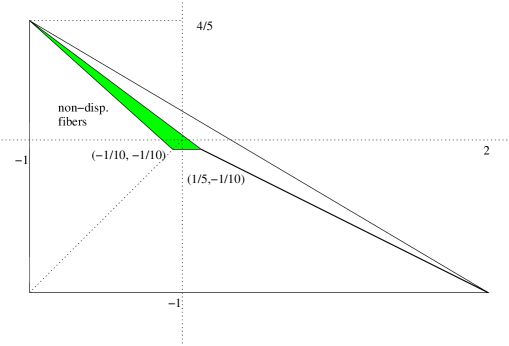
Figure 4. Orbifold $\mathbb{P}(1,3,5)$

As the shape indicates, we need a little detailed analysis on comparing the sizes of the areas of holomorphic discs and orbi-discs.

First we identify elements of $Box^{\prime}$. We find that from $\boldsymbol{b}_{0}$ and $\boldsymbol{b}_{1}$,

$$\nu_{1} =\frac{1}{5}\boldsymbol{b}_{0}+\frac{3}{5}\boldsymbol{b}_{1}= (0,-1)$$

$$\nu_{2} =\frac{2}{5}\boldsymbol{b}_{0}+\frac{1}{5}\boldsymbol{b}_{1}= (-1,-2)$$

$$\nu_{3} =\frac{3}{5}\boldsymbol{b}_{0}+\frac{4}{5}\boldsymbol{b}_{1}= (-1,-3)$$

$$\nu_{4} =\frac{4}{5}\boldsymbol{b}_{0}+\frac{2}{5}\boldsymbol{b}_{1}= (-2,-4)$$

From $\boldsymbol{b}_{0}$ and $\boldsymbol{b}_{2}$, we have

$$\nu_{5} =\frac{1}{3}\boldsymbol{b}_{0}+\frac{2}{3}\boldsymbol{b}_{1}= (-1,-1)$$

$$\nu_{6} =\frac{2}{3}\boldsymbol{b}_{0}+\frac{1}{3}\boldsymbol{b}_{1}= (-2,-3)$$

The areas of holomorphic discs and orbi-discs are

$$\ell_{0}=1-3u_{1}-5u_{2},\;\ell_{1}=1+u_{1},\;\ell_{2}=1+u_{2}$$

$$\ell_{\nu_{1}}=\frac{1}{5}\ell_{0}+\frac{3}{5}\ell_{1}=\frac{4}{5}-u_{2},\;\ell_{\nu_{2}}=\frac{3}{5}-u_{1}-2u_{2}$$

The areas $\ell_{\nu_{3}},\cdots,\ell_{\nu_{6}}$ can be computed similarly.

Near the vertex $(-1,4/5)$ of the moment triangle in Figure 4, the areas of the following (orbi)discs (depending on the position $u\in P$),

$$\ell_{0},\ell_{1},\ell_{\nu_{1}},\ell_{\nu_{2}},\ell_{\nu_{3}},\ell_{\nu_{4}}$$

are smaller than others, and could give relevant terms in the leading term equation.

As it is two dimensional, we would like to have triple of them to have same energy $S_{1}$. Although the symplectic area $\ell_{0},\ell_{1}$ is already fixed, we could add bulk deformation term $\mathfrak{b}_{\nu_{i}}$ to $\ell_{\nu_{i}}$ suitably to increase the energy level. Thus if $\ell_{0}$ is not equal to $\ell_{1}$, we need two other orbi-discs to make the triple, and for this we need them to have smaller symplectic areas.

More precisely, we proceed as follows. First, we consider the region where $\ell_{0}$ or $\ell_{1}$ is smaller than $\ell_{2}$. This implies that

$$\ell_{0}<\ell_{2}\Rightarrow u_{2}>-u_{1}/2,\;\;\;\;\,\ell_{1}<\ell_{2}\Rightarrow u_{2}>u_{1}.$$

We divide it further into three cases:

1. $\ell_{0}<\ell_{1}$, or $u_{1}>-4u_{2}/5$: to have at least three terms of least energy, we need

   $$\ell_{\nu_{1}}<\ell_{0}\;\textrm{and}\;\ell_{\nu_{2}}<\ell_{0}.$$ (15.4)

   The first inequality gives $3u_{1}+4u_{2}<1/5$ and the second inequality gives $2u_{1}+3u_{2}<2/5$. If this happens, we can add bulk deformation

   $$\mathfrak{b}_{\nu_{1}}=T^{\ell_{0}-\ell_{\nu_{1}}},\mathfrak{b}_{\nu_{2}}=T^{\ell_{0}-\ell_{\nu_{2}}}.$$

   which will make $\boldsymbol{b}_{0},\boldsymbol{b}_{\nu_{1}},\boldsymbol{b}_{\nu_{2}}$ to contribute to the leading term equation of $PO^{\mathfrak{b}}_{orb,0}$ of the same energy $S_{1}$. We note that the first inequality implies the second inequality for the points in $P$, hence, for the region bounded by

   $$u_{1}>-\frac{4u_{2}}{5},\;\;3u_{1}+4u_{2}<\frac{1}{5},\;\;u_{2}>-\frac{u_{1}}{2},$$

   we can choose bulk deformation as above, so that the corresponding leading term equation has a solution.

2. $\ell_{0}>\ell_{1}$ or $u_{1}<-4u_{2}/5$: to have at least three terms of least energy, we need

   $$\ell_{\nu_{1}}<\ell_{1}\;\textrm{and}\;\ell_{\nu_{2}}<\ell_{1}.$$ (15.5)

   Both equation translates to the inequality $u_{1}+u_{2}>-1/5$. Thus, in the region

   $$u_{1}<-\frac{4u_{2}}{5},\;\;\;u_{1}+u_{2}>\mathfrak{1}{5},\;\;\;u_{2}>u_{1},$$

   we can choose bulk deformation as

   $$\mathfrak{b}_{\nu_{1}}=T^{\ell_{1}-\ell_{\nu_{1}}},\mathfrak{b}_{\nu_{2}}=T^{\ell_{1}-\ell_{\nu_{2}}},$$

   so that the corresponding leading term equation has a solution.

3. $\ell_{0}=\ell_{1}$: similarly, we obtain that the line segment $u_{1}=-\frac{4u_{2}}{5},u_{1}<0$ supports bulk deformation, whose leading term equation has a solution, which we leave as an exercise.

The above do not cover the whole colored region of the Figure 4. The rest of the region, which is not covered is the triangle $\Delta$ formed by three points

$$(-1/10,-1/10),(0,0),(1/5,-1/10).$$

For this region, the leading term equation involves two equations of two energy level $S_{1}$, $S_{2}$. Note that the vectors $\boldsymbol{b}_{2}=(0,1)$ and $\boldsymbol{b}_{\nu_{1}}=(0,-1)$ are opposite to each other. So in $\Delta$, $\ell_{2}$ is smaller than $\ell_{1}$ and $\ell_{0}$, and hence we take

$$\mathfrak{b}_{\nu_{1}}=T^{\ell_{2}-\ell_{\nu_{1}}}=T^{2u_{2}+\frac{1}{5}}.$$

This makes the terms corresponding to $\boldsymbol{b}_{1}$ and $\boldsymbol{b}_{\nu_{1}}$ contribute to the leading term equation of energy level $S_{1}=\ell_{2}$. Now, for the next level $S_{2}$, we have terms from $\boldsymbol{b}_{1}$, and $\boldsymbol{b}_{\nu_{2}}$, we again have a solution for $S_{2}$ energy level leading term equation. We leave the detailed check tot he readers.

We remark that for the line segment from $(1/5,-1/10)$ to $(2,-1)$, it is known by [WW] to be non-displaceable, but our methods cannot prove it yet as in Remark15.1.

15.6. Polytope with nontrivial integer labels

Proposition 15.2.

If $P$ is compact rational simple polytope with $m$ facets, and if the integer labels, $c_{1},\cdots,c_{m}$ for facets satisfy

$$c_{i}\geq 2\;\;\textrm{for all}\;\;i=1,\cdots,m,$$

then for any $u\in Int(P)$, $L(u)$ is non-displaceable.

Proof.

The first proof is due to Kaoru Ono, who have provided this alternative proof after the first authors gave a talk on this paper and this proposition.

Here is the first proof. As all facets have non-trivial integer labels, points in any toric divisors are not smooth points. Take a torus fiber $L(u)$ for any interior point $u\in Int(P)$. If $L(u)$ is displaceable by Hamiltonian isotopy $\psi^{H}_{1}$, i.e. $L(u)\cap\psi^{H}_{1}(L(u))=\emptyset$, then we can modify $H$ so that its support lies in $Int(P)$, and satisfy the above displacing property as Hamiltonian isotopy sends smooth points to smooth points. But this is a contradiction, since Lagrangian torus fibers in $(\mathbb{C}^{*})^{n}$ are not displaceable by any compactly supported Hamiltonian isotopy. As a symplectic manifold, the inverse image $L$ of $Int(P)$ is symplectically embedded in $T^{*}T^{n}$. Then a $T^{n}$-orbit is considered as the graph of a $T^{n}$-invariant $1$-form $\eta$ on $T^{n}$, which is closed, embedded in $T^{*}T^{n}$. By a symplectomorphism, which comes from the fiberwise addition of $-\eta$, we may assume that the $T^{n}$-orbit is the zero section of $T^{*}T^{n}$. The non-displaceability of the zero section in the cotangent bundle is a well-known.

The second proof is by using the bulk deformation. Let $\boldsymbol{b}_{i}$ be a stacky vector corresponding to the $i$-th facet. We take $\nu_{i}$ to be the minimal integral vector in the direction of $\boldsymbol{b}_{i}$ such that $\boldsymbol{b}_{i}=c_{i}\nu_{i}$. We consider bulk deformations $\mathfrak{b}_{\nu_{i}}=-c_{i}T^{\ell_{i}-\ell_{\nu_{i}}}$ for each $i=1,\cdots,m$. Then corresponding leading term potential $PO^{\mathfrak{b}}_{orb,0}$ becomes

$$\sum_{i=1}^{m}T^{\ell_{i}}(y^{\boldsymbol{b}_{i}}-c_{i}y^{\boldsymbol{b}_{\nu_{i}}}),$$ (15.6)

since each contribution of $\mathfrak{b}_{\nu_{i}}$ is chosen to match with the term of the potential corresponding to $\boldsymbol{b}_{i}$. For generic $u$, we may assume that all the areas $\ell_{i}$ are distinct. Then, the leading term equation is the critical point equation of each summand of 15.6 up to dimension of $P$. By denoting $y_{l}=y^{\boldsymbol{b}_{\nu_{i}}}$, the summand equals $y_{l}^{c_{i}}-c_{i}y_{l}$, and clearly has a non-trivial critical point $y_{l}=1$. This shows that generic $u\in Int(P)$ is non-displaceable. But by the standard limit argument, this implies that $L(u)$ is non-displaceable for all $u\in Int(P)$. ∎

16. Appendix: Preliminaries on orbifold maps

In this appendix, we recall definitions regarding maps between orbifolds following [CR], [CR2] with the condition that the domain orbifold may have a nontrivial smooth boundary.

Let ${\mathcal{X}}$ be a differentiable ($C^{\infty}$) orbifold with boundary and let $X$ be its underlying topological space. In applications we will often deal with the case when $X$ is an orbifold Riemann surface with smooth boundary (i.e. orbifold singularity lies in the interior).

An uniformizing system for an open connected set $U\subset X$ is a triple $(V,G,\pi)$ where $V$ is a smooth connected manifold with boundary $\partial V$ (which may be empty), $G$ is a finite group acting smoothly on $V$ (preserving $\partial V$) , and $\pi:V\to U$ is a continuous map that induces a homeomorphism between $V/G$ and $U$. The orbifold analogue of inclusion of open sets in manifolds, is the notion of injection of uniformizing charts.

Definition 16.1.

Let $i:U\hookrightarrow U^{\prime}$ be an inclusion of open sets uniformized by $(V,G,\pi)$ and $(V^{\prime},G^{\prime},\pi^{\prime})$ respectively. An injection $(\phi,\rho):(V,G,\pi)\to(V^{\prime},G^{\prime},\pi^{\prime})$ consists of an injective group homomorphism $\rho:G\to G^{\prime}$ and a $\rho$-equivariant open embedding $\phi:V\to V^{\prime}$ such that

1. $i\circ\pi=\pi^{\prime}\circ\phi$ and

2. $\rho$ induces an isomorphism $\ker G\to\ker G^{\prime}$ where $\ker G:=\{g\in G:g\cdot x=x\;{\rm for\;all\;}x\in V\}$.

If $\ker G$ is trivial for every uniformizing system, the orbifold is called effective or reduced.

An injection $(\phi,\rho)$ is an isomorphism of uniformizing systems if there exists an inverse injection. An important fact is that given an automorphism $(\phi,\rho)$ of an uniformizing system $(V,G,\pi)$ of open set $U\subset X$ in a $C^{\infty}$ orbifold ${\mathcal{X}}$ (with boundary), there exists an element $g\in G$ such that $\phi(x)=gx$ and $\rho(h)=ghg^{-1}$, see Lemma 2.11 of [MM]. This correspondence is one-to-one if $\ker G$ is trivial.

Definition 16.2.

A compatible cover of an open set $Y$ in an orbifold ${\mathcal{X}}$ is an open cover $\mathcal{U}$ of $Y$ together with an uniformizing system $(V,G,\pi)$ for each $U\in\mathcal{U}$ and a collection of injections such that

1. If $U\subset U^{\prime}$ then there exists an injection $(V,G,\pi)\to(V^{\prime},G^{\prime},\pi^{\prime})$.

2. For every $p\in U_{1}\bigcap U_{2}$, where $U_{1},U_{2}\in\mathcal{U}$, there exists an $U\in\mathcal{U}$ such that $p\in U\subset U_{1}\bigcap U_{2}$.

Definition 16.3.

Let ${\mathcal{X}}$ and ${\mathcal{X}}^{\prime}$ be orbifolds, possibly with boundary. Suppose $U\subset X,\,U^{\prime}\subset X^{\prime}$ are open sets uniformized by $(V,G,\pi)$ and $(V^{\prime},G^{\prime},\pi^{\prime})$ respectively. Given a continuous map $f:U\to U^{\prime}$, a $C^{l}$ lift of $f$ is a $C^{l}$ map $\tilde{f}:V\to V^{\prime}$ satisfying

1. $\pi^{\prime}\circ\tilde{f}=f\circ\pi$.

2. Given any $g\in G$ there exists a $g^{\prime}\in G^{\prime}$ such that $\tilde{f}(gx)=g^{\prime}\tilde{f}(x)$ for all $x\in V$.

Note that the correspondence $g\to g^{\prime}$ is not required to be a group homomorphism.

Definition 16.4.

Two lifts $\tilde{f}_{i}:(V_{i},G_{i},\pi_{i})\to(V_{i}^{\prime},G_{i}^{\prime},\pi_{i}^{\prime})$, $i=1,2$, are isomorphic if there are isomorphisms $(\phi,\rho):(V_{1},G_{1},\pi_{1})\to(V_{2},G_{2},\pi_{2})$ and $(\phi^{\prime},\rho^{\prime}):(V_{1}^{\prime},G_{1}^{\prime},\pi_{1}^{\prime})\to(V_{2}^{\prime},G_{2}^{\prime},\pi_{2}^{\prime})$ such that $\phi^{\prime}\circ\tilde{f}_{1}=\tilde{f}_{2}\circ\phi$.

Let $\tilde{f}:(V,G,\pi)\to(V^{\prime},G^{\prime},\pi^{\prime})$ be a $C^{l}$ lift of $f:U\to U^{\prime}$. Let $W,\,W^{\prime}$ be open sets such that $W\subset U$ and $f(W)\subset W^{\prime}\subset U^{\prime}$. Then $\tilde{f}$ naturally induces a unique isomorphism class of lift for $f:W\to W^{\prime}$.

Definition 16.5.

Two lifts $\tilde{f}_{i}:(V_{i},G_{i},\pi_{i})\to(V_{i}^{\prime},G_{i}^{\prime},\pi_{i}^{\prime})$, $i=1,2$, of $f:X\to X^{\prime}$ over open sets $U_{1}$ and $U_{2}$, are said to be equivalent at $p\in U_{1}\bigcap U_{2}$ if they induce isomorphic lifts of $f:U\to U^{\prime}$ for some open sets $U$ containing $p$ and $U^{\prime}$ containing $f(p)$.

Definition 16.6.

A local $C^{l}$ lift of $f:X\to X^{\prime}$ at a point $p\in X$ is a $C^{l}$ lift $\tilde{f}_{p}:V_{p}\to V_{f(p)}^{\prime}$, for some uniformizing systems $(V_{p},G_{p},\pi_{p})$ and $(V_{f(p)}^{\prime},G^{\prime}_{f(p)},\pi^{\prime}_{f(p)})$ on open sets containing $p$ and $f(p)$ respectively.

Definition 16.7.

Let ${\mathcal{X}}$ and ${\mathcal{X}}^{\prime}$ be orbifolds, possibly with boundary. Given a continuous map $f:X\to X^{\prime}$, a $C^{l}$ lift ${\tilde{f}}:{\mathcal{X}}\to{\mathcal{X}}^{\prime}$ of $f$ is a choice of a local $C^{l}$ lift $\tilde{f}_{p}:V_{p}\to V_{f(p)}^{\prime}$ for each point $p$, such that $\tilde{f}_{p}$ is equivalent to $\tilde{f}_{q}$ for each $q\in U_{p}$.

Example 16.8.

Consider the orbifold $\mathbb{C}/\mathbb{Z}_{2}$ where $\mathbb{Z}_{2}$ acts by reflection about the origin. Consider the holomorphic coordinates $z$ on $\mathbb{C}$ and $w=z^{2}$ on $\mathbb{C}/\mathbb{Z}_{2}$. Regard $S^{1}$ as $\mathbb{R}/2\pi\mathbb{Z}$. Take the map $f:S^{1}\to\mathbb{C}/\mathbb{Z}_{2}$ defined by $w\circ f(\theta)=e^{i\theta}$. Consider the covering of $S^{1}$ by the open sets $U_{1}=(0,2\pi)$ and $U_{2}=(-\pi,\pi)$. The lifts $\tilde{f}_{j}:U_{j}\to\mathbb{C}$ given by

$$z\circ\tilde{f}_{j}(\theta)=e^{i\theta/2}\;{\rm for\,}j=1,2,$$ (16.1)

define a $C^{\infty}$ lift of $f$.

Note that not every continuous map of underlying spaces admits a lift. As an example, the map $h:\mathbb{C}\to\mathbb{C}/\mathbb{Z}_{2}$ defined by $w\circ h(t)=t$, does not admit even a $C^{0}$ lift near the origin.

Definition 16.9.

Two lifts $\{\tilde{f}_{p,i}:(V_{p,i},G_{p,i},\pi_{p,i})\to(V_{f(p),i}^{\prime},G^{\prime}_{p,i},\pi^{\prime}_{f(p),i})\},\;i=1,2,$ of $f$ are said to be equivalent if for each $p\in X$, $\tilde{f}_{p,1}$ and $\tilde{f}_{p,2}$ are equivalent at $p$.

Definition 16.10.

A $C^{l}$ map of orbifolds ${\bf f}:{\mathcal{X}}\to{\mathcal{X}}^{\prime}$ is a continuous map $f:X\to X^{\prime}$ of underlying spaces together with the equivalence class of a $C^{l}$ lift $\tilde{f}$ of $f$.

Now we recall the crucial notion of a good map[CR]. Chen and Ruan used the notion of compatible system to describe a good map. A compatible system roughly consists of compatible covers of the domain and range of the map by uniformizing charts, choice of lifts on each chart and some algebraic data for injections of charts that encode how the lifts fit together. This enables one to define the pull-back of an orbifold vector bundle with respect to a good map. The notion of good map is very closely related to the notions of strong map [MP] and orbifold morphism [ALR].

Definition 16.11.

Let ${\bf f}:{\mathcal{X}}\to{\mathcal{X}}^{\prime}$ be a $C^{l}$ map between orbifolds with boundary whose underlying continuous map is denoted by $f$. Suppose $\mathcal{U}$ and $\mathcal{U}^{\prime}$ are compatible covers of $X$ and an open set containing $f(X)$ respectively satisfying the following conditions

1. There is a bijection between $\mathcal{U}$ and $\mathcal{U}^{\prime}$ given by $U\leftrightarrow U^{\prime}$, such that $f(U)\subset U^{\prime}$, and $U_{2}\subset U_{1}$ implies $U_{2}^{\prime}\subset U_{1}^{\prime}$.

2. There exists a collection of local $C^{l}$ lifts $\{\tilde{f}_{UU^{\prime}}:(V,G,\pi)\to(V^{\prime},G^{\prime},\pi^{\prime})\}$ of $f$ and an assignment of an injection $\lambda(i):(V_{2}^{\prime},G_{2}^{\prime},\pi_{2}^{\prime})\to(V_{1}^{\prime},G_{1}^{\prime},\pi_{1}^{\prime})$ to every injection $i:(V_{2},G_{2},\pi_{2})\to(V_{1},G_{1},\pi_{1})$ such that

   1. $\tilde{f}_{U_{1}U_{1}^{\prime}}\circ i=\lambda(i)\circ\tilde{f}_{U_{2}U_{2}^{\prime}}$

   2. $\lambda(j\circ i)=\lambda(j)\circ\lambda(i)$ for each composition $j\circ i$ of injections.

3. The $C^{l}$ lift of $f$ defined by the collection $\{\tilde{f}_{UU^{\prime}}\}$ is in the equivalence class corresponding to $\bf f$.

Then we say that $\{\tilde{f}_{UU^{\prime}},\lambda\}$ is a compatible system of ${\bf f}$.

Note that if ${\mathcal{X}}^{\prime}$ is reduced, each automorphism $g\in G$ of $(V,G,\pi)$ is assigned an automorphism $\lambda(g)\in G^{\prime}$ giving rise, by condition (2)(b), to a group homomorphism $\lambda_{UU^{\prime}}:G\to G^{\prime}$ with respect to which $\tilde{f}_{UU^{\prime}}$ is equivariant.

Definition 16.12.

A $C^{l}$ map ${\bf f}:{\mathcal{X}}\to{\mathcal{X}}^{\prime}$ is called a good $C^{l}$ map if it admits a compatible system.

When an orbifold is reduced, it may be represented as the quotient of a manifold by the effective action of a compact Lie group by the so-called frame bundle trick. However a good map between ${\mathcal{X}}=M/G$ and ${\mathcal{X}}^{\prime}=N/H$ may not be represented by an equivariant map from $M$ to $N$. This has to do with the fineness of the compatible cover of ${\mathcal{X}}$ used to define the good map. Indeed, a similar problem occurs for a good map from a manifold to an orbifold. For instance consider the $C^{\infty}$ map $S^{1}\to\mathbb{C}/\mathbb{Z}_{p}$ given by the lift $t\mapsto t^{1/p}$. We need to use a suitable cover of $S^{1}$ to make sense of continuity of the lift.

A good $C^{\infty}$ map is what Chen and Ruan[CR] calls a good map. Not all orbifold maps admit a compatible system. See example 4.4.2a of [CR].

Chen and Ruan prove (cf. Lemma 4.4.6 and Remark 4.4.7 of [CR]) that given two compatible systems $\xi_{1}=\{\tilde{f}_{1,UU^{\prime}},\alpha_{1}:U\in\mathcal{U},U^{\prime}\in\mathcal{U^{\prime}}\}$, and $\xi_{2}=\{\tilde{f}_{2,RR^{\prime}},\alpha_{2}:R\in\mathcal{R},R^{\prime}\in\mathcal{R^{\prime}}\}$ for a $C^{\infty}$ map ${\bf f}:{\mathcal{X}}\to{\mathcal{X}}^{\prime}$, there exist

1. common refinements $\mathcal{W}$ of $\mathcal{U}$ and $\mathcal{R}$, and $\mathcal{W}^{\prime}$ of $\mathcal{U}^{\prime}$ and $\mathcal{R}^{\prime}$, that satisfy condition(1) of definition 16.11,

2. compatible systems $\{\tilde{f}_{1,WW^{\prime}},\lambda_{1}\}$ and $\{\tilde{f}_{2,WW^{\prime}},\lambda_{2}\}$, where $W\in\mathcal{W}$ and $W^{\prime}\in\mathcal{W}^{\prime}$, for ${\bf f}$ induced by $\xi_{1}$ and $\xi_{2}$ respectively.

Chen-Ruan’s proof actually works for any $C^{l}$ map where $l\geq 0$. An important consequence of Lemma 4.4.6 of [CR] is that the compatible systems $\{\tilde{f}_{i,WW^{\prime}},\lambda_{i}\}$ can be assumed to be geodesic compatible systems (see Definition 4.4.5 of [CR]). In particular, the open sets of $\mathcal{W}$ and $\mathcal{W}^{\prime}$ are images of the exponential map from some subset of the tangent space at some point in their interiors. This property is crucial to relate compatible systems with pull-back of vector bundles, especially the tangent bundle. This will continue to hold if ${\mathcal{X}}$ is an orbifold Riemann surface with smooth boundary, for appropriate choice of Riemannian metric on ${\mathcal{X}}$. (The idea is to choose a Riemannian metric on the double ${\mathcal{Y}}$ of ${\mathcal{X}}$ that agrees with a metric on the manifold $Y$ away from a small neighborhood of the singular set. Then use the positivity of the injective radius of the metric on $Y$.)

The following definition is equivalent to, but different from, the one in [CR].

Definition 16.13.

Two compatible systems $\xi_{1}$ and $\xi_{2}$ of a good $C^{l}$ map ${\bf f}$ are said to be isomorphic if there exist induced compatible systems $\{\tilde{f}_{1,WW^{\prime}},\lambda_{1}\}$ and $\{\tilde{f}_{2,WW^{\prime}},\lambda_{2}\}$ corresponding to $\xi_{1}$ and $\xi_{2}$ respectively, and an automorphism $\delta_{V^{\prime}}$ of the uniformizing system $(V^{\prime},G^{\prime},\pi^{\prime})$ for each $W^{\prime}\in\mathcal{W}^{\prime}$, such that

1. $\delta_{V^{\prime}}\circ\tilde{f}_{1,WW^{\prime}}=\tilde{f}_{2,WW^{\prime}}$ and

2. for each injection $i:(W_{2},G_{2},\pi_{2})\to(W_{1},G_{1},\pi_{1})$, the relation $\lambda_{2}(i)=\delta_{V_{1}^{\prime}}\circ\lambda_{1}(i)\circ(\delta_{V_{2}^{\prime}})^{-1}$ holds.

The proof of the following lemma is similar to Proposition 4.4.8 of [CR].

Lemma 16.1.

Suppose ${\bf f}:{\mathcal{X}}\to{\mathcal{X}}^{\prime}$ is a good $C^{\infty}$ map where ${\mathcal{X}}$ is an orbifold with smooth boundary. Then two compatible systems $\xi_{1}$ and $\xi_{2}$ are isomorphic if and only if the pullbacks of any orbifold vector bundle on ${\mathcal{X}}^{\prime}$ by $\xi_{1}$ and $\xi_{2}$ are isomorphic.

References

• [ABM] M. Abreu, M. S. Borman and D. McDuff Displacing Lagrangian toric fibers by extended probes, arXiv:1203.1074.
• [AM] M. Abreu, L. Macarini. Remarks on Lagrangian intersections on toric manifolds. To appear in Trans. Am. Math. Soc. arXiv:1105.0640.
• [ALR] A. Adem, J. Leida and Y. Ruan, Orbifolds and stringy topology, Cambridge Tracts in Mathematics 171, Cambridge University Press, Cambridge, 2007.
• [Ar] Arnolโ€™d, V. I. On a characteristic class entering the quantization conditions, Funct. Anal. Appl. 1,1967, pp. 1-14
• [Au] M. Audin, The Topology of Torus Actions on Symplectic Manifolds, Birkhรคuser Verlag, Basel, Progress in Mathematics 93, 1991.
• [B1] V. Batyrev, Quamtum cohomology rings of toric manifolds, Journees de geometrie Algebrique dโ€™Orsay, 1992, Asterisque 218, 9-34.
• [BCS] L. Borisov, L. Chen, G. Smith The orbifold Chow ring of toric Deligne-Mumford stacks. J. Amer. Math. Soc. 18 (2005), no. 1, 193โ€“215
• [C1] C.-H. Cho Holomorphic discs, spin structures and the Floer cohomology of the Clifford torus, IMRN (2004) no. 35 1803-1843
• [C2] C.-H. Cho Products of Floer cohomology of Lagrangian torus fibers in toric Fano manifolds Commun. Math. Phy. 260, 613-640 (2005)
• [C3] C.-H. Cho Non-displaceable Lagrangian submanifolds and Floer cohomology with non-unitary line bundle, J. Geom. Phys. 58 (2008), 1465-1476
• [CO] C.-H. Cho, Y.-G. Oh Floer cohomology and disc instantons of Lagrangian torus fibers in toric Fano manifolds Asian Journ. Math. 10 (2006), 773-814
• [CR] W. Chen, Y. Ruan Orbifold Gromov-Witten invariants, Orbifolds in mathematics and physics, Contemporary mathematics 310 (210), 25โ€“85, 2002
• [CR2] W. Chen, Y. Ruan A new cohomology theory of orbifolds, Comm. Math. Phys. 248:1 1โ€“31, 2004
• [CS] C.-H. Cho, H.-S. Shin Maslov index via Chern-Weil theory and an orbifold analouge, arXiv:1202.0556
• [Co] D. Cox, Homogeneous coordinate ring of a toric variety, J. algebraic Geometry 4 (1995), 17-50.
• [Fl] A. Floer, Morse theory for Lagrangian intersections, J. Differ. Geom. 28 (1988), 513-547.
• [FO] K. Fukaya, K. Ono Arnold conjecture and Gromov-Witten invariants, Topology 38 (1999), 933โ€“1048.
• [FOOO] K. Fukaya, Y.-G. Oh, H. Ohta and K. Ono, Lagrangian intersection Floer theory-anomaly and obstruction, Part I, II, AMS/IP Studies in Adv. Math, 46.1. AMS, International Press, 2009.
• [FOOO2] K. Fukaya, Y.-G. Oh, H. Ohta and K. Ono, Lagrangian Floer theory for toric manifolds I Duke Math. Journ. vol.151, no.1,2009
• [FOOO3] K. Fukaya, Y.-G. Oh, H. Ohta and K. Ono, Lagrangian Floer theory for toric manifolds II: Bulk deformations, Selecta Math, New Series, Volume 17, Number 3 (2011), 609-711
• [FOOO4] K. Fukaya, Y.-G. Oh, H. Ohta and K. Ono, Lagrangian Floer theory and mirror symmetry on compact toric manifolds, arXiv:1009.1648
• [FOOO5] K. Fukaya, Y.-G. Oh, H. Ohta and K. Ono, Lagrangian Floer theory on compact toric manifolds:Survey arXiv:1011.4044
• [FOn] K. Fukaya and K. Ono, Arnold conjecture and Gromov-Witten invariants, Topology 38 (1999), 933-1048.
• [Ful] W. Fulton, Introduction to Toric Varieties, Annals of Mathematics Studies, 131, Princeton University Press, Princeton, 1993.
• [HV] K. Hori and C. Vafa, Mirror Symmetry, arXiv:hep-th/0002222v3
• [Ki] F. Kirwan, Cohomology of quotients in symplectic and algebraic geometry, Math. notes 31, Princeton Univ. Press
• [KL] S. Katz and C.C. Liu, Enumerative geometry of stable maps with Lagrangian boundary conditions and multiple covers of the disc, Adv. Theor. Math. Phys. 5 (2001), 1-49.
• [Ko] M. Kontsevich, Homological algebra of mirror symmetry, ICM-1994 Proceedings, Zรผrich, Birkhรคuser, 1995.
• [LT] E. Lerman, S. Tolman Hamiltonian torus actions on symplectic orbifolds and toric varieties. Trans. Amer. Math. Soc., 349(10):4201โ€šร„รถโˆšร‘โˆšยจ4230, 1997
• [M] D. McDuff Displacing Lagrangian toric fibers via probes. Low-dimensional and symplectic topology, 131-160, Proc. Sympos. Pure Math., 82, Amer. Math. Soc., Providence, RI, 2011.
• [MP] I. Moerdijk and D. A. Pronk, Orbifolds, sheaves and groupoids, K-theory 12:1 (1997), 3-21.
• [MM] I. Mooerdijk and J. Mr$\check{\rm c}$un, Introduction to foliations and Lie groupoids, Cambridge Studies in Advanced Mathematics, Cambridge University Press, Cambridge, 2003.
• [MW] J. Marsden and A. Weinstein, Reduction of symplectic manifolds with symmetry, Reports on Math. Phys. 5 (1974), 121-130.
• [O1] Y.-G. Oh, Floer cohomology of Lagrangian intersections and pseudo-holomorphic discs I, Comm. Pure and Appl. Math. 46 (1993), 949-994 addenda, ibid, 48 (1995), 1299-1302.
• [O2] Y.-G. Oh, Floer cohomology of Lagrangian intersections and pseudo-holomorphic discs II & III, Comm. Pure Appl. Math. 46 (1993), 995-1012 & The Floer Memorial Volume (ed. by H. Hofer et al.), Birkhรคuser, Basel, pp 555-573, 1995.
• [Wh] G. W. Whitehead, Elements of Homotopy Theory, Graduate Texts in Mathematics, 61. Springer-Verlag, New York-Berlin, 1978.
• [WW] G. Wilson, C. Woodward, Quasimap Floer cohomology and varying symplectic quotients, arXiv:1105.0712
• [Wo] C. Woodward, Gauged Floer theory of toric moment fibers, arXiv: 1004.2841