Scattering of quasi-one-dimensional solitons on impurities in large Josephson junctions

Abstract

Fluxon transmission through impurities of different shape in a quasi-one-dimensional long Josephson junction is investigated. The junction width is significantly less than its length but, at the same time, is of the order of the Josephson penetration length $\lambda_{J}$ or exceeds it. The retrapping current on the impurities of the point, line and rectangular shape is computed as a function of the junction width both numerically and analytically. Good agreement between the analytic formulae and the numerical simulation results for the intermediate (several $\lambda_{J}$) junction width is observed.

1 Introduction

The dynamics of magnetic flux propagation in a long Josephson junction (LJJ) has been and continues to be a subject of strong theoretical and practical interest during the last three decades [1, 2, 3]. The magnetic flux quantum in a LJJ is a soliton (also known as fluxon) governed by the well-known sine-Gordon (SG) equation. The convenient way to prepare a junction with the required properties is to install various inhomogeneities into it. Up to now the substantial theoretical work has been devoted to the study of the fluxon motion in the one-dimensional (1D) LJJs with point-like [4, 5, 6] and spatially extended [7, 8, 9] inhomogeneities. Experimental results on the fluxon scattering on impurities are reported in [6, 10] Spatially inhomogeneous Josephson systems with trapped fluxons have been discussed as prospective applications, such as fluxon-based information devices [11, 12].

Real LJJs are always two-dimensional (2D), or, more precisely, quasi-one-dimensional (Q1D), in the sense that they have a finite width in the direction perpendicular to the direction of fluxon propagation. Up to now the fluxon dynamics in Q1D junctions has been scarcely investigated as compared to the pure 1D case. Most of attention has been focused on the various isotropic 2D structures like oscillons and ring kinks [13]. It is worth mentioning also the case of window junctions [14, 15], which can be called inverse in some sense: it studies point or rectangular junctions embedded in a larger two-dimensional superconduncting sample. Quasi-one-dimensional solitons, or, in other words, solitonic fronts in infinite (in both $x$ and $y$ directions) samples have been studied in detail by Malomed [16]. Several interesting results in the absence of dissipation have been reported including the waves in the Q1D sine-Gordon equation, travelling along the soliton line [17] and skyrmion scattering on impurities in the 2D baby Scyrme model [18]. However, in the case of the fluxon dynamics in a LJJ the presence of dissipation is unavoidable.

It is of interest to investigate the Q1D fluxon dynamics in the presence of spatial inhomogeneities when the junction width is finite. We expect that the fluxon transmission in this case will be significantly enhanced comparing to the pure 1D case. For example, in the previously studied case of the lattice acoustic soliton front interaction with mass impurities [19] it has been shown that the front can round the point impurity while a 1D lattice soliton gets reflected from it. Moreover, the soliton front can overcome even the impurity of the infinite mass. To our knowledge the fluxon interaction with spatial inhomogeneities has not been studied except in [16], however this paper deals only with the infinite sample width.

Thus, in this Letter we aim at studying the Q1D fluxon interaction with impurities and finding out how this interaction depends on the junction width and other system parameters. In particular, it is planned to find how the retrapping current (e.g., the minimal bias current for which the fluxon propagation is still possible) depends on the junction width.

The paper is organized as follows. In the next section, the model is described. Section 3 is devoted to the fluxon transmission through impurities. In the last section discussion and conclusions are presented.

2 The model

We consider the Q1D long Josephson junction (LJJ) subjected to the external time-independent bias. The main dynamical variable is the difference between the phases $\theta_{2}(x,y;t)-\theta_{1}(x,y;t)=\phi(x,y;t)$ of the macroscopic wave functions of the superconducting layers of the junction. The time evolution of the phase difference is governed by the perturbed sine-Gordon (SG) equation of the form

$$\phi_{tt}-\Delta\phi+[1+f(x,y)]\sin\phi=-\alpha\phi_{t}-\gamma,$$ (1)

where $\Delta\phi=\phi_{xx}+\phi_{yy}$ and the indexes ${t,x,y}$ stand for the respective partial derivatives. In this dimensionless equation the spatial variables $x$ and $y$ are normalised to the Josephson penetration depth $\lambda_{J}$, the temporal variable $t$ is normalised to the inverse Josephson plasma frequency $\omega_{J}^{-1}$ [1, 2]. The bias current $\gamma$ is normalised to the critical Josephson current of the junction and $\alpha$ is the dimensionless dissipation parameter. The function $f(x,y)$ describes the spatial inhomogenity. In the case of point impurities in the general form it reads

$$f(x,y)=\sum_{n=1}^{N}\mu\delta(x-a_{n})\delta(y-b_{n})\>.$$ (2)

It is supposed that there are $N$ impurities in this junction, positioned at the points $x=a_{n}$, $y=b_{n}$, $n=1,2,\ldots,N$, with $\mu$ being the “strength” or the amplitude of the impurity. Only the microshorts ($\mu>0$), i.e., a narrow regions of locally enhanced critical density of the tunnelling superconctucting current will be investigated in this article. However, the size an inhomogeneity in experimental samples is finite [10]. Therefore, we consider also the case of the line microshort of width $d_{y}$, stretched along the $y$ direction:

$$f(x,y)=\mu\delta(x)\left[\theta\left(y+\frac{d_{y}}{2}\right)+\theta\left(\frac{d_{y}}{2}-y\right)\right]\,.$$ (3)

Here $\theta(x)$ is the Heavyside function. And finally, the rectangular impurity of the finite size in both $x$ and $y$ directions

$$f(x,y)={\mu}\left[\theta\left(x+\frac{d_{x}}{2}\right)+\theta\left(\frac{d_{x}}{2}-x\right)\right]\left[\theta\left(y+\frac{d_{y}}{2}\right)+\theta\left(\frac{d_{y}}{2}-y\right)\right]$$ (4)

will be considered as well. It should be noted that the impurity strength $\mu$ has different meanings in all three cases (2)-(4). For the point impurity (2) setting $w=0$ does not automatically yield the pure 1D case studied before in [4, 5, 6]. This case can be retained in the strip impurity case if $d_{y}=w$. The 1D finite-size impurity case [7, 8, 9] is retained in the same way.

We choose the boundary conditions along the $y$ direction in the von Neumann form:

$$\phi_{y}\left(x,-{w\over 2},t\right)=\phi_{y}\left(x,{w\over 2},t\right)=0.$$ (5)

The boundary conditions along the $x$ axis are periodic: $\phi(x+L,y;t)=\phi(x,y;t)+2\pi$, where $L$ is the junction length, $L>w\gg 1$.

3 Quasi-one-dimensional fluxon transmission through an impurity

3.1 Numerical simulations

In order to get an idea about the character of the fluxon dynamics, the numerical integration of the Q1D SG equation (1) has been performed. The Josephson phase and its space derivatives are discretized in the following way: $\phi(x,y;t)\to\phi(mh,nh;t)\equiv\phi_{mn}(t)$,
$\Delta\phi\simeq h^{-2}\left(\phi_{m+1,n}+\phi_{m,n+1}+\phi_{m-1,n}+\phi_{m,n-1}-4\phi_{mn}\right)$, while the $\delta$-function is approximated by the Kronecker $\delta$-symbol. The resulting set of ODE’s with the boundary conditions were integrated using the 4th order Runge-Kutta scheme. Details of the fluxon propagation through the two identical point impurities (2) placed along the $y$ axis at $a_{1}=a_{2}=0$ and $b_{1}=-b_{2}=2$ are given in Fig. 1. It is important to mention that the dissipation in Eq. (1) is crucial and the soliton interaction with impurities differs from the dissipationless case where the complex resonant behaviour occurs either for the $\delta$-like [20] or for the finite-size [21] obstacles. Far away from the impurities the fluxon exists as only one attractor of the system with the velocity, predefined by the damping parameter and external bias. Therefore, contrary to the non-dissipative case, the transmission consists of only two possible scenarios: trapping and passage.

For the sake of better visualization the derivative $-\phi_{t}$ is plotted on the $xy$ plane for the different time moments and for three different dissipation values: $\alpha=0.1$, $\alpha=0.05$ and $\alpha=0.01$. Without loss of generality the topological charge is assumed to be $Q=1$ (soliton) throughout the paper. The initial conditions are taken in the form of the approximate (invariant in the $y$ direction) soliton solution, placed at the beginning of the junction and having with the equilibrium velocity.

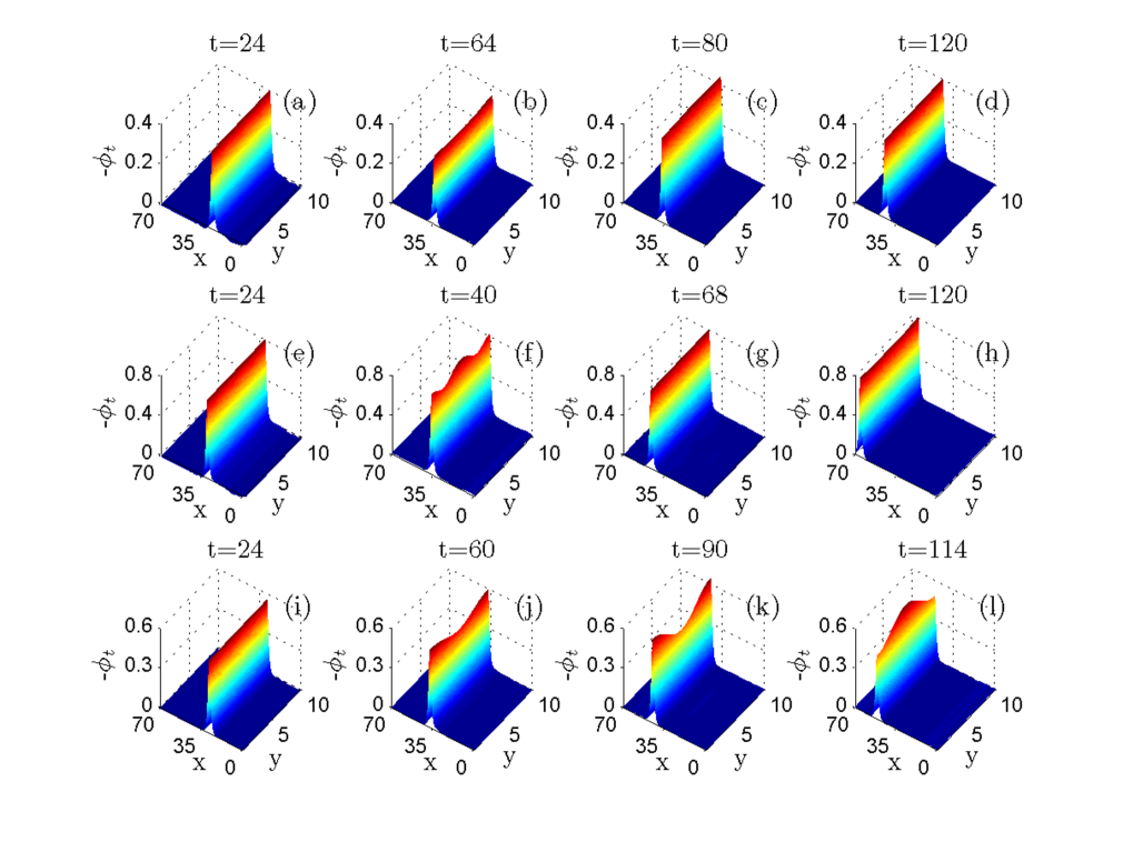
Figure 1: (Colour online) Time evolution of the Josephson phase derivative in the $L=70\times w=10$ junction with $N=2$ impurities with the distance $a_{y}=4$ between them at $\mu=0.5$ and $\alpha=0.1$, $\gamma=0.03$ [(a)-(d)], $\alpha=0.05$, $\gamma=0.02$ [(e)-(h)], $\alpha=0.01$, $\gamma=0.0035$ [(i)-(l)].

The fluxon interaction with the rectangular impurity is presented in Fig. 2 for $\alpha=0.1$ and $\alpha=0.01$. In this case, the countour plot of the function $-\phi_{t}$ is plotted on the $xy$ plane.

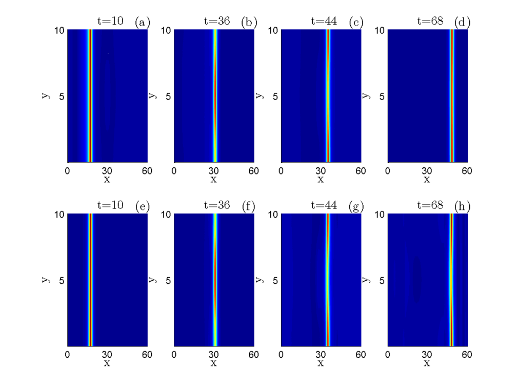
Figure 2: (Colour online) Contour plot of the time evolution of the Josephson phase derivative in the $L=60\times w=10$ junction with the rectangular impurity (4) with $\mu=0.5$, $d_{x}=3$, $d_{y}=5$, $\alpha=0.1$, $\gamma=0.08$ [(a)-(d)] and $\alpha=0.01$, $\gamma=0.008$ [(e)-(h)].

The fluxon retrapping current was computed numerically as well, showing its steady decay when the junction width was increased. These results will be discussed in detail in the next subsection.

The following conclusions can be drawn from these results. The fluxon shape experiences certain changes after passing the impurities, namely the redistribution of the Josephson phase along the fluxon line in the $y$ direction, as well as the slight bending of the fluxon shape in the same direction. These distortions eventually die out after some time, for $\alpha=0.05$ and $\alpha=0.1$ this happens quite soon after the passage through the impurity. For smaller dissipation ($\alpha=0.01$, as shown in Figs. 1i-l) the oscillations of the Josephson phase along the $y$ direction seem to survive for much longer time, comparable with the fluxon propagation time along the junction. The numerical simulations for thinner junctions, $w<10$ (not shown in the paper), demonstrate that these shape distortions are much weaker and are hardly noticeable. Thus, when studying the Q1D fluxon interaction with impurities one can assume with the high degree of certainty that the fluxon is an almost hard rod at least if $w\sim{\cal O}(1)$. Due to finiteness of the junction in the $y$ direction and the boundary conditions (5), the straight soliton front is the energetically most favourable solution and thus it is not possible to observe the arc-like solitons reported in [16].

3.2 Retrapping current calculation

Similarly to fluxon propagation in the 1D LJJ [4, 5, 6], there must exist two characteristic values of the bias current, $\gamma_{c}$ and $\gamma_{thr}$, $\gamma_{c}>\gamma_{thr}$. Moreover, the current-voltage characteristics of the LJJ with impurities have hysteretic nature [5, 6]. If $\gamma>\gamma_{c}$, the pinning on the impurity is not possible and there exists only one attractor that corresponds to fluxon propagation. This happens because the bias current is too strong for the fluxon to get trapped on the impurity. In the interval $\gamma_{thr}<\gamma<\gamma_{c}$, at least two attractors coexist: one corresponds to fluxon pinning on the impurity (there can be several different pinned fluxons if the impurity has finite length [9]) and another one to fluxon propagation. If $\gamma<\gamma_{thr}$, the only possible regime is fluxon pinning on the impurity. The value of $\gamma_{c}$ is defined only by the properties of the impurity, and can be obtained directly from the 1D analog. Contrary, for the retrapping current the dimensionality of the junction and its width are crucial.

Far from the impurity, the fluxon kinetic energy is proportional to the junction width and equals $E_{k}=8w[(1-v_{\infty}^{2})^{-1/2}-1]$. Here, $v_{\infty}=[1+(4\alpha/(\pi\gamma))^{2}]^{-1/2}$ is the equilibrium fluxon velocity in the spatially homogeneous LJJ [4]. In the non-relativistic fluxon case ($|v_{\infty}|\ll 1$), one gets $v_{\infty}\simeq\pi\gamma/(4\alpha)$. By substituting the ansatz
$\phi(x,y;t)=4\arctan\;\exp\{\left[x-X(y,t)\right]/\sqrt{1-v^{2}}\}$ into Eq. (1), where $X(y,t)$ is the coordinate of the fluxon center of mass, one can obtain the Newtonian equation of motion for the fluxon center.

Since the fluxons under consideration are extended objects in the $y$ direction, the equation for the center of mass dynamics as well as the impurity potential should depend on $y$. Taking into account the numerical simulation in the previous section, we consider the fuxon as an absolutely rigid rod. We also mention that the impurity function $f(x,y)$ can be factorised in the cases (3)-(5), therefore its center of mass dynamics can be effectively projected on the $x$ axis and the respective equation of motion can be written as

$$m{\ddot{X}}+m\alpha{\ddot{X}}+\frac{\partial U(X)}{\partial X}=0,~{}U(X)=-2\pi\gamma X+U_{0}(X)\;,$$ (6)

where the center of mass coordinate $X$ depends only on time. The impurity potential $U_{0}(X)$ now can be calculated from the respective 1D problem by simply taking away the $y$-dependent part in Eqs. (2)-(4). The fluxon mass $m$ has to be rescaled depending on the type of the impurity. In the pure 1D case $m=8$. This assumption works well only if the impurity is consists of lines and/or rectangles. If it has a more complex shape, for example, like triangle, the projection on the 1D problem becomes more complicated.

Point impurity. In the point impurity case (2), we consider the line of $N$ identical equidistant impurities with $a_{n}=0$, $n=1,2,\ldots,N$ which are placed symmetrically with respect to the central line $y=0$. Each impurity creates the potential $2\mu/\cosh^{2}{X}$. In order to project the problem on the 1D picture it is necessary to rescale the fluxon mass from $m=8$ to $m=8w/N$, thus within the kinematic approach the retrapping current can be found as a root of the energy balance equation $E_{k}=2\mu$, where $E_{k}=m[(1-v_{\infty}^{2})^{-1/2}-1]\simeq 4wv_{\infty}^{2}/N+{\cal O}(v_{\infty}^{4})$ is the fluxon kinetic energy. In the non-relativistic case one gets $\gamma_{thr}\simeq({\alpha}/{\pi})\sqrt{{8\mu N}/{w}}$. The correction of the order ${\cal O}(\alpha^{2})$ can be taken into account with the help of the method, developed in [5]. The modification of this method for the Q1D case is straightforward, therefore we describe only the main steps. The improved energy balance relation equates the fluxon energy at $X=-\infty$ and its losses due to the dissipation, $\Delta E$, with the maximal height of the potential barrier $U(X)$:

$$m\left({\pi\gamma\over{2\alpha}}\right)^{2}+\Delta E=U(X_{max}),$$ (7)

where $X_{min}$, $X_{max}>X_{min}$ are the extrema of the potential $U(X)$, $X_{min}\simeq-\ln(\mu/\gamma)/2$, $X_{max}\simeq-\pi\gamma/(2\mu)$. Equation (7) is universal and will be used for all types of impurities. The energy loss due to the dissipation equals
$\Delta E=8\alpha wN^{-1}\int_{-\infty}^{X_{max}}(v_{\infty}-\dot{X})dX\simeq 4\ln 2\sqrt{2\mu w}\alpha$. Inserting this correction term $\Delta E$ into the improved energy balance equation and keeping the terms up to the order ${\cal O}(\alpha^{2})$, one gets the final corrected expression for the retrapping current:

$$\gamma_{thr}\simeq\frac{\alpha}{\pi}\left(\sqrt{\frac{8\mu N}{w}}-4\alpha\ln 2\right).$$ (8)

It appears that the $\gamma_{thr}(w)$ relation is obtained simply by dividing the impurity strength by the factor $w/N$, moreover, the ${\cal O}(\alpha^{2})$ correction does not depend on the junction width at all. From this expression one can clearly see that if only the ${\cal O}(\alpha)$ term is taken into account, the retrapping current disappears as $w\to\infty$, thus, in the infinitely wide junction a fluxon always passes the impurity. The second term in Eq. (8) does not depend on $w$, and, therefore it may lead to the wrong conclusion that $\gamma_{thr}$ does not tend to zero as $w\to\infty$. However, it should be noted that this term has been derived under the assumption of $w$ being finite.

The numerical simulations confirm the main suggestion of this Letter: the retrapping current decays with the growth of the junction width. The approximate expression (8) appears to be in good agreement with the numerical data for smaller values of $w$, while for larger $w$’s the numerical and analytic data diverge (however, the agreement remains to be satisfactory). All this is presented in Fig. 1a where the analytic results are given by solid lines and the numerical data are shown by markers. In the case of two and three impurities, placed along the line in the $y$ direction, the retrapping current virtually does not depend on the distance $a_{y}$ between them. For instance, the markers that correspond to $a_{y}=2$ ($\times$), $a_{y}=3$ ($\circ$), $a_{y}=4$ ($\blacklozenge$) at $N=2$ and $w=5$ are almost indistinguishable.

One may consider the excentrically placed (i.e., lying away from the $x=0$ axis) impurity. The kinematic approach does not distinguish the impurities, placed at the different positions. The numerical simulations show that the difference between the retrapping currents in both the cases is very small. For example, $\gamma_{thr}=0.03770$ for the centrally placed impurity, $a_{1}=b_{1}=0$, at $w=2$ (the rest of the parameters are as in Fig. 1a) and $\gamma_{thr}=0.03776$ for the impurity at $a_{1}=0$, $b_{1}=w/4$ .

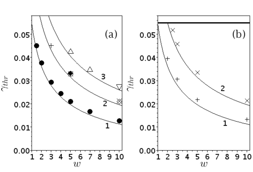
Figure 3: Retrapping current as a function of the junction width $w$ for $\alpha=0.1$, $\mu=0.5$. Panel (a) corresponds to the case of point impurities (2) with solid lines illustrating the approximate formula (8) at $N=1$ (line 1), $N=2$ (line 2) and $N=3$ (line 3). Markers correspond to the results of numerical simulations at $N=1$ ($\bullet$); $N=2$ with $a_{y}=1$ ($+$), $a_{y}=2$ ($\times$), $a_{y}=3$ ($\circ$), $a_{y}=4$ ($\blacklozenge$) and $a_{y}=7$ ($\diamond$); $N=3$ with $a_{y}=1$ ($\Delta$) and $a_{y}=2$ ($\nabla$). Panel (b) corresponds to the case of the line impurity (3) with $d_{y}=1$ (1 and $+$) and $d_{y}=2$ (2 and $\times$). Markers correspond to numerical results and solid lines correspond to the formula (9). Thick horizontal line corresponds to the retrapping current on the point microshort in the pure 1D case.

Line impurity. In the case of the impurity line (3), the same energy balance expression holds as for the point impurity but the fluxon mass is assumed to be $m=8w/d_{y}$. The rest of the calculation procedure for the retrapping current is the same as for the point impuritiy. As a result, we obtain the the final expression for the retrapping current:

$$\gamma_{thr}=\frac{\alpha}{\pi}\left(\sqrt{\frac{8\mu d_{y}}{w}}-4\alpha\ln 2\right)~{}.$$ (9)

Numerically computed $\gamma_{thr}$ appears to be in good correspondence with the approximate expression (9) as shown in Fig. 3b. Similarly to the point impurity case, the discrepancy between the analytical and numerical results increases at larger $w$. In the limit $d_{y}/w\to 1$, the effective 1D picture is restored because the impurity strip crosses the whole junction in the $y$ direction. Thus, the retrapping current attains the value $\gamma_{thr}={\alpha}(\sqrt{8\mu}-4\alpha\ln 2)/\pi$ for the 1D soliton case (shown by the thick horizontal line in Fig. 3b). Thus, we observe that if the strip impurity consitutes, for example, about $1/3$ of the junction width, the retrapping current is about $40\%$ less than the respective 1D value.

Rectangular impurity. Finally, we consider the rectangular impurity (4). In the point-particle description, the fluxon “feels” this impurity as the potential $U_{0}(X)=2\mu[\tanh(X+d_{x}/2)+\tanh(d_{x}/2-X)]$ [7]. In this case, the energy balance reads $8w[(1-v_{\infty}^{2})^{-1/2}-1]=4\mu d_{y}\tanh(d_{x}/2)$, from which the expression for the threshold current can be easily computed. For large $d_{x}$ it can be complemented by the correction ${\cal O}(\alpha^{2})$ computed for the 1D case in [7, 8]. The fluxon mass should be renormalized as $8\to 8w/d_{y}$. In this limit it is assumed that the impurity creates the step-like potential $U_{0}(X)=2\mu[\tanh X+1]$, which has a minimum at $X_{min}=-\mbox{arcsech}\sqrt{\pi\gamma/\mu}$ and a maximum at $X_{max}=\mbox{arcsech}\sqrt{\pi\gamma/\mu}$. The energy losses due to the dissipation $\Delta E=8\alpha wd_{y}^{-1}\int_{-\infty}^{X_{max}}(v_{\infty}-{\dot{X}})dX\simeq 4\sqrt{\mu d_{y}w^{-1}}\alpha\{\ln[\mu/(\pi\gamma)]+{\cal O}(1)\}$ should be substituted in the energy balance equation (7). The final approximation reads

$$\gamma_{thr}=\frac{\alpha}{\pi}\sqrt{\frac{d_{y}}{w}}\left[4\sqrt{\mu\tanh(d_{x}/2)}-\alpha\ln\left({\mu\over\alpha^{2}}\frac{w}{d_{y}}\right)\right].$$ (10)

Note that at variance with the point and line impurities, the second correction depends on the both junction and the impurity width. In the 1D limit ($d_{y}/w\to 1$), the formula (10) retains the form, found in [7, 8]. In the limit $w\to\infty$, the second term decays to zero, but much slower than the decay law ${\cal O}(w^{-1/2})$ of the first term. Once again, the second term is a correct approximation only for finite values of $w$.

In the opposite limit, $d_{x}\to 0$, one can use the following approximation: $\tanh(X+d_{x}/2)+\tanh(d_{x}-X)=\sinh d_{x}/[\cosh^{2}X+\sinh^{2}(d_{x}/2)]\simeq d_{x}\mbox{sech}^{2}X+{\cal O}(d_{x}^{2})$. Thus, the effective potential $U(X)$ is approximately the same as for the line impurity up to the coefficient $\sinh{d_{x}}\simeq d_{x}$. Therefore the formula (9) can be modified accordingly and finally the retrapping current reads

$$\gamma_{thr}=\frac{\alpha}{\pi}\left[4\sqrt{\frac{\mu d_{y}d_{x}/2}{w}}-4\alpha\ln 2\right].$$ (11)

The results of numerical simulations given in Fig. 4 demonstrate satisfactory correspondence with the analytical approximations (10)-(11).

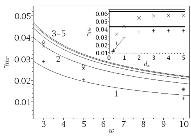
Figure 4: Retrapping current as a function of the junction width $w$ for the rectangular impurity (4) at $\alpha=0.1$, $\mu=0.5$ and $d_{y}=1$. The markers correspond to the cases $d_{x}=1$ ($+$), $d_{x}=2$ ($\times$), $d_{x}=3$ ($\oplus$), $d_{x}=4$ ($\diamond$) and $d_{x}=5$ ($\blacklozenge$). The analytical approximation (10) is given by the solid lines $1-5$ for $d_{x}=1,2,\ldots,5$, respectively. The inset shows the retrapping current dependence on $d_{x}$ at $d_{y}=1$ ($+$), $d_{y}=2$ ($\times$) and $w=3$. Two thick solid lines correspond to the analytical approximation (10) at $d_{x}\to\infty$ for $d_{y}=1$ and $d_{y}=2$, thin solid line corresponds to the approximation (11) at $d_{y}=1$.

The deviations from the numerical results appear to be stronger as compared to the point and line impurities, mostly because we were unable to provide the ${\cal O}(\alpha^{2})$ correction that works equally well in both limits $d_{x}\to 0$ and $d_{x}\to\infty$ and also due to higher degree of the fluxon deformation during the interation with the impurity. It should be mentioned that even for $d_{x}\gtrsim 3$ one can consider the “long” $d_{x}$ limit and it works fairly well. Indeeed, the markers that correspond to $d_{x}=3$ ($\oplus$), $d_{x}=4$ ($\diamond$) and $d_{x}=5$ ($\blacklozenge$) seem to be almost indistinguishable in Fig. 4.

4 Discussion and conclusion

To summarize, we have shown that quasi-one-dimensional fluxon passage across microshorts is significantly enhanced in comparison with the purely one-dimensional case. The retrapping threshold current decays with the junction width approximately as $w^{-1/2}$, according to the kinematic approach. The numerical simulations support this dependence for intermediate (several $\lambda_{J}$) values of $w$. With the increase of $w$, the discrepancy between the numerical results and the kinematic approximation becomes more distinct. The reason of this discrepancy lies in the fact that for $w\gg 1$ the fluxon cannot be longer considered as an completely rigid object and its deformation the $y$ direction should be taken into account.

One can formulate the following simple argument that explains the enhanced fluxon transmission across the obstacle of the width $d_{y}$ in the Q1D case. The obstacle can be described as a localized (both in the $x$ and $y$ directions) potential barrier. Only the central part ($|y|\gtrsim d_{y}/2$) of the initially homogeneous in the $y$ direction fluxon takes part in the interaction process, while the marginal areas $d_{y}/2\lesssim|y|\leq w/2$ do not. Thus, if the energy in the tails is sufficient enough to overcome the barrier, the fluxon will pass. If $w\to\infty$, the energy in the non-interacting part of the fluxon tends to infinity, and, consequently, it will overcome any localized obstacle.

Finally, we would like to outline the future research directions. In our opinion they lie beyond the rigid rod approximation used in this Letter. In this case the fluxon center of mass depends also on the transverse coordinate $y$ and the effective equations of motion are PDE’s and not ODE’s, like Eq. (6). Accounting for the dependence on $y$ becomes important in the following cases: (i) the junction width is too large and the flexural oscillations along the fluxon line appear; (ii) the dissipation is rather small and/or the junction length is $L\sim w$, thus the spatial distortions of the fluxon line do not have enough time to die out. These cases are also interesting in connection with the arc-like fluxons found in the infinitely wide junction [16] and the variety of the excitations that travel along the fluxon crest in the dissipationless 2D junctions [17]. The combined effect of the dissipation and the finite junction width makes the transverse-invariant fluxon front the energetically most favourable solution. However, other attractors of the system which are non-transverse-invariant may exist as suggested by Figs. 1j-l, especially when dissipation is small. Finding them and investigating how they will manifest themselves on the junction current-voltage dependence is an important problem.

References

- [1] A. Barone and G. Paterno, Physics and Applications of the Josephson Effect, Wiley, New York, 1982.
- [2] K. K. Likharev, Dynamics of Josephson Junctions and Circuits, Gordon and Breach, New York, 1986.
- [3] A. V. Ustinov, Physica D 123 (1998) 315.
- [4] D. W. McLaughlin, A. C. Scott, Phys. Rev. A 18 (1978) 1652.
- [5] Yu. S. Kivshar, B. A. Malomed, A. A Nepomnyashchy, Eksp. Teor. Fiz. 94 (1988) 356 [Sov. Phys. JETP 67 (1988) 850].
- [6] B. A. Malomed, A. V. Ustinov, J. Appl. Phys. 67 (1990) 3791.
- [7] Yu. S. Kivshar, A. M. Kosevich, O. A. Chubykalo, Phys. Let. A 129 (1988) 449.
- [8] Yu. S. Kivshar, B. A. Malomed, J. Appl. Phys. 65 (1989) 879.
- [9] G. Derks, A. Doelman, C. J. K. Knight, H. Susanto, Eur. J. Appl. Math 23 (2012) 201.
- [10] S. Sakai, H. Akoh and H. Hayakawa, Japan. J. Appl. Phys. 24 (1985) L771; H. Akoh, S. Sakai, A. Yagi and H. Hayakawa, IEEE Trans. Magn. 21 (1985) 737; I.L. Serpuchenko and A.V. Ustinov, Pis’ma Zh. Eksp. Teor. Fiz. 46 (1987) 435 [Sov. Phys. JETP Lett. 46 (1987) 549].
- [11] E. Goldobin et al, Phys. Rev. B 72 (2005) 054527.
- [12] A. Fedorov, A. Shnirman, G. Schön, G. S. A. Kidiyarova-Shevchenko, Phys. Rev. B 75 (2007) 224504.
- [13] P. L. Christiansen, O. H. Olsen, Phys. Let. A 68 (1978) 185; P. L. Christiansen, P. S. Lomdahl, Physica D 2 (1981) 482.
- [14] A. Benabdallah, J. G. Caputo, N. Flytzanis, Physica D 161 (2002) 79.
- [15] J. G. Caputo, Y. Gaididei, Physica C 402 (2004) 160.
- [16] B. A. Malomed, Physica D 52 (1991) 157.
- [17] D. R. Gulevich et al, Phys. Rev. Lett. 101 (2008) 127002; Phys. Rev. B 80 (2008) 094509.
- [18] B. Piette, W. J. Zakrzewski, J. Brand, J. Phys. A: Math. Gen. 38 (2005) 10403.
- [19] Y. Zolotaryuk, A. V. Savin, P. L. Christiansen, Phys. Rev. B 57 (1998) 14213.
- [20] Y. S. Kivshar, Z. Fei, L. Vazquez, Phys. Rev. Lett. 67 (1991) 1177; Y. S. Kivshar et al, J. Phys. A: Math. Gen. 25 (1992).
- [21] J. H. Al-Alawi, W. J. Zakrzewski, J. Phys. A: Math. Theor. 40 (2007) 11319.