On the Generalized Delay-Capacity Tradeoff of Mobile Networks with Lévy Flight Mobility

Abstract

In the literature, scaling laws for wireless mobile networks have been characterized under various models of node mobility and several assumptions on how communication occurs between nodes. To improve the realism in the analysis of scaling laws, we propose a new analytical framework. The framework is the first to consider a Lévy flight mobility pattern, which is known to closely mimic human mobility patterns. Also, this is the first work that allows nodes to communicate while being mobile. Under this framework, delays ($\bar{D}$) to obtain various levels of per-node throughput $(\lambda)$ for Lévy flight are suggested as $\bar{D}(\lambda)=O(\sqrt{\min(n^{1+\alpha}\lambda,n^{2})})$, where Lévy flight is a random walk of a power-law flight distribution with an exponent $\alpha\in(0,2]$. The same framework presents a new tighter tradeoff $\bar{D}(\lambda)=O(\sqrt{\max(1,n\lambda^{3})})$ for i.i.d. mobility, whose delays are lower than existing results for the same levels of per-node throughput.

I Introduction

Since the work in [1] that showed that mobility can be exploited to improve network throughput, there has been a plethora of work on this subject. A major effort in this direction has been in the design of delay tolerant networks (DTNs). However, this benefit in throughput comes at a significant delay cost. The amount of delays required to achieve a level of throughput for various mobility models such as i.i.d. mobility, random waypoint (RWP), random direction (RD), and Brownian motion (BM) have been extensively studied in [2, 3, 4, 5, 6]. Specifically, the delay required for constant per-node throughput has been shown to grow as $\Theta(n)$, which scales as fast as the network size $n$, for most mobility models including i.i.d. mobility, RWP, RD, and BM [7, 2, 5, 8]. Despite significant advances in the development of delay-capacity scaling laws, there has been considerable skepticism regarding the applicability of the results to real mobile networks because of various simplifying assumptions used in the analysis.

In this paper, we address two issues towards making the delay-capacity tradeoff analysis more realistic: 1) contacts among nodes in the middle of their movements and 2) Lévy mobility patterns of nodes in the network. In the literature, for mathematical simplicity, existing results have assumed that nodes show slotted movements, and they do not communicate with each other while being mobile. Thus, they make contacts with other nodes and transfer data only at the edge of time slots. In other words, as shown in Fig. 1 (a), the opportunity for meeting other nodes during mobility has been ignored, although such opportunities can substantially reduce packet delivery delays. Also, in this work we focus on the Lévy flight model, which is widely accepted to closely mimic the actual movement of humans [9, 10]. The trajectory of this model is illustrated in Fig. 1 (b). To enhance the realism in the analysis of delay-capacity tradeoff, we develop a new analytical framework which takes both of these factors into account by developing a technique that characterizes the distribution of “first meeting time” among nodes conforming to Lèvy flight mobility in a two-dimensional space. It is important to note that the exact distribution of the first meeting time of Lévy flight even in a one-dimensional space has been an open problem even though it has applicability in a diverse set of research problems (e.g., characterization of particle movements and animal movements) in physics and mathematics. It is also informative to note that the distribution of the first meeting time of BM, which can be considered as an extreme case of Lévy flight, is also an open problem as noted in [11, 12].

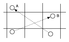
(a) Contacts while being mobile

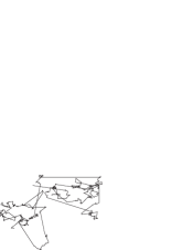
(b) A trajectory of Lévy flight

Figure 1: Our considerations for improving the realism of delay-capacity tradeoff: (a) Conventionally, nodes $A$ and $B$ are assumed to have no contact opportunity, but we consider they can meet each other even during their movements. (b) We also consider that nodes follow Lévy flight mobility.

Lévy flight, the mobility model we focus on in this paper, is a subset of Lévy mobility in which a node moves from position to position in a constant time. Another special case, Lévy walk, in which a node moves from one position to another in time proportional to the distance between the positions. Except for the notion of the time required for each movement, Lévy flight and Lévy walk are fundamentally the same random walk whose flight length distribution asymptotically follows a power-law $f_{\alpha}(z)\approx 1/z^{\alpha+1}$, where $z$ and $\alpha$ denote the flight length (i.e., moving distance of each slotted movement) and the power-law slope ranging $0<\alpha<2$, respectively. The heavy-tailed movements of Lévy mobility render the delay characterization extremely challenging. Our framework addresses these challenges using theories from stochastic geometry and probability, and provides a delay-capacity tradeoff for Lévy flight. Also, for a simpler i.i.d. mobility model, we provide a tighter delay-capacity tradeoff compared to existing studies using the same framework.

Fig. 2 and Table I summarize the new tradeoffs identified using our analytical framework. The results show that the tradeoff for Lévy flight follows $\bar{D}(\lambda)=O(\sqrt{\min\{n^{1+\alpha}\lambda,n^{2}\}})$ to obtain a per-node throughput of $\lambda=\Theta(n^{-\eta})\,(0\leq\eta\leq 1/2)$ as shown in Figs. 3 (a) and (b). These results are well aligned with the critical delay (i.e., minimum delay required to achieve $\lambda=\omega(1/\sqrt{n})$) suggested in [13]. Our tradeoffs show an important finding that the delay required to obtain constant per-node throughput (i.e., $\lambda=\Theta(1)$) can be smaller than $\Theta(n)$ in mobile networks with mobility models such as Lévy flight with $\alpha<1$ and i.i.d. mobility. This is an important observation given that most of the existing studies present the delay required to obtain constant per-node throughput to be $\Theta(n)$ for almost all mobility models including the i.i.d. mobility.

Our tradeoff for Lévy flight becomes especially more interesting when we input $\alpha$ values from measurements presented in Table II into the tradeoff. This gives us a hint on how the performance of the network will scale in reality when the network consists of devices mainly carried (or driven) by humans. For $\alpha$ values between 0.53 and 1.81, the delays to obtain $\lambda=\Theta(1)$ are expected to lie between $O(n^{0.77})$ and $O(n)$. This implies that in reality, a DTN mainly operated by human mobility may indeed experience less than $\Theta(n)$ delay in some areas. This observation of smaller delay suggests that mobile networks relying on opportunistic transmissions may have higher practical values in reality given that the delays have been overestimated by mobility and contact models with less realism.

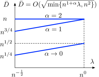
(a) Lévy flight

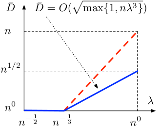
(b) i.i.d. mobility

Figure 2: (a) The delay-capacity tradeoffs for Lévy flight with various $\alpha$ obtained from our analytical framework and (b) the new tradeoff for i.i.d. mobility (solid line) shown together with the previously known tradeoff (dotted line).

TABLE I: The new delay-capacity tradeoffs identified using our analytical framework for Lévy flight and i.i.d. mobility

Mobility	Tradeoff $\bar{D}(\lambda)$	$\bar{D}(\lambda)$ for $\lambda=\Theta(1)$
Lévy flight	$O(\sqrt{\min(n^{1+\alpha}\lambda,n^{2})})$	$O(\sqrt{\min(n^{1+\alpha},n^{2})})$
i.i.d.	$O(\sqrt{\max(1,n\lambda^{3})})$	$O(n^{1/2})$

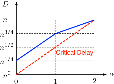
(a) $\lambda=\Theta(1/\sqrt{n})$

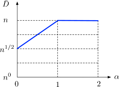
(b) $\lambda=\Theta(1)$

Figure 3: The upper bounds on $\bar{D}(\lambda)$ for Lévy flight with $\alpha\in(0,2]$ to obtain (a) $\lambda=\Theta(1/\sqrt{n})$ and (b) $\lambda=\Theta(1)$. The critical delay for Lévy flight derived in [13] is depicted in (a).

TABLE II: Experimental $\alpha$ values from five sites presented in [9]. These values are from experimental GPS traces from five sites with more than 100 participants in total.

Site	$\alpha$	Site	$\alpha$	Site	$\alpha$
KAIST	0.53	New York	1.62	State fair	1.81
NCSU	1.27	Disney World	1.20

The rest of the paper is organized as follows. We overview a list of related work in Section II and introduce our system models and definitions of performance metrics in Section III. We then provide the intuition on how our analytical framework evaluates delay-capacity tradeoff using the properties of first meeting time of random walks in Section IV. Based on the understanding in Section IV, we analyze the tradeoffs of Lévy flight and i.i.d. mobility models in Sections V and VI, respectively. After briefly concluding our work in Section VII, we provide full details of proofs used in Sections V and VI through Appendices.

II Related Work

In [14], it was shown that the per-node throughput of random wireless networks with $n$ static nodes scales as $O(1/\sqrt{n})$. The result was later enhanced to $\Theta(1/\sqrt{n})$ by exercising individual power control [15]. Grossglauser and Tse [1] proved that constant per-node throughput is achievable by using mobility when nodes follow ergodic and stationary mobility models. This contradicted the conventional belief that node mobility negatively impacts network capacity due to interruptions in connectivity.

Many follow-up studies [16, 17, 18, 2, 7, 4, 5] have been devoted to characterize and exploit the delay-capacity tradeoffs. In particular, the delay required to obtain constant per-node throughput has been studied under various mobility models [2, 3, 4, 5, 6]. The key message is that the delay of 2-hop relaying proposed in [1] is $\Theta(n)$ for most mobility models such as i.i.d. mobility, RD, RWP, and BM.

The delay-capacity tradeoff for per-node throughput $\lambda=\Theta(n^{-\eta})\,(0\leq\eta\leq 1/2)$ is first presented in [19] as $\bar{D}(\lambda)=O(n\lambda)$ for RWP model. In [5], the authors identified that $\bar{D}(\lambda)=\Theta(\max(1,n\lambda^{3}))$ holds for i.i.d. mobility. Later, [8] showed that $\bar{D}(\lambda)=\Theta(n)$ holds for BM irrespective of $\lambda$.

More realistic mobility models, Lévy mobility models known to closely capture human movement patterns, were first analyzed in [13] for a special case of the tradeoff. Using spatio-temporal probability density functions, the critical delay defined by the minimum delay required to achieve larger throughput than $\Theta(1/\sqrt{n})$ is identified for Lévy flight as well as Lévy walk.

Existing results on delay-capacity tradeoffs for mobile networks have been built under the assumption that nodes are able to communicate with each other only at the edge of time slots for slotted movements. Also, there has been no framework which can fully understand the delay-capacity tradeoff for Lévy mobility. In this paper, we develop an analytical framework which handles both of these issues and are able to use this framework to characterize the delay-capacity tradeoff.

III System Model

III-A Network Model

We consider a wireless mobile network indexed by $n\in\mathbb{N}\triangleq\{1,2,\ldots\}$, where, in the $n$th network, $n$ nodes move on a completely wrapped-around disc $\bm{\mathcal{D}}\,(\subset\mathbb{R}^{2})$ whose radius scales as $\Theta(\sqrt{n})$. Without loss of generality, we set the radius and the center of the disc $\bm{\mathcal{D}}$ as $\sqrt{n}$ and $\bm{0}\triangleq(0,0)$, respectively, i.e., $\bm{\mathcal{D}}=\{\bm{x}\in\mathbb{R}^{2}\,|\,|\bm{x}|\leq\sqrt{n}\}$. We assume that the density of the network is fixed to 1 as $n$ increases. We also assume that all nodes are homogeneous in that each node generates data with the same intensity to its own destination. The packet generation process at each node is independent of node mobility. The generated packets are assumed to have no expiration until their delivery and the size of each node’s buffer is assumed to be unlimited. Each packet can be delivered by either direct one-hop transmission or over multiple hops using relay nodes.

To model interference in wireless networks, we adopt the following protocol model as in [6, 14]. Let $\bm{X}_{i}(t)$ denote the location of node $i\,(=1,\ldots,n)$ at time $t\,(\geq 0)$. Let $L_{(i,j)}(t)\triangleq|\bm{X}_{i}(t)-\bm{X}_{j}(t)|$ denote the Euclidean distance between nodes $i$ and $j$ at time $t$. Under the protocol model, nodes transmit packets successfully at a constant rate $W$ bits/sec, if and only if the following is satisfied: for a transmitter $i$, a receiver $j$ and every other node $u\neq i,j$ transmitting simultaneously,

$$L_{(u,j)}(t) \geq(1+\Delta)\,L_{(i,j)}(t),$$

where $\Delta$ is some positive constant. In addition, the distance between nodes $i$ and $j$ at time $t$ should satisfy $L_{(i,j)}(t)\leq r$, where $r\,(>0)$ denotes the maximum communication range. We assume the fluid packet model [6], which allows concurrent transmissions of node pairs (with the rate divided by the number of pairs) interfering each other. We denote by $\Pi$ the class of all feasible scheduling schemes conforming our descriptions.

III-B Mobility Model

In this subsection, we mathematically describe the Lévy flight model and the i.i.d. mobility model. At time $t=0$, node $i$ chooses its location uniformly on the disc $\bm{\mathcal{D}}$ (i.e., $\bm{X}_{i}(0)\sim\text{Uniform}(\bm{\mathcal{D}})$), which is independent of the others $\bm{X}_{j}(0)$ for $j\neq i$. We assume that time is divided into slots of unit length and is indexed by $k\in\mathbb{N}$. At the beginning of the $k$th slot (i.e., at time $t=k-1$), node $i$ chooses its next slotted location $\bm{X}_{i}(k)$ according to the associated mobility model. During the $k$th slot (i.e., during time $t\in(k-1,k]$), node $i$ moves from $\bm{X}_{i}(k-1)$ to $\bm{X}_{i}(k)$ with a constant velocity. Thus, $\bm{X}_{i}(k-1+\delta)$ for $\delta\in(0,1)$ is determined by $\bm{X}_{i}(k-1)$ and $\bm{X}_{i}(k)$ as follows:

$$\bm{X}_{i}(k-1+\delta) =(1-\delta)\bm{X}_{i}(k-1)+\delta\bm{X}_{i}(k).$$ (1)

Lévy Flight Model. At the beginning of the $k$th slot (i.e., at time $t=k-1$), node $i$ chooses flight angle and flight length, denoted by $\theta_{i}(k)\,(\in(0,2\pi])$ and $Z_{i}(k)\,(>0)$, respectively. During the $k$th slot (i.e., during time $t\in(k-1,k]$), node $i$ moves from $\bm{X}_{i}(k-1)$ to the selected direction $\theta_{i}(k)$ of the distance $Z_{i}(k)$. Thus, the location $\bm{X}_{i}(k)$ is determined as

$$\bm{X}_{i}(k) =\bm{X}_{i}(k-1)+\bm{V}_{i}(k),$$ (2)

where

$$\bm{V}_{i}(k)\triangleq\big{(}Z_{i}(k)\cos\theta_{i}(k),Z_{i}(k)\sin\theta_{i}(k)\big{)}.$$ (3)

The flight angle $\theta_{i}(k)$ and the flight length $Z_{i}(k)$ are independent of each other and also independent of the previous locations $\bm{X}_{i}(t)$ for the times $t\in[0,k-1]$ before they are generated. Hence, $\bm{V}_{i}(k)$ is independent of $\bm{X}_{i}(t)$ for all $t\in[0,k-1]$.

Each flight angle $\theta_{i}(k)$ and flight length $Z_{i}(k)$ are independent and identically distributed across node index $i$ and slot index $k$. Let $\theta$ and $Z$ be a generic random variable for $\theta_{i}(k)$ and $Z_{i}(k)$, respectively. Then, the flight angle $\theta$ is uniformly distributed over $(0,2\pi]$, and the flight length $Z$ is generated from a random variable $Z^{\star}$ having the Lévy $\alpha$-stable distribution [20] by the relation $Z=|Z^{\star}|$. The probability density function of $Z^{\star}$ is given by

$$f_{Z^{\star}}(z)=\frac{1}{2\pi}\int_{-\infty}^{\infty}e^{-izt}\varphi_{Z^{\star}}(t)\,\text{d}t,$$ (4)

where $\varphi_{Z^{\star}}(t)\triangleq\text{E}[e^{itZ^{\star}}]$ is the characteristic function of $Z^{\star}$ and is given by $\varphi_{Z^{\star}}(t)=e^{-|st|^{\alpha}}$. Here, $|s|>0$ is a scale factor determining the width of the distribution, and $\alpha\in(0,2]$ is a distribution parameter that specifies the shape (i.e., heavytail-ness) of the distribution. The flight length $Z$ for $\alpha\in(0,1)$ has infinite mean and variance, while $Z$ for $\alpha\in[1,2)$ has finite mean but infinite variance. For $\alpha=2$, the Lévy $\alpha$-stable distribution reduces to a Gaussian distribution with a mean of zero and variance of $2s^{2}$, for which the flight length $Z$ has finite mean and variance.

Due to the complex form of the distribution, the Lévy $\alpha$-stable distribution for $\alpha\in(0,2)$ is often treated as a power-law type of asymptotic form:

$$f_{Z^{\star}}(z)\sim\frac{1}{|z|^{1+\alpha}},$$ (5)

where we use the notation $a(z)\sim b(z)$ for any two real functions $a(z)$ and $b(z)$ to denote $\lim_{z\to\infty}[a(z)/b(z)]=1$ [20]. The form (5) is known to closely approximate the tail part of the distribution in (4), and a number of papers in mathematics and physics, e.g., [21, 22], analyze Lévy mobility using the form (5). For mathematical tractability, in our analysis we will also use the asymptotic form (5). Specifically, we assume that there exist constants $c\,(>0)$ and $z_{\text{th}}\,(>0)$ such that

$$\text{P}\{Z>z\} =\frac{c}{z^{\alpha}},\quad\text{ for all }z\geq z_{\text{th}}.$$ (6)

i.i.d. Mobility Model. At the beginning of the $k$th slot (i.e., at time $t=k-1$), node $i$ chooses $\bm{X}_{i}(k)$ uniformly on the disc $\bm{\mathcal{D}}$, which is independent of its previous locations $\bm{X}_{i}(t)$ for the times $t\in[0,k-1]$ as well as the others $\bm{X}_{j}(k)$ for $j\neq i$. Thus, $\bm{X}_{i}(k)$ is independent and identically distributed across node index $i$ and slot index $k$.

III-C Contact Model

In our contact model, nodes are allowed to meet while being mobile. Hence, for a time $t^{\star}$ in a domain $\{t\,|\,t\geq 0\}$, we say that nodes $i$ and $j$ meet at time $t^{\star}$ (or are in contact at time $t^{\star}$) if they satisfy

$$L_{(i,j)}(t^{\star})\leq r.$$

In the widely adopted contact model where nodes are allowed to meet only at the end of their movements (i.e., at slot boundaries), a meeting event can occur for a time $k^{\star}$ in a domain $\{k\,|\,k\in\{0\}\cup\mathbb{N}\}$ satisfying $L_{(i,j)}(k^{\star})\leq r$. We call this class of contact model slotted contact model throughout the paper.

Mobile nodes are exposed to more contact opportunities in our contact model compared to the slotted contact model.

III-D Performance Metrics

The key performance metrics of our interest are per-node throughput and average delay as defined next:

Definition 1 (Per-node throughput).

Let $\Lambda_{\pi:i}(t)$ be the total number of bits received at the destination node $i$ up to time $t$ under a scheduling scheme $\pi\in\Pi$. Let $\lambda_{\pi}$ be the per-node throughput under $\pi$. Then,

$$\lambda_{\pi} \triangleq\liminf_{t\rightarrow\infty}\frac{1}{n}\sum_{i=1}^{n}\frac{\Lambda_{\pi:i}(t)}{t}.$$

Definition 2 (Average delay).

Let $D_{\pi:i,v}$ be the time taken for the $v$th packet generated from the source node $i$ to arrive at its destination node under a scheduling scheme $\pi\in\Pi$. Let $\bar{D}_{\pi}$ be the average delay under $\pi$. Then,

$$\bar{D}_{\pi} \triangleq\lim_{w\rightarrow\infty}\frac{1}{n}\sum_{i=1}^{n}\frac{1}{w}\sum_{v=1}^{w}D_{\pi:i,v}.$$

In this paper, we focus on analyzing the scaling property of the smallest average delay achieving per-node throughput $\lambda$. We call this minimum average delay optimal delay throughout this paper. We focus on the throughput only in the range from $\Theta(1/\sqrt{n})$ to $\Theta(1)$, since this range corresponds to the case where mobility can be used to improve the per-node throughput.

Definition 3 (Optimal delay).

Let $\bar{D}(\lambda)$ be the optimal delay to achieve per-node throughput $\lambda$. It is then given by

$$\bar{D}(\lambda) \triangleq\inf_{\{\pi\in\Pi\,|\,\lambda_{\pi}=\lambda\}}\bar{D}_{\pi}.$$

III-E Throughput Achieving Scheme

We now consider a scheme $\hat{\pi}$ that can realize per-node throughput $\lambda_{\hat{\pi}}$ scaling from $\Theta(1/\sqrt{n})$ to $\Theta(1)$. The scheme $\hat{\pi}$ operates as follows:

• When a packet is generated from a source node and the destination of the packet is within the communication range of the source node, the packet is transmitted to the destination node immediately.

• Otherwise, the source node broadcasts the packet to all neighboring nodes within its communication range. Note that this broadcast is only performed by the source node when the packet is generated.

• Any nodes carrying the packet can deliver the packet to the destination node when they are within the communication range of the destination node.

• When one of the packets (including the original packet and the duplicated ones) reaches the destination node, all others are not considered for delivery.

By appropriately scaling $r$ as a function of $n$, the scheme $\hat{\pi}$ can achieve per-node throughput $\lambda_{\hat{\pi}}$ ranging from $\Theta(1/\sqrt{n})$ to $\Theta(1)$, as shown in the following lemma.

Lemma 1.

Let the communication range $r$ scale as $\Theta(n^{\beta})$ $(0\leq\beta\leq 1/4)$. Then, the per-node throughput $\lambda_{\hat{\pi}}$ under the scheme $\hat{\pi}$ scales as $\Theta(n^{-2\beta})$.

Proof: If the network has been running for a long enough time, all nodes become to work as relay nodes and begin to have packets for all other nodes. Therefore, for a network with $n/a_{n}$ disjoint area where $a_{n}=\Theta(r^{2})$, all areas with more than two nodes can always be activated. Let $b_{n}$ denote the probability of having more than two nodes in an area. We then have

$$b_{n} =1-\left(1-\frac{a_{n}}{n}\right)^{n}-n\frac{a_{n}}{n}\left(1-\frac{a_{n}}{n}\right)^{n-1}.$$

In addition, the total network throughput becomes $b_{n}n/a_{n}$ and accordingly the per-node throughput is $\lambda_{\hat{\pi}}=b_{n}/a_{n}$. Without loss of generality, we assume $r=n^{\beta}\,(0\leq\beta\leq 1/4)$. Then, the per-node throughput $\lambda_{\hat{\pi}}$ is given by

$$\lambda_{\hat{\pi}} =n^{-2\beta}-n^{-2\beta}\left(1-n^{2\beta-1}\right)^{n}-\left(1-n^{2\beta-1}\right)^{n-1}.$$

In the following, we will show that

$$\lim_{n\to\infty}\frac{\lambda_{\hat{\pi}}}{n^{-2\beta}}$$

$$\quad=\lim_{n\to\infty}\big{\{}1\!-\!\left(1\!-\!n^{2\beta\!-\!1}\right)^{n}\!-\!n^{2\beta}\left(1\!-\!n^{2\beta\!-\!1}\right)^{n\!-\!1}\big{\}}$$ (7a)

$$\quad=\begin{cases}1-2\exp(-1),&\text{ if }\beta=0,\\ 1,&\text{ if }\beta\in(0,1/4].\end{cases}$$ (7b)

Hence, the per-node throughput $\lambda_{\hat{\pi}}$ under the scheme $\hat{\pi}$ scales as $\Theta(n^{-2\beta})$. Note that

$$\lim_{n\to\infty}\log(1-n^{2\beta-1})^{n} =\lim_{n\to\infty}n^{2\beta}\log(1-n^{2\beta-1})^{n^{1-2\beta}}$$

$$=\lim_{n\to\infty}n^{2\beta}\log(\exp(-1))$$

$$=\begin{cases}-1,&\text{ if }\beta=0,\\ -\infty,&\text{ if }\beta\in(0,1/4],\end{cases}$$

which gives

$$\lim_{n\to\infty}(1-n^{2\beta-1})^{n} =\begin{cases}\exp(-1),&\text{ if }\beta=0,\\ 0,&\text{ if }\beta\in(0,1/4].\end{cases}$$ (8)

Similarly,

$$\lim_{n\to\infty}\log\big{(}n^{2\beta}(1-n^{2\beta-1})^{n-1}\big{)}$$

$$=\lim_{n\to\infty}\big{\{}2\beta\log n+(n-1)n^{2\beta-1}\log(1-n^{2\beta-1})^{n^{1-2\beta}}\big{\}}$$

$$=\lim_{n\to\infty}\big{\{}2\beta\log n+n^{2\beta}\log(\exp(-1))\big{\}}$$

$$=\begin{cases}-1,&\text{ if }\beta=0,\\ -\infty,&\text{ if }\beta\in(0,1/4],\end{cases}$$

which gives

$$\lim_{n\to\infty}\!\!n^{2\beta}(1\!-\!n^{2\beta\!-\!1})^{n\!-\!1} =\begin{cases}\exp(-1),&\text{ if }\beta=0,\\ 0,&\text{ if }\beta\in(0,1/4].\end{cases}$$ (9)

By applying (8) and (9) to (7a), we have (7b). This complete the proof. $\blacksquare$

Let $\bar{D}_{\hat{\pi}}(\beta)$ be the average delay under $\hat{\pi}$ when $r=\Theta(n^{\beta})$. Lemma 1 implies that by setting $\beta=-\log_{n}(\sqrt{\lambda})$, the scheme $\hat{\pi}$ achieves the per-node throughput $\lambda_{\hat{\pi}}=\lambda$. Since the scheme $\hat{\pi}$ is of the class $\Pi$, the order of $\bar{D}(\lambda)$ can be obtained from $\bar{D}_{\hat{\pi}}(\beta)$ with the use of $\beta=-\log_{n}(\sqrt{\lambda})$, i.e.,

$$\bar{D}(\lambda) =\inf_{\{\pi\in\Pi\,|\,\lambda_{\pi}=\lambda\}}\bar{D}_{\pi}\leq\bar{D}_{\hat{\pi}}(-\log_{n}(\sqrt{\lambda})).$$ (10)

IV Preliminaries

In this section, we provide the key intuition to understand how our analytical framework utilizes the properties of first meeting time in the derivation of delay-capacity tradeoffs under the Lévy flight and the i.i.d. mobility models. We then sketch the challenges residing in our framework and briefly describe our approach to address these challenges.

IV-A Delay Analysis with First Meeting Time

The first meeting time of two nodes moving in a two-dimensional space, which is directly connected to $\bar{D}_{\hat{\pi}}$, is defined below:

Definition 4 (First meeting time).

For $i\neq j$, the first meeting time of nodes $i$ and $j$, denoted by $T_{(i,j)}$, is defined as

$$T_{(i,j)} \triangleq\inf\big{\{}t\geq 0\,\big{|}\,L_{(i,j)}(t)\leq r\big{\}}.$$

Since $T_{(i,j)}$ is independent and identically distributed across pair index $(i,j)$, we use $T$ to denote a generic random variable for $T_{(i,j)}$.

Let $D_{(s,d)}$ be a random variable representing the time taken by a packet generated from a source node $s$ to arrive at a destination node $d$. Since the packet generation process is independent of node mobility, we consider that each packet is generated at time $t=0$ without loss of generality. Then, the packet delay under the scheme $\hat{\pi}$, denoted by $D_{\hat{\pi}:(s,d)}$, can be expressed in terms of the first meeting time as

$$\begin{split}D_{\hat{\pi}:(s,d)}&=\begin{cases}0,&\text{if }d\in\mathcal{I}(s),\\ \min\big{(}T_{(i,d)};i\in\mathcal{I}(s)\big{)},&\text{if }d\notin\mathcal{I}(s),\end{cases}\end{split}$$

where $\mathcal{I}(s)\triangleq\{i\,|\,L_{(s,i)}(0)\leq r\}$ denotes a set of node indices that are within the communication range of the node $s$ at time $t=0$. Note that $s\in\mathcal{I}(s)$ by definition. Hence, the following equation represents the scheme $\hat{\pi}$ described in Section III:

$$D_{\hat{\pi}:(s,d)} =\min\big{(}T_{(i,d)};i\in\mathcal{I}(s)\setminus\{d\}\big{)}.$$

From Definition 2, the average delay $\bar{D}_{\hat{\pi}}$ can be obtained by

$$\bar{D}_{\hat{\pi}} =\text{E}\big{[}D_{\hat{\pi}:(s,d)}\big{]}$$

$$=\text{E}\big{[}\min\big{(}T_{(i,d)};i\in\mathcal{I}(s)\setminus\{d\}\big{)}\big{]}.$$ (11)

IV-B Distribution of the First Meeting Time

In order to evaluate (IV-A), the distribution of the first meeting time $\text{P}\{T_{(i,d)}<\tau\}$ is essential. To obtain the distribution, we start from defining the following: let $I_{(i,j)}(k)\,(i\neq j,k\in\mathbb{N})$ be a random variable indicating the occurrence of a meeting event between nodes $i$ and $j$ during the $k$th slot (i.e., time $t\in(k-1,k]$), i.e.,

$$I_{(i,j)}(k) \triangleq\begin{cases}0,&\text{if }L_{(i,j)}(t)>r~{}\text{for all }t\in(k-1,k],\\ 1,&\text{if }L_{(i,j)}(t)\leq r~{}\text{for some }t\in(k-1,k].\end{cases}$$

For notational simplicity, throughout this paper, we omit $(i,j)$ in $I_{(i,j)}(\cdot)$ and $L_{(i,j)}(\cdot)$, unless there is confusion. We then define a function $H(k,l_{0})$ for $k\in\mathbb{N}$ and $l_{0}\in(r,2\sqrt{n}]$, which denotes the probability that nodes $i$ and $j$ are not in contact during the $k$th slot, conditioned on the fact that the initial distance between the nodes was $l_{0}$ and after that the nodes have not been in contact by time $t=k-1$, i.e.,

$$\begin{split}H(k,l_{0})&\triangleq\begin{cases}\text{P}\{I(1)=0\,|\,L(0)=l_{0}\},&\text{if }k=1,\\ \text{P}\{I(k)=0\,|\,I(k-1)=\ldots\\ \hskip 11.38109pt=I(1)=0,L(0)=l_{0}\},&\text{if }k=2,3,\cdots.\end{cases}\end{split}$$ (12)

Note that $l_{0}$ is upper bounded by $2\sqrt{n}$ since the radius of the disc $\bm{\mathcal{D}}$ is set to $\sqrt{n}$.

We find that the distribution of the first meeting time $T$ can be obtained from the function $H(k,l_{0})$ as shown in the following lemma.

Lemma 2.

For $\tau=0,1,2,\ldots$, the complementary cumulative distribution function (CCDF) of the first meeting time $T$ can be obtained by

$$\text{P}\{T>\tau\}=\int_{r^{+}}^{2\sqrt{n}}\Big{(}\prod_{k=1}^{\tau}H(k,l_{0})\Big{)}\,\text{d}F_{L(0)}(l_{0}),$$ (13)

where $F_{L(0)}(\cdot)$ denotes the cumulative distribution function (CDF) of $L(0)$, and we use the convention $\prod_{k=1}^{0}(\cdot)\triangleq 1$.

Proof: For $\tau=0$, the event $\{T>0\}$ implies the event $\{L(0)>r\}$, and vice versa. Hence, we have

$$\text{P}\{T>0\}=\text{P}\{L(0)>r\}=\int_{r^{+}}^{2\sqrt{n}}1\,\text{d}F_{L(0)}(l_{0}).$$

For $\tau=1,2,\ldots$, the CCDF $\text{P}\{T>\tau\}$ can be obtained by

$$\text{P}\{T>\tau\}$$

$$=\text{P}\{L(0)>r,I(1)=\ldots=I(\tau)=0\}$$

$$=\int_{r^{+}}^{2\!\sqrt{n}}\!\!\text{P}\{I(1)\!=\!\ldots=I(\tau)\,=\,0|L(0)\!=\!l_{0}\}\,\text{d}F_{L(0)}(l_{0})$$

$$=\int_{r^{+}}^{2\sqrt{n}}\Big{(}\prod_{k=1}^{\tau}H(k,l_{0})\Big{)}\,\text{d}F_{L(0)}(l_{0}),$$

which completes the proof. $\blacksquare$

The identity $\text{P}\{T>0\}=\text{P}\{L(0)>r\}$ shown in Lemma 2 has the following implications for $\text{P}\{T>0\}$: (i) It is determined by the spatial distribution of nodes at time $t=0$ (which is assumed to be uniform on the disc $\bm{\mathcal{D}}$). Hence, it is invariant for both the Lévy flight and the i.i.d. mobility models. (ii) It represents the probability that two arbitrary nodes are out of the communication range at time $t=0$. Since $\text{P}\{T>0\}$ is frequently used throughput this paper, we define it as $P_{o}$ and summarize its implications using the following lemma.

Lemma 3.

Suppose that at time $t=0$, nodes are distributed uniformly on a disc of radius $\sqrt{n}$. Define

$$P_{o}\triangleq\text{P}\{T>0\}\,(=\text{P}\{L(0)>r\}).$$ (14)

Then, $P_{o}$ is bounded by

$$1-\frac{r^{2}}{n}\leq P_{o}\leq 1-\frac{r^{2}}{3n}.$$

Proof: See Appendix A. $\blacksquare$

IV-C Technical Challenge and Approach

In our framework, characterizing the function $H(k,l_{0})$ in (12) which appears in the expression for $\text{P}\{T>\tau\}$ in (13) is the key to analyze the optimal delay. The major technical challenge arises from tracking meeting events in the middle of a time slot. The meetings over time are heavily correlated irrespective of mobility models. The correlation can be understood as follows: let us consider two consecutive slots, say the $k$th and the $(k+1)$th slots, for ease of explanation. The occurrence of a meeting event during the $k$th slot (resp. the $(k+1)$th slot) is determined by the locations of nodes $i$ and $j$ at the slot boundaries, i.e., at times $t=k-1,k$ (resp. at times $t=k,k+1$). Hence, both $I(k)$ and $I(k+1)$ depend on the values of $\bm{X}_{i}(k)$ and $\bm{X}_{j}(k)$, and accordingly the sequence $\{I(k)\}_{k\in\mathbb{N}}$ is correlated in our contact model. Due to the complexity involved in the correlation, deriving the exact form of $H(k,l_{0})$ appears to be mathematically intractable. To address this challenge, we take a detour to derive a bound on $H(k,l_{0})$ using theories from stochastic geometry and probability. The detailed analysis of $H(k,l_{0})$ for the Lévy flight model and the i.i.d. mobility model is presented in Lemmas 5 and 10, respectively, which allow us to reach the conclusions of this paper.

V Delay Analysis for the Lévy Flight Model

In this section, we analyze the optimal delay under the Lévy flight model. We use the following four steps in our analysis:

• In Step 1, the average delay under our Lévy flight model is formulated explicitly using the distribution of the first meeting time $T$.

• In Step 2, we derive a bound on the distribution of $T$ by characterizing the function $H(k,l_{0})$ under the Lévy flight model. The difficulty of handling contacts while being mobile is addressed in this step.

• In Step 3, we connect the result of Step 2 to the delay scaling under the Lévy flight model.

• In Step 4, we study the delay-capacity tradeoff by combining the capacity scaling in Lemma 1 and the delay scaling obtained in Step 3.

Step 1 (Formulation of the average delay using the first meeting time distribution): As shown in (IV-A), $\bar{D}_{\hat{\pi}}=\text{E}[\min(T_{(i,d)};i\in\mathcal{I}(s)\setminus\{d\})]$. Under the Lévy flight model, $T_{(i,d)}$ for $i\in\mathcal{I}(s)$ are heavily correlated since the next slotted location $\bm{X}_{i}(k+1)$ depends on the current location $\bm{X}_{i}(k)$. Note that all the nodes $i\in I(s)$ are in proximity of the node $s$, and thus $\min(T_{(i,d)};i\in\mathcal{I}(s)\setminus\{d\})$ is not easily tractable. Therefore, we use the following bound to describe $\bar{D}_{\hat{\pi}}$ using $T$.

$$\bar{D}_{\hat{\pi}}\leq\text{E}\big{[}T_{(s,d)}\big{]}=\text{E}\big{[}T\big{]}.$$ (15)

For the simpler i.i.d. mobility model, we are able to derive a tighter bound on $\min(T_{(i,d)};i\in\mathcal{I}(s)\setminus\{d\})$. We present the result in Step 1 of Section VI.

Let $\lceil T\rceil$ denote the smallest integer greater than or equal to $T$. Then, since $\text{E}[T]\leq\text{E}[\lceil T\rceil]\leq\text{E}[T]+1$, the order of $\text{E}[\lceil T\rceil]$ is the same as that of $\text{E}[T]$, and $\text{E}[\lceil T\rceil]$ is an upper bound on $\bar{D}_{\hat{\pi}}$, as shown in the following lemma.

Lemma 4.

The average delay $\bar{D}_{\hat{\pi}}$ of the scheme $\hat{\pi}$ under the Lévy flight model is bounded by

$$\bar{D}_{\hat{\pi}}\leq\text{E}\big{[}\lceil T\rceil\big{]},$$ (16)

where $T$ is the generic random variable for the first meeting time $T_{(i,j)}$ defined in Definition 4. The expectation $\text{E}[\lceil T\rceil]$ can be obtained from the distribution of $T$ by

$$\text{E}\big{[}\lceil T\rceil\big{]}=\sum_{\tau=0}^{\infty}\text{P}\{T>\tau\}.$$

Proof: From (15), we have $\bar{D}_{\hat{\pi}}\leq\text{E}[T].$ Since $T\leq\lceil T\rceil$, we have $\text{E}[T]\leq\text{E}[\lceil T\rceil]$, which gives (16). Since the random variable $\lceil T\rceil$ takes on only nonnegative integer values, the expectation $\text{E}[\lceil T\rceil]$ can be obtained by

$$\text{E}\big{[}\lceil T\rceil\big{]}=\sum_{\hat{\tau}=1}^{\infty}\text{P}\big{\{}\lceil T\rceil\geq\hat{\tau}\big{\}}=\sum_{\hat{\tau}=1}^{\infty}\text{P}\big{\{}T>\hat{\tau}-1\big{\}},$$

where the second equality comes from the property that $\text{P}\{\lceil T\rceil\geq\hat{\tau}\}=\text{P}\{T>\hat{\tau}-1\}$ for all $\hat{\tau}=1,2,\ldots$. Replacing $\hat{\tau}-1$ with $\tau$ gives the lemma. $\blacksquare$

Step 2 (Characterization of the first meeting time distribution): In this step, we first analyze the characteristics of the function $H(k,l_{0})$ under the Lévy flight model (See Lemma 5). By exploiting the characteristics, we then derive a bound on the first meeting time distribution (See Lemma 6). This bound enables us to derive a formula for the expectation $\text{E}[\lceil T\rceil]$ used in Lemma 4 (See Lemma 7).

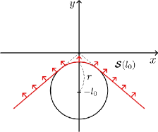
Figure 4: The illustration of $\bm{\mathcal{S}}(l_{0})$.

Lemma 5.

Under the Lévy flight model, the function $H(k,l_{0})$ in (12) has the following characteristics:
(i) Let $\Delta\bm{V}$ be a generic random variable for $\bm{V}_{i}(k)-\bm{V}_{j}(k)$ representing a flight differential between nodes $i$ and $j$. Then, geometrically the function $H(1,l_{0})$ can be viewed as the probability of the flight differential falling into a set $\bm{\mathcal{S}}(l_{0})\,(\subset\mathbb{R}^{2})$ defined as follows. Let $\bm{\mathcal{D}}_{r}(\bm{u})\,(\subset\mathbb{R}^{2})$ denote a disc of radius $r$ centered at $\bm{u}\in\mathbb{R}^{2}$, i.e., $\bm{\mathcal{D}}_{r}(\bm{u})\triangleq\{\bm{x}\in\mathbb{R}^{2}\,|\,|\bm{x}-\bm{u}|\leq r\}$. Let $\overline{(\bm{v},\bm{w})}$ denote a line connecting two points $\bm{v},\bm{w}\in\mathbb{R}^{2}$. For a fixed $l_{0}\in(r,2\sqrt{n}]$, define a set $\bm{\mathcal{S}}(l_{0})$ as

$$\bm{\mathcal{S}}(l_{0}) \triangleq\big{\{}\bm{x}\in\mathbb{R}^{2}\,\big{|}\,\overline{(\bm{0},\bm{x})}\cap\bm{\mathcal{D}}_{r}((0,-l_{0}))=\varnothing\big{\}}.$$ (17)

An example of $\bm{\mathcal{S}}(l_{0})$ is shown in Fig. 4. The set $\bm{\mathcal{S}}(l_{0})$ has a connection with the function $H(1,l_{0})$ as follows:

$$H(1,l_{0}) =\text{P}\big{\{}\Delta\bm{V}\in\bm{\mathcal{S}}(l_{0})\big{\}}.$$

(ii) The function $H(1,\cdot)$ is nondecreasing.
(iii) From (ii), we have $H(1,l_{0})\leq\hat{P}$ for all $l_{0}\in(r,2\sqrt{n}]$, where

$$\hat{P}\triangleq H(1,2\sqrt{n}).$$ (18)

(iv) For $k=2,3,\ldots$, each function $H(k,l_{0})$ is also bounded above by $\hat{P}$. Thus, for all $k\in\mathbb{N}$ and $l_{0}\in(r,2\sqrt{n}]$, we have

$$H(k,l_{0}) \leq\hat{P}.$$

(v) There exist constants $c_{l},c_{u}\,(>0)$, and $n_{\text{th}}\in\mathbb{N}$ such that for all $n\geq n_{\text{th}}$, $\hat{P}$ is bounded above and below by

$$\hat{P} \leq 1-\frac{2c_{l}}{\pi}\left(\frac{1}{2\sqrt{n}+r}\right)^{\alpha}\sin^{-1}\left(\frac{r}{2\sqrt{n}}\right),$$ (19a)

$$\hat{P} \geq 1-\frac{2^{\alpha/2+2}c_{u}}{\pi}\left(\frac{1}{2\sqrt{n}-r}\right)^{\alpha}\sin^{-1}\left(\frac{r}{2\sqrt{n}}\right).$$ (19b)

Proof: See Appendix B. $\blacksquare$

Based on the formula for $\text{P}\{T>\tau\}$ in Lemma 2 and (iv) in Lemma 5, we derive a bound on $\text{P}\{T>\tau\}$ in terms of $\hat{P}$ as follows: for $\tau=1,2,\ldots$, we have from (iv) in Lemma 5 that

$$0\leq\prod_{k=1}^{\tau}H(k,l_{0})\leq(\hat{P})^{\tau}.$$ (20)

Since (20) holds for all $l_{0}\in(r,2\sqrt{n}]$, by integrating (20) over $l_{0}\in(r,2\sqrt{n}]$, we have

$$\int_{r^{+}}^{2\sqrt{n}}\Big{(}\prod_{k=1}^{\tau}H(k,l_{0})\Big{)}\,\text{d}F_{L(0)}(l_{0})$$

$$\quad\leq\int_{r^{+}}^{2\sqrt{n}}(\hat{P})^{\tau}\,\text{d}F_{L(0)}(l_{0})=(\hat{P})^{\tau}P_{o}.$$ (21)

By combining (V) and Lemma 2, we have

$$\text{P}\{T>\tau\} \leq(\hat{P})^{\tau}P_{o},\quad\text{ for }\tau=1,2,\ldots.$$ (22)

Since $\text{P}\{T>\tau\}=P_{o}$ for $\tau=0$, the bound in (22) also holds for $\tau=0$. The above result is summarized in Lemma 6.

Lemma 6.

Under the Lévy flight model, the CCDF of the first meeting time $T$ is bounded by

$$\text{P}\{T>\tau\} \leq(\hat{P})^{\tau}P_{o},\quad\text{ for }\tau=0,1,\ldots,$$

where $\hat{P}$ and $P_{o}$ are defined in (18) and (14), respectively.

Proof: Combining Lemma 2 and (iv) in Lemma 5 gives Lemma 6. The detailed derivation was described earlier in (20)-(22). $\blacksquare$

Lemma 7.

The expectation $\text{E}[\lceil T\rceil]$ under the Lévy flight model is bounded by

$$\text{E}\big{[}\lceil T\rceil\big{]}\leq\frac{P_{o}}{1-\hat{P}}.$$

Proof: Using Lemma 6, we can give a bound on $\text{E}[\lceil T\rceil]$ in Lemma 4 as

$$\text{E}\big{[}\lceil T\rceil\big{]}=\sum_{\tau=0}^{\infty}\text{P}\{T>\tau\}\leq P_{o}\sum_{\tau=0}^{\infty}(\hat{P})^{\tau}.$$

By (v) in Lemma 5, we have $\hat{P}<1$ for any $r>0$. Thus, the expectation $\text{E}[\lceil T\rceil]$ is bounded by the geometric series which converges to $\frac{P_{o}}{1-\hat{P}}$. $\blacksquare$

Step 3 (Analysis of the delay scaling): In Lemma 1, we have analyzed the order of the per-node throughput $\lambda_{\hat{\pi}}$ of the scheme $\hat{\pi}$. The results in Lemma 4, (v) in Lemma 5, and Lemma 7 allow us to analyze the order of the average delay $\bar{D}_{\hat{\pi}}$, which is shown in Lemma 8.

Lemma 8.

Let the communication range $r$ scale as $\Theta(n^{\beta})$ $(0\leq\beta\leq 1/4)$. Then, the average delay $\bar{D}_{\hat{\pi}}$ of the scheme $\hat{\pi}$ under the Lévy flight model with parameter $\alpha\in(0,2]$ scales as follows:

$$\bar{D}_{\hat{\pi}} =O(\min(n^{(1+\alpha)/2-\beta},n)).$$

Proof: Here, we provide a sketch of the proof with details given in Appendix B. Under the Lévy flight model with parameter $\alpha\in(0,2]$, we have $(1-\hat{P})^{-1}=\Theta(n^{(1+\alpha)/2-\beta})$ by (v) in Lemma 5. In addition, $P_{o}=\Theta(1)$ by Lemma 3. Hence, from Lemma 4 and Lemma 7, we have

$$\bar{D}_{\hat{\pi}}\leq\text{E}\big{[}\lceil T\rceil\big{]}\leq\frac{P_{o}}{1-\hat{P}}=\Theta(n^{(1+\alpha)/2-\beta}).$$ (23)

In addition, under the Lévy flight model, we have a trivial upper bound for all $\alpha\in(0,2]$ as

$$\bar{D}_{\hat{\pi}}=O(n).$$ (24)

Combining (23) and (24) yields our lemma. $\blacksquare$

Step 4 (Analysis of the delay-capacity tradeoff): In the last step, we derive the delay-capacity tradeoff under the Lévy flight model. By combining the capacity scaling in Lemma 1 and the delay scaling in Lemma 8, we get the following theorem.

Theorem 1.

Under the Lévy flight model with parameter $\alpha\in(0,2]$, the delay-capacity tradeoff $\bar{D}(\lambda)$ for per-node throughput $\lambda=\Theta(n^{-\eta})~{}(0\leq\eta\leq 1/2)$ is given by

$$\bar{D}(\lambda)=O(\sqrt{\min(n^{1+\alpha}\lambda,n^{2})}).$$

Proof: With the use of $\beta=-\log_{n}\sqrt{\lambda}$, the scheme $\hat{\pi}$ can achieve the per-node throughput $\lambda_{\hat{\pi}}=\lambda$ and the average delay $\bar{D}_{\hat{\pi}}=O(\sqrt{\min(n^{1+\alpha}\lambda,n^{2})})$ by Lemma 1 and Lemma 8, respectively. Therefore, from (10), we have our theorem. $\blacksquare$

VI Delay Analysis for the i.i.d. Mobility Model

In this section, we provide detailed analytical steps for obtaining the optimal delay under the i.i.d. mobility model. We again follow the four steps analogous to those used for the Lévy flight model.

Step 1 (Formulation of the average delay using the first meeting time distribution): From (IV-A), the average delay $\bar{D}_{\hat{\pi}}$ under the scheme $\hat{\pi}$ is obtained by

$$\bar{D}_{\hat{\pi}} =\text{P}\{d\!\notin\!\mathcal{I}(s)\}\!\cdot\!\text{E}\big{[}\!\min\!\big{(}T_{(i,d)};i\in\mathcal{I}(s)\big{)}\big{|}\,d\notin\mathcal{I}(s)\big{]}.$$ (25)

As pointed out in Step 1 of Section V, the random variables $T_{(i,d)}$ for $i\in\mathcal{I}(s)$ are dependent. However, the dependency disappears when the nodes move to the next locations after a single time slot under the i.i.d. mobility model. The property of choosing a completely independent location at every time slot in the i.i.d. mobility enables this independence to occur. By applying this observation, we derive a bound on $T_{(i,d)}$ for $i\in\mathcal{I}(s)$ as follows: let $|\mathcal{I}(s)|$ denote the cardinality of the set $\mathcal{I}(s)$. We condition on the values of $|\mathcal{I}(s)|$ and rewrite the expectation on the right-hand side of (25) as

$$\begin{split}&\text{E}\big{[}\min\big{(}T_{(i,d)};i\in\mathcal{I}(s)\big{)}\,\big{|}\,d\notin\mathcal{I}(s)\big{]}\\ &=\sum_{m=1}^{n-1}\text{P}\{|\mathcal{I}(s)|=m\,|\,d\notin\mathcal{I}(s)\}\\ &\qquad\quad\cdot\text{E}\big{[}\min\big{(}T_{(i,d)};i\in\mathcal{I}(s)\big{)}\,\big{|}\,|\mathcal{I}(s)|=m,d\notin\mathcal{I}(s)\big{]}\\ &=\sum_{m=1}^{n-1}\text{P}\{|\mathcal{I}(s)|=m\,|\,d\notin\mathcal{I}(s)\}\cdot\text{E}\big{[}\min\big{(}T^{\star}_{1},T^{\star}_{2},\ldots,T^{\star}_{m}\big{)}\big{]},\end{split}$$ (26)

where $T^{\star}_{v}\,(v=1,\ldots,m)$ denotes the first meeting time of the node $d$ and the $v$th node in the set $\mathcal{I}(s)$, provided that $|\mathcal{I}(s)|=m$ and $d\notin\mathcal{I}(s)$. Let $T_{1},\ldots,T_{m}$ be $m$ independent copies of the generic random variable $T$. Then, we can derive a bound on $T^{\star}_{v}$ in terms of $T_{v}$ as follows:

$$T_{v}^{\star} \triangleq\inf\{t\geq 0\,|\,L_{(i_{v},d)}(t)\leq r,i_{v}\in\mathcal{I}(s),d\notin\mathcal{I}(s)\}$$

$$\leq\inf\{t\geq 1\,|\,L_{(i_{v},d)}(t)\leq r,i_{v}\in\mathcal{I}(s),d\notin\mathcal{I}(s)\}$$

$$\stackrel{{\scriptstyle\text{d}}}{{=}}1+T_{v}.$$ (27)

Here, $i_{v}$ denotes the $v$th index in the set $\mathcal{I}(s)$ and $\stackrel{{\scriptstyle\text{d}}}{{=}}$ denotes “equal in distribution”. The last equation comes from the aforementioned nature of the i.i.d. mobility model in which the locations of nodes are reshuffled at every time slot.

We define a function $\bar{U}:\{1,2,\ldots,n-1\}\to\mathbb{R}$ by

$$\bar{U}(m)\triangleq\text{E}\big{[}\min\big{(}\lceil T_{v}\rceil;v=1,\ldots,m\big{)}\big{]}.$$ (28)

Note that discretization of a random variable $T_{v}$ to $\lceil T_{v}\rceil$ is for mathematical simplicity and it does not affect the result (i.e., order of the optimal delay) of this paper. The function $\bar{U}(m)$ works as a tight upper bound on $\bar{D}_{\hat{\pi}}$ as shown in the following lemma.

Lemma 9.

The average delay $\bar{D}_{\hat{\pi}}$ of the scheme $\hat{\pi}$ under the i.i.d. mobility model is bounded by

$$\bar{D}_{\hat{\pi}} \leq P_{o}+P_{o}\cdot\text{E}\big{[}\bar{U}(B_{(n-2,P_{o}^{c})}+1)\big{]},$$ (29)

where $P_{o}$ is defined in (14), $P_{o}^{c}\triangleq 1-P_{o}$, and $B_{(n-2,P_{o}^{c})}$ denotes a binomial random variable with parameters $n-2$ (trial) and $P_{o}^{c}$ (probability). The function $\bar{U}(m)\,(m=1,\ldots,n-1)$ can be obtained from the distribution of $T$ by

$$\bar{U}(m)=\sum_{\tau=0}^{\infty}\big{(}\text{P}\{T>\tau\}\big{)}^{m}.$$

Proof: Since $T_{v}^{\star}\leq 1+T_{v}\leq 1+\lceil T_{v}\rceil$ for $v=1,\ldots,m$ by (VI), we have

$$\min\big{(}T_{1}^{\star},\ldots,T_{m}^{\star}\big{)} \leq 1+\min\big{(}\lceil T_{1}\rceil,\ldots,\lceil T_{m}\rceil\big{)}.$$

By taking expectations, we have

$$\text{E}\big{[}\min\big{(}T_{1}^{\star},\ldots,T_{m}^{\star}\big{)}\big{]} \leq 1+\bar{U}(m).$$ (30)

Since $\bm{X}_{i}(0)$ is independent and identically distributed across node index $i$, each node $i\,(\neq s)$ belongs to the set $\mathcal{I}(s)$ independently of each other with probability $P_{o}^{c}$. Thus, the random variable $|\mathcal{I}(s)|-1$ (here, 1 is subtracted to exclude the case $s\in\mathcal{I}(s)$) subjected to the condition $d\notin\mathcal{I}(s)$ follows a binomial distribution with parameters $n-2$ and $P_{o}^{c}$, i.e.,

$$\text{P}\{|\mathcal{I}(s)|=m\,|\,d\notin\mathcal{I}(s)\}=\text{P}\{B_{(n-2,P_{o}^{c})}=m-1\}.$$ (31)

By applying (30) and (31) to (26), we have

$$\text{E}\big{[}\min\big{(}T_{(i,d)};i\in\mathcal{I}(s)\big{)}\,\big{|}\,d\notin\mathcal{I}(s)\big{]}$$

$$\quad\leq 1+\text{E}\big{[}\bar{U}(B_{(n-2,P_{o}^{c})}+1)\big{]}.$$ (32)

Combining (25) and (VI) yields (29).

Since the random variable $\min(\lceil T_{v}\rceil;v=1,\ldots,m)$ takes on only nonnegative integer values, $\bar{U}(m)$ can be obtained by

$$\bar{U}(m)=\sum_{\hat{\tau}=1}^{\infty}\text{P}\big{\{}\min\big{(}\lceil T_{v}\rceil;v=1,\ldots,m\big{)}\geq\hat{\tau}\big{\}}.$$ (33)

By noting that $\lceil T_{v}\rceil$ is independent and identically distributed across $v=1,\ldots,m$, we have

$$\text{P}\big{\{}\min\big{(}\lceil T_{v}\rceil;v=1,\ldots,m\big{)}\geq\hat{\tau}\big{\}}$$

$$\quad=\big{(}\text{P}\big{\{}\lceil T\rceil\geq\hat{\tau}\big{\}}\big{)}^{m}=\big{(}\text{P}\big{\{}T>\hat{\tau}-1\big{\}}\big{)}^{m},$$ (34)

where the second equality comes from the property that $\text{P}\{\lceil T\rceil\geq\hat{\tau}\}=\text{P}\{T>\hat{\tau}-1\}$ for all $\hat{\tau}=1,2,\ldots$. Hence, applying (VI) to (33) and replacing $\hat{\tau}-1$ with $\tau$ give the lemma. $\blacksquare$

Step 2 (Characterization of the first meeting time distribution): In this step, similarly to the approach for the Lévy flight model, we first analyze the characteristics of the function $H(k,l_{0})$ in (12) under the i.i.d. mobility model (See Lemma 10). By exploiting the characteristics, we then derive a bound on the first meeting time distribution (See Lemma 11). This bound enables us to derive a formula for the function $\bar{U}(\cdot)$ used in Lemma 9 (See Lemma 12).

As will be shown below, the characteristics of $H(k,l_{0})$ under the i.i.d. mobility model are similar to those under the Lévy flight model. Hence, an upper bound on $\text{P}\{T>\tau\}$ can be derived using the probabilities $\hat{P}\,(\triangleq H(1,2\sqrt{n}))$ and $P_{o}$ also for the i.i.d. mobility model. The main difference is that the formula for $H(1,l_{0})$ is of different form and has a different scaling property when $l_{0}=2\sqrt{n}$.

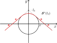
Figure 5: The illustration of $\bm{\mathcal{S}}^{\star}(l_{0})$.

Lemma 10.

Under the i.i.d. mobility model, the function $H(k,l_{0})$ in (12) has the following characteristics:
(i) Let $\Delta\bm{X}$ be a generic random variable for $\bm{X}_{i}(t)-\bm{X}_{j}(t)$ representing a location differential between nodes $i$ and $j$. Then, geometrically the function $H(1,l_{0})$ can be viewed as the probability of the location differential falling into a set $\bm{\mathcal{S}}^{\star}(l_{0})\,(\subset\mathbb{R}^{2})$ defined for $l_{0}\in(r,2\sqrt{n}]$ as

$$\bm{\mathcal{S}}^{\star}(l_{0}) \triangleq\big{\{}\bm{x}\in\mathbb{R}^{2}\,\big{|}\,\overline{((0,l_{0}),\bm{x})}\cap\bm{\mathcal{D}}_{r}(\bm{0})=\varnothing\big{\}},$$ (35)

where the definitions of $\overline{(\cdot,\cdot)}$ and $\bm{\mathcal{D}}_{\cdot}(\cdot)$ can be found in Lemma 5. An example of $\bm{\mathcal{S}}^{\star}(l_{0})$ is shown in Fig. 5. The set $\bm{\mathcal{S}}^{\star}(l_{0})$ has a connection with the function $H(1,l_{0})$ as follows:

$$H(1,l_{0}) =\text{P}\big{\{}\Delta\bm{X}\in\bm{\mathcal{S}}^{\star}(l_{0})\big{\}}.$$

(ii) The function $H(1,\cdot)$ is nondecreasing.
(iii) From (ii), we have $H(1,l_{0})\leq\hat{P}$ for all $l_{0}\in(r,2\sqrt{n}]$.
(iv) For $k=2,3,\ldots$, each function $H(k,l_{0})$ is also bounded above by $\hat{P}$. Thus, for all $k\in\mathbb{N}$ and $l_{0}\in(r,2\sqrt{n}]$, we have

$$H(k,l_{0})\leq\hat{P}.$$

(v) $\hat{P}$ is bounded above and below for all $n\in\mathbb{N}$ by

$$\hat{P} \leq 1-\frac{1}{\pi}\sin^{-1}\Big{(}\frac{r}{2\sqrt{n}}\Big{)},$$ (36a)

$$\hat{P} \geq 1-\frac{r^{2}}{2n}-\frac{2r}{\pi\sqrt{n}}-\frac{5}{\pi}\sin^{-1}\Big{(}\frac{r}{2\sqrt{n}}\Big{)}.$$ (36b)

Proof: See Appendix C. $\blacksquare$

Similarly to Step 2 in Section V, we derive a bound on $\text{P}\{T>\tau\}$ in terms of $\hat{P}$ as follows: from (iv) in Lemma 10 and Lemma 2, we have

$$\text{P}\{T>\tau\} \leq(\hat{P})^{\tau}P_{o},\quad\text{ for }\tau=1,2,\ldots.$$ (37)

Since $\text{P}\{T>\tau\}=P_{o}$ for $\tau=0$, the bound in (37) also holds for $\tau=0$. The above result is summarized in Lemma 11.

Lemma 11.

Under the i.i.d. mobility model, the CCDF of the first meeting time $T$ is bounded by

$$\text{P}\{T>\tau\}\leq(\hat{P})^{\tau}P_{o},\quad\text{ for }\tau=0,1,\ldots,$$

where $\hat{P}$ and $P_{o}$ are defined in (18) and (14), respectively.

Proof: Combining Lemma 2 and (iv) in Lemma 10 gives Lemma 11. The detailed derivation was described earlier in (37). $\blacksquare$

Using Lemma 11, we can give a bound on the function $\bar{U}(m)$ in Lemma 9 as

$$\bar{U}(m)=\sum_{\tau=0}^{\infty}(\text{P}\{T>\tau\})^{m}\leq(P_{o})^{m}\sum_{\tau=0}^{\infty}((\hat{P})^{m})^{\tau}.$$ (38)

By (v) in Lemma 10, we have $(\hat{P})^{m}<1$ for any $r>0$. Thus, $\bar{U}(m)$ is bounded by a convergent geometric series and we summarize the result in Lemma 12.

Lemma 12.

The function $\bar{U}(m)\,(m=1,\ldots,n-1)$ defined in (28) is bounded under the i.i.d. mobility model by

$$\bar{U}(m)\leq\frac{(P_{o})^{m}}{1-(\hat{P})^{m}}.$$

Proof: Combining Lemma 9, (v) in Lemma 10, and Lemma 11 gives Lemma 12. The detailed derivation was described earlier in (38). $\blacksquare$

The bound in Lemma 12 is essentially the same format with that of the slotted contact model under the i.i.d. mobility model. The only difference is that $\hat{P}$ additionally considers intermediate meetings.

Step 3 (Analysis of the delay scaling): In this step, we analyze the order of the average delay $\bar{D}_{\hat{\pi}}$ under the i.i.d. mobility model. To efficiently handle the expectation $\text{E}[\bar{U}(B_{(n-2,P_{o}^{c})}+1)]$ in Lemma 9, we derive a bound on the expectation as follows: first, we rewrite $\text{E}[\bar{U}(B_{(n-2,P_{o}^{c})}+1)]$ by conditioning on $B_{(n-2,P_{o}^{c})}$ as

$$\text{E}[\bar{U}(B_{(\!n\!-\!2,P_{o}^{c})}\!+\!1)]\!=\!\sum_{m=1}^{n-1}\bar{U}(m)\!\cdot\!\text{P}\{B_{(\!n\!-\!2,P_{o}^{c})}\!=\!m\!-\!1\}.$$ (39)

We then decompose (39) into two terms as

$$\text{E}\big{[}\bar{U}(B_{(n-2,P_{o}^{c})}+1)\big{]}$$

$$=\sum_{m=1}^{\lceil\gamma r^{2}\rceil-1}\bar{U}(m)\cdot\text{P}\{B_{(n-2,P_{o}^{c})}=m-1\}$$

$$\qquad+\sum_{m=\lceil\gamma r^{2}\rceil}^{n-1}\bar{U}(m)\cdot\text{P}\{B_{(n-2,P_{o}^{c})}=m-1\}$$

$$\leq\bar{U}(1)\sum_{m=1}^{\lceil\gamma r^{2}\rceil-1}\text{P}\{B_{(n-2,P_{o}^{c})}=m-1\}+\bar{U}(\lceil\gamma r^{2}\rceil),$$ (40)

where $\gamma$ is a constant in $(0,1)$ and $\gamma r^{2}$ implies the $\gamma$ fraction of the average number of nodes within the communication range of a source node. In (VI), we used the property that $\bar{U}(m)$ is a nonincreasing function of $m$. Hence, by Lemma 9 and (VI), the average delay $\bar{D}_{\hat{\pi}}$ of the scheme $\hat{\pi}$ under the i.i.d. mobility model is bounded by:

$$\bar{D}_{\hat{\pi}} \leq P_{o}+P_{o}\cdot\bar{U}(1)\cdot\text{P}\{B_{(n-2,P_{o}^{c})}\leq\lceil\gamma r^{2}\rceil-2\}$$

$$\qquad+P_{o}\cdot\bar{U}(\lceil\gamma r^{2}\rceil).$$ (41)

The results in (VI), Lemmas 3 and 12, and (v) in Lemma 10 allow us to analyze the order of the average delay $\bar{D}_{\hat{\pi}}$, which is shown in Lemma 13.

Lemma 13.

Let the communication range $r$ scale as $\Theta(n^{\beta})$ $(0\leq\beta\leq 1/4)$. Then, the average delay $\bar{D}_{\hat{\pi}}$ of the scheme $\hat{\pi}$ under the i.i.d. mobility model scales as follows:

$$\bar{D}_{\hat{\pi}} =O(n^{\max(0,1/2-3\beta)}).$$

Proof: Here, we provide a sketch of the proof with details given in Appendix C.
Order of $P_{o}$: By Lemma 3,

$$P_{o}=\Theta(1).$$ (42)

Order of $\bar{U}(1)$: By (v) in Lemma 10, we have $(1-\hat{P})^{-1}=\Theta(n^{1/2-\beta})$. Hence, combining (42) and Lemma 12 yields

$$\bar{U}(1)\leq\frac{P_{o}}{1-\hat{P}}=\Theta(n^{1/2-\beta}).$$ (43)

Order of $\bar{U}(\lceil\gamma r^{2}\rceil)$: By (42), we have $(P_{o})^{\lceil\gamma r^{2}\rceil}=\Theta(1)$. In addition, by (v) in Lemma 10, we have $(1-(\hat{P})^{\lceil\gamma r^{2}\rceil})^{-1}=\Theta(n^{\max(0,1/2-3\beta)})$. Hence, Lemma 12 gives

$$\bar{U}(\lceil\gamma r^{2}\rceil)\leq\frac{(P_{o})^{\lceil\gamma r^{2}\rceil}}{1-(\hat{P})^{\lceil\gamma r^{2}\rceil}}=\Theta(n^{\max(0,1/2-3\beta)}).$$ (44)

Order of $\text{P}\{B_{(n-2,P_{o}^{c})}\leq\lceil\gamma r^{2}\rceil-2\}$: By using Chernoff’s inequality, for any fixed $\gamma\in(0,1/3)$ and $n\geq\frac{2}{1-3\gamma}$, we have

$$\text{P}\{B_{(n-2,P_{o}^{c})}\leq\gamma r^{2}\} \leq\exp\left(-\frac{1}{2}\Big{(}\frac{n-2-3\gamma n}{3n}\Big{)}^{2}r^{2}\right)$$

$$\leq 2\Big{(}\frac{3n}{n-2-3\gamma n}\Big{)}^{2}r^{-2}=O(n^{-2\beta}),$$

which results in

$$\text{P}\{B_{(n-2,P_{o}^{c})}\leq\lceil\gamma r^{2}\rceil-2\} =O(n^{-2\beta}).$$ (45)

Combining (VI)-(45) gives the lemma. $\blacksquare$

Step 4 (Analysis of the delay-capacity tradeoff): In the last step, we derive the delay-capacity tradeoff under the i.i.d. mobility model. By combining the capacity scaling in Lemma 1 and the delay scaling in Lemma 13, we get the following theorem.

Theorem 2.

Under the i.i.d. mobility model, the delay-capacity tradeoff $\bar{D}(\lambda)$ for per-node throughput $\lambda=\Theta(n^{-\eta})~{}(0\leq\eta\leq 1/2)$ is given by

$$\bar{D}(\lambda) =O(\sqrt{\max(1,n\lambda^{3})}).$$

Proof: With the use of $\beta=-\log_{n}\sqrt{\lambda}$, the scheme $\hat{\pi}$ can achieve the per-node throughput $\lambda_{\hat{\pi}}=\lambda$ and the average delay $\bar{D}_{\hat{\pi}}=O(\sqrt{\max(1,n\lambda^{3})})$ by Lemma 1 and Lemma 13, respectively. Therefore, from (10), we have our theorem. $\blacksquare$

VII Concluding Remarks

In this paper, we developed a new analytical framework that substantially improves the realism in delay-capacity analysis by considering (i) Lévy flight mobility, which is known to closely resemble human mobility patterns and (ii) contact opportunities in the middle of movements of nodes. Using our framework, we obtained the first delay-capacity tradeoff for Lévy flight and derived a new tighter tradeoff for i.i.d. mobility. For Lévy flight, our analysis shows that the tradeoff holds $\bar{D}(\lambda)=O(\sqrt{\min(n^{1+\alpha}\lambda,n^{2})})$ for $\lambda=\Theta(n^{-\eta})\,(0\leq\eta\leq 1/2)$ as shown in Figs. 2 (a), 3 (a), and  3 (b). Our result is well aligned with the critical delay suggested in [13]. For i.i.d. mobility, our analysis provides $\bar{D}(\lambda)=O(\sqrt{\max(1,n\lambda^{3})})$ as shown in Fig. 2 (b). These tradeoffs are especially remarkable in both Lévy flight and i.i.d. mobility for the constant per-node throughput (i.e., $\lambda=\Theta(1)$) as they demonstrate that the delay can be less than $\Theta(n)$, which has been widely accepted for most mobility models. Our future work includes (i) an extension of our framework to analyze the delay-capacity tradeoff under Lévy walk and (ii) another extension to capture correlated movement patterns among nodes.

Appendix A Proof of Lemma 3

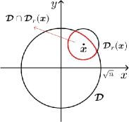
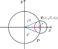
Figure 6: Examples of $\bm{\mathcal{D}}\cap\bm{\mathcal{D}}_{r}(\bm{x})$: $\text{Area}(\bm{\mathcal{D}}\cap\bm{\mathcal{D}}_{r}(\bm{x}))$ is nonincreasing as $|\bm{x}|$ increases (Left). When $|\bm{x}|=n$ (e.g., $\bm{x}=(\sqrt{n},0)$), $\text{Area}(\bm{\mathcal{D}}\cap\bm{\mathcal{D}}_{r}(\bm{x}))$ is minimized and a lower bound on $\text{Area}(\bm{\mathcal{D}}\cap\bm{\mathcal{D}}_{r}((\sqrt{n},0))$ can be obtained in terms of $\theta=2\cos^{-1}(\frac{r}{2\sqrt{n}})$, as given in (A) (Right).

By the definition of $P_{o}$ in (14), we have

$$P_{o} =\text{P}\{L_{(i,j)}(0)>r\}=1-\text{P}\{L_{(i,j)}(0)\leq r\}.$$ (46)

Let $F_{\bm{X}_{i}(0)}(\cdot)$ denote the CDF of $\bm{X}_{i}(0)$. Then, by conditioning on the values of $\bm{X}_{i}(0)$, the probability $\text{P}\{L_{(i,j)}(0)\leq r\}$ in (46) can be rewritten as

$$\text{P}\{L_{(i,j)}(0)\leq r\}$$

$$\quad=\int_{\bm{\mathcal{D}}}\text{P}\{L_{(i,j)}(0)\leq r|\bm{X}_{i}(0)=\bm{x}\}\,\text{d}F_{\bm{X}_{i}(0)}(\bm{x})$$

$$\quad=\int_{\bm{\mathcal{D}}}\text{P}\{\bm{X}_{j}(0)\in\bm{\mathcal{D}}_{r}(\bm{x})|\bm{X}_{i}(0)=\bm{x}\}\,\text{d}F_{\bm{X}_{i}(0)}(\bm{x})$$

$$\quad=\int_{\bm{\mathcal{D}}}\text{P}\{\bm{X}_{j}(0)\in\bm{\mathcal{D}}_{r}(\bm{x})\}\,\text{d}F_{\bm{X}_{i}(0)}(\bm{x}),$$ (47)

where the last equality comes from the independence between $\bm{X}_{i}(0)$ and $\bm{X}_{j}(0)$. Note that, since $\bm{X}_{j}(0)\in\bm{\mathcal{D}}$ with probability 1 and $\bm{X}_{j}(0)\sim\text{Uniform}(\bm{\mathcal{D}})$, the probability $\text{P}\{\bm{X}_{j}(0)\in\bm{\mathcal{D}}_{r}(\bm{x})\}$ in the integral in (A) is given by

$$\text{P}\{\bm{X}_{j}(0)\in\bm{\mathcal{D}}_{r}(\bm{x})\}=\frac{\text{Area}(\bm{\mathcal{D}}\cap\bm{\mathcal{D}}_{r}(\bm{x}))}{\text{Area}(\bm{\mathcal{D}})},$$ (48)

where $\text{Area}(\bm{S})$ denotes the area of a set $\bm{S}\subset\mathbb{R}^{2}$. An example of $\bm{\mathcal{D}}\cap\bm{\mathcal{D}}_{r}(\bm{x})$ is shown in Fig. 6. From the figure, it is obvious that $\text{Area}(\bm{\mathcal{D}}\cap\bm{\mathcal{D}}_{r}(\bm{x}))$ is nonincreasing as $\bm{x}$ approaches to the boundary of the disc $\bm{\mathcal{D}}$. Hence, (48) is bounded above by

$$\text{P}\{\bm{X}_{j}(0)\in\bm{\mathcal{D}}_{r}(\bm{x})\} \leq\frac{\text{Area}(\bm{\mathcal{D}}\cap\bm{\mathcal{D}}_{r}(\bm{0}))}{\pi(\sqrt{n})^{2}}$$

$$=\frac{\text{Area}(\bm{\mathcal{D}}_{r}(\bm{0}))}{\pi n}=\frac{r^{2}}{n}.$$ (49)

In addition, it is bounded below by

$$\text{P}\{\bm{X}_{j}(0)\in\bm{\mathcal{D}}_{r}(\bm{x})\} \geq\frac{\text{Area}(\bm{\mathcal{D}}\cap\bm{\mathcal{D}}_{r}((\sqrt{n},0)))}{\pi(\sqrt{n})^{2}}$$

$$\geq\frac{\pi r^{2}}{\pi n}\frac{\theta}{2\pi}=\frac{r^{2}}{n}\frac{\theta}{2\pi},$$ (50)

where $\theta\triangleq 2\cos^{-1}(\frac{r}{2\sqrt{n}})$ (See Fig. 6). Since $\sqrt{n}\geq r$, we have $\theta\geq 2\cos^{-1}(\frac{r}{2r})=\frac{2\pi}{3}$. Hence, the inequality in (A) is further bounded by

$$\text{P}\{\bm{X}_{j}(0)\in\bm{\mathcal{D}}_{r}(\bm{x})\} \geq\frac{r^{2}}{3n}.$$ (51)

By substituting (A) and (51) into (A), we have

$$\frac{r^{2}}{3n}\leq\text{P}\{L_{(i,j)}(0)\leq r\}\leq\frac{r^{2}}{n},$$

which, combined with (46), gives

$$1-\frac{r^{2}}{n}\leq P_{o}\leq 1-\frac{r^{2}}{3n}.$$

Appendix B Proofs of Lemmas for the Lévy Flight Model

Here, we give detailed proofs of Lemmas 5 and 8, which are used for analyzing the optimal delay under the Lévy flight model. To prove Lemma 5, we need the following Lemmas 14, 15, and 16.

Lemma 14.

For $i\neq j$ and $k\in\mathbb{N}$, let

$$\Delta\bm{V}_{(i,j)}(k)\triangleq\bm{V}_{i}(k)-\bm{V}_{j}(k),$$

where $\bm{V}_{\cdot}(k)$ (representing the $k$th flight of a node $\cdot$) is defined in (3). Then, under the Lévy flight model, $\Delta\bm{V}_{(i,j)}(k)$ has the following properties:
(i) $\Delta\bm{V}_{(i,j)}(k)$ is independent of $\bm{X}_{u}(t)$ for all $u=1,\ldots,n$ and $t\in[0,k-1]$.
(ii) $\Delta\bm{V}_{(i,j)}(k)$ is identically distributed across pair index $(i,j)$ and slot index $k$. Hence, we use $\Delta\bm{V}$ to denote a generic random variable for $\Delta\bm{V}_{(i,j)}(k)$.
(iii) For $\bm{v}\in\mathbb{R}^{2}$, let $\angle\bm{v}$ denote the angle at vertex $\bm{0}$ enclosed by the line $\overline{(\bm{0},\bm{v})}$ and the positive $x$-axis. Then, the angle $\angle\Delta\bm{V}$ is a uniform random variable on the interval $(0,2\pi]$ and is independent of the length $|\Delta\bm{V}|$.

Proof: (i) For any $u=1,\ldots,n$, $\bm{X}_{u}(t)\,(0\leq t\leq k-1)$ under the Lévy flight model is completely determined by $\bm{F}_{u}(k-1)\triangleq\{\bm{X}_{u}(0),\bm{V}_{u}(1),\ldots,\bm{V}_{u}(k-1)\}$ (by the relations (1) and (2)). Since $\bm{V}_{i}(k)$ is independent of $\bm{F}_{u}(k-1)$, it is independent of $\bm{X}_{u}(t)$. By the same reason, $\bm{V}_{j}(k)$ is independent of $\bm{X}_{u}(t)$. Therefore, the difference $\bm{V}_{i}(k)-\bm{V}_{j}(k)$ is independent of $\bm{X}_{u}(t)$.
(ii) Since each of the flight angle $\theta_{u}(k)$ and the flight length $Z_{u}(k)$ is independent and identically distributed across node index $u$ and slot index $k$, the random variable $\bm{V}_{u}(k)\,(\triangleq(Z_{u}(k)\cos\theta_{u}(k),Z_{u}(k)\sin\theta_{u}(k)))$ is also independent and identically distributed across $u$ and $k$. Therefore, the difference $\bm{V}_{i}(k)-\bm{V}_{j}(k)$ is identically distributed across pair index $(i,j)$ and slot index $k$. However, it is not necessarily independent across $(i,j)$ while it is independent across $k$ for a fixed $(i,j)$.
(iii) To prove (iii), it suffices to show that for any $v\geq 0$,

$$\text{P}\big{\{}\angle\Delta\bm{V}_{(i,j)}(k)\leq\theta\,\big{|}\,|\Delta\bm{V}_{(i,j)}(k)|=v\big{\}}=\frac{\theta}{2\pi},$$ (52)

where $0<\theta\leq 2\pi$. In the following, we will prove (52).

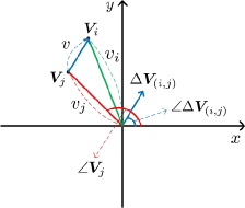
Figure 7: An example of vectors satisfying the condition in (54): for a given $(v_{i},v_{j},v)$, the angle $\angle\Delta\bm{V}_{(i,j)}$ is determined by the angle $\angle\bm{V}_{j}$. Since $\angle\bm{V}_{j}\sim\text{Uniform}[0,2\pi]$, we have $\angle\Delta\bm{V}_{(i,j)}\sim\text{Uniform}[0,2\pi]$.

For simplicity, we omit the slot index $k$ in $\bm{V}_{\cdot}(k)$ and $\Delta\bm{V}_{(i,j)}(k)$ in the rest of this proof. By conditioning on the values of $(|\bm{V}_{i}|,|\bm{V}_{j}|)$, we can rewrite the probability on the left-hand side of (52) as follows:

$$\text{P}\big{\{}\angle\Delta\bm{V}_{(i,j)}\leq\theta\,\big{|}\,|\Delta\bm{V}_{(i,j)}|=v\big{\}}$$

$$=\int_{(v_{i},v_{j})}\!\!\!\text{P}\big{\{}\angle\Delta\bm{V}_{(i,j)}\leq\theta\big{|}(|\bm{V}_{i}|,|\bm{V}_{j}|,|\Delta\bm{V}_{(i,j)}|)\!=\!(v_{i},v_{j},v)\big{\}}$$

$$\hskip 34.1433pt\cdot\text{P}\big{\{}(|\bm{V}_{i}|,|\bm{V}_{j}|)\!=\!(v_{i},v_{j})\big{|}|\Delta\bm{V}_{(i,j)}|\!=\!v\big{\}}\,\text{d}(v_{i},v_{j}).$$ (53)

For a fixed $v\geq 0$, consider an event $\{(|\bm{V}_{i}|,|\bm{V}_{j}|)=(v_{i},v_{j})\}$ such that

$$\text{P}\big{\{}(|\bm{V}_{i}|,|\bm{V}_{j}|)=(v_{i},v_{j})\,\big{|}\,|\Delta\bm{V}_{(i,j)}|=v\big{\}}>0.$$ (54)

An example satisfying (54) is shown in Fig. 7. Under the condition $(|\bm{V}_{i}|,|\bm{V}_{j}|,|\Delta\bm{V}_{(i,j)}|)=(v_{i},v_{j},v)$, the angle $\angle\Delta\bm{V}_{(i,j)}$ is determined by the angle $\angle\bm{V}_{j}$ as the figure shows. Since $\angle\bm{V}_{j}\sim\text{Uniform}[0,2\pi]$, we have $\angle\Delta\bm{V}_{(i,j)}\sim\text{Uniform}[0,2\pi]$. That is, for $0<\theta\leq 2\pi$ we have

$$\text{P}\big{\{}\angle\Delta\bm{V}_{(i,j)}\leq\theta\,\big{|}\,(|\bm{V}_{i}|,|\bm{V}_{j}|,|\Delta\bm{V}_{(i,j)}|)=(v_{i},v_{j},v)\big{\}}=\frac{\theta}{2\pi}.$$

Since the above equality holds for any $(v_{i},v_{j})$ satisfying (54) for a given $v$, the probability in (B) boils down to the following:

$$\text{P}\big{\{}\angle\Delta\bm{V}_{(i,j)}\leq\theta\,\big{|}\,|\Delta\bm{V}_{(i,j)}|=v\big{\}}$$

$$=\frac{\theta}{2\pi}\int_{(v_{i},v_{j})}\!\!\!\text{P}\big{\{}(|\bm{V}_{i}|,|\bm{V}_{j}|)\!=\!(v_{i},v_{j})\,\big{|}\,|\Delta\bm{V}_{(i,j)}|\!=\!v\big{\}}\,\text{d}(v_{i},v_{j})$$

$$=\frac{\theta}{2\pi}.$$

This completes the proof. $\blacksquare$

Lemma 15.

Suppose $k\in\mathbb{N}$ and $l\in(r,2\sqrt{n}]$. Then, for any sets $\mathcal{L}(\cdot)\subset[0,2\sqrt{n}]$ satisfying

$$\text{P}\{L(k-1)=l,L(t)\in\mathcal{L}(t),0\leq t\leq k-1\}>0,$$ (55)

we have under the Lévy flight model the following:

$$\text{P}\{I(k)=0\,|\,L(k-1)=l,L(t)\in\mathcal{L}(t),0\leq t\leq k-1\}$$

$$\quad=\text{P}\{\Delta\bm{V}\in\bm{\mathcal{S}}(l)\}.$$ (56)

The definitions of $\Delta\bm{V}$ and $\bm{\mathcal{S}}(l)$ can be found in Lemma 5.

Remark 1.

Before proving the lemma, we give a remark. Lemma 15 implies that the future states of a meeting process under the Lévy flight model depend only on the state at the beginning of the current slot, not on the sequence of events that preceded it. In addition, the conditional probability distribution of the future state described above is time homogeneous (i.e., the probability in (15) does not depend on the slot index $k$). This restricted time homogeneous memoryless property enables us to derive a bound on the first meeting time distribution as a geometric form (See Lemma 6).

Proof: For notational simplicity, we let

$$\mathcal{F}(k-1)\triangleq\{L(t)\in\mathcal{L}(t),0\leq t\leq k-1\}$$ (57)

satisfying (55). For $i\neq j$ and $t\geq 0$, let

$$\Delta\bm{X}_{(i,j)}(t)\triangleq\bm{X}_{i}(t)-\bm{X}_{j}(t).$$

For simplicity, we omit $(i,j)$ in $\Delta\bm{X}_{(i,j)}(t)$. Then, by conditioning on the values of $\angle\Delta\bm{X}(k-1)$, the left-hand side of (15) can be rewritten as

$$\text{P}\{I(k)=0|L(k-1)=l,\mathcal{F}(k-1)\}$$

$$=\!\int_{0}^{2\pi}\!\!\text{P}\{I(k)=0|\angle\Delta\bm{X}(k\!-\!1\!)=\theta,L(k\!-\!1\!)=l,\!\mathcal{F}(k\!-\!1\!)\}$$

$$\hskip 31.29802pt\text{d}F_{\angle\Delta\bm{X}(k-1)|L(k-1)=l,\mathcal{F}(k-1)}(\theta),$$ (58)

where $F_{\angle\Delta\bm{X}(k-1)|L(k-1)=l,\mathcal{F}(k-1)}(\cdot)$ denotes the CDF of the random variable $\angle\Delta\bm{X}(k-1)$ conditioned that $L(k-1)=l$ and $\mathcal{F}(k-1)$. Since $L(k-1)=|\Delta\bm{X}(k-1)|$, the joint condition $\angle\Delta\bm{X}(k-1)=\theta$ and $L(k-1)=l$ is equivalent to $\Delta\bm{X}(k-1)=l\bm{e}^{j\theta}$, where $\bm{e}^{j\theta}\triangleq(\cos\theta,\sin\theta)$. Hence, the probability in (B) can be expressed as

$$\text{P}\{I(k)=0\,|\,\angle\Delta\bm{X}(k-1)=\theta,L(k-1)=l,\mathcal{F}(k-1)\}$$

$$\quad=\text{P}\{I(k)=0\,|\,\Delta\bm{X}(k-1)=l\bm{e}^{j\theta},\mathcal{F}(k-1)\}.$$ (59)

The key idea of the proof is to use the following equality: for any $k\in\mathbb{N}$, $l\in(r,2\sqrt{n}]$, $\theta\in(0,2\pi]$, and $\mathcal{F}(k-1)$, we have

$$\begin{split}&\text{P}\{I(k)=0\,|\,\Delta\bm{X}(k-1)=l\bm{e}^{j\theta},\mathcal{F}(k-1)\}\\ &\quad=\text{P}\{\Delta\bm{V}\in\bm{\mathcal{S}}(l)\}.\end{split}$$ (60)

By substituting the combined result of (B) and (60) into (B), we have the lemma.

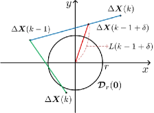
Figure 8: An illustration of a meeting event during the $k$th slot: in case of the blue line, $L(k-1+\delta)>r$ for all $\delta\in(0,1]$, i.e., $I(k)=0$. However, in case of the green line, there exist multiple $\delta\in(0,1]$ such that $L(k-1+\delta)\leq r$, i.e., $I(k)=1$.

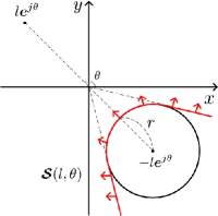
Figure 9: An example of $\bm{\mathcal{S}}(l,\theta)$: when $\theta=\frac{\pi}{2}$, $\bm{\mathcal{S}}(l,\theta)$ is identical to $\bm{\mathcal{S}}(l)$.

In the following, we show (60). We first consider the event $\{I(k)=0\}$. By definition, the event $\{I(k)=0\}$ occurs if and only if $L(t)>r$ for all $t\in(k-1,k]$, equivalently, $L(k-1+\delta)>r$ for all $\delta\in(0,1]$. Since $\bm{X}_{i}(k-1+\delta)=(1-\delta)\bm{X}_{i}(k-1)+\delta\bm{X}_{i}(k)$ by (1), we have

$$\Delta\bm{X}(k-1+\delta)=(1-\delta)\Delta\bm{X}(k-1)+\delta\Delta\bm{X}(k).$$ (61)

This implies that the event $\{L(k-1+\delta)>r~{}\text{for all }\delta\in(0,1]\}$ occurs if and only if the following event occurs (See Fig. 8):

$$\Big{\{}\overline{\big{(}\Delta\bm{X}(k-1),\Delta\bm{X}(k)\big{)}}\cap\bm{\mathcal{D}}_{r}(\bm{0})=\varnothing\Big{\}}.$$ (62)

We next consider the event $\{I(k)=0\}$ conditioned by $\Delta\bm{X}(k-1)=l\bm{e}^{j\theta}$ and $\mathcal{F}(k-1)$. Then, since $\bm{X}_{i}(k)=\bm{X}_{i}(k-1)+\bm{V}_{i}(k)$ by (2), we have

$$\Delta\bm{X}(k) =\Delta\bm{X}(k-1)+\Delta\bm{V}(k)=l\bm{e}^{j\theta}+\Delta\bm{V}(k).$$

Thus, given the conditions $\Delta\bm{X}(k-1)=l\bm{e}^{j\theta}$ and $\mathcal{F}(k-1)$, (62) is reduced to the following:

$$\Big{\{}\overline{\big{(}\Delta\bm{X}(k-1),\Delta\bm{X}(k)\big{)}}\cap\bm{\mathcal{D}}_{r}(\bm{0})=\varnothing\Big{\}}$$

$$\quad=\Big{\{}\overline{\big{(}l\bm{e}^{j\theta},l\bm{e}^{j\theta}+\Delta\bm{V}(k)\big{)}}\cap\bm{\mathcal{D}}_{r}(\bm{0})=\varnothing\Big{\}}$$

$$\quad=\Big{\{}\overline{\big{(}\bm{0},\Delta\bm{V}(k)\big{)}}\cap\bm{\mathcal{D}}_{r}(-l\bm{e}^{j\theta})=\varnothing\Big{\}}$$

$$\quad=\Big{\{}\Delta\bm{V}(k)\in\bm{\mathcal{S}}(l,\theta)\Big{\}},$$

where

$$\bm{\mathcal{S}}(l,\theta)\triangleq\big{\{}\bm{x}\in\mathbb{R}^{2}\,\big{|}\,\overline{(\bm{0},\bm{x})}\cap\bm{\mathcal{D}}_{r}(-l\bm{e}^{j\theta})=\varnothing\big{\}}.$$

An example of $\bm{\mathcal{S}}(l,\theta)$ is shown in Fig. 9. Hence, the probability on the left-hand side of (60) becomes

$$\text{P}\{I(k)=0\,|\,\Delta\bm{X}(k\!-\!1)=l\bm{e}^{j\theta},\mathcal{F}(k\!-\!1)\}$$

$$=\text{P}\{\Delta\bm{V}(k)\in\bm{\mathcal{S}}(l,\theta)\,|\,\Delta\bm{X}(k\!-\!1)=l\bm{e}^{j\theta},\mathcal{F}(k\!-\!1)\}.$$ (63)

By (i) in Lemma 14, $\Delta\bm{V}(k)$ is independent of $\Delta\bm{X}(k-1)$ and $\mathcal{F}(k-1)$, and thus we have

$$\text{P}\{\Delta\bm{V}(k)\in\bm{\mathcal{S}}(l,\theta)\,|\,\Delta\bm{X}(k-1)=l\bm{e}^{j\theta},\mathcal{F}(k-1)\}$$

$$\quad=\text{P}\{\Delta\bm{V}(k)\in\bm{\mathcal{S}}(l,\theta)\}.$$ (64)

In addition, by (ii) in Lemma 14,

$$\text{P}\{\Delta\bm{V}(k)\in\bm{\mathcal{S}}(l,\theta)\}=\text{P}\{\Delta\bm{V}\in\bm{\mathcal{S}}(l,\theta)\}.$$ (65)

Finally, by (iii) in Lemma 14, the probability in (65) is invariant for any $\theta\in(0,2\pi]$. When $\theta=\frac{\pi}{2}$, we have $\bm{\mathcal{S}}(l,\frac{\pi}{2})=\bm{\mathcal{S}}(l)$. Hence, the following holds for any $\theta\in(0,2\pi]$:

$$\text{P}\{\Delta\bm{V}\in\bm{\mathcal{S}}(l,\theta)\}=\text{P}\{\Delta\bm{V}\in\bm{\mathcal{S}}(l)\}.$$ (66)

Combining (B), (B), (65), and (66) gives (60). This completes the proof. $\blacksquare$

Lemma 16.

Let $Z_{1}$, $Z_{2}$ and $\theta_{1},\theta_{2}$ be independent copies of the generic random variables $Z$ (flight length) and $\theta$ (flight angle), respectively. Suppose that there exist constants $c\,(>0)$ and $z_{\text{th}}\,(>0)$ such that

$$\text{P}\{Z>z\}=\frac{c}{z^{\alpha}},\quad\text{ for all }z\geq z_{\text{th}}.$$ (67)

Then, for all $z\geq 2z_{\text{th}}$ we have

$$\frac{c_{l}}{z^{\alpha}}\leq\text{P}\{Z_{1}\cos\theta_{1}-Z_{2}\cos\theta_{2}>z\}\leq\frac{c_{u}}{z^{\alpha}},$$

where

$$c_{l} \triangleq\frac{c}{2\pi}\int_{0}^{\frac{\pi}{2}}(\cos\vartheta)^{\alpha}\,\text{d}\vartheta\,(>0),$$

$$c_{u} \triangleq\frac{2^{1+\alpha}c}{\pi}\int_{0}^{\frac{\pi}{2}}(\cos\vartheta)^{\alpha}\,\text{d}\vartheta\,(>0).$$

Proof: First, we will show that the distribution of $Z\cos\theta$ is of the following power-law form:

$$\text{P}\{Z\cos\theta>x\}=\frac{c_{1}}{x^{\alpha}},\quad\text{ for }x\geq z_{\text{th}},$$ (68)

where $c_{1}\triangleq\frac{c}{\pi}\int_{0}^{\frac{\pi}{2}}(\cos\vartheta)^{\alpha}\,\text{d}\vartheta\,(>0)$. By conditioning on the values of the random variable $\theta\sim\text{Uniform}[0,2\pi]$, the probability $\text{P}\{Z\cos\theta>x\}$ can be rewritten as

$$\text{P}\{Z\cos\theta>x\} =\frac{1}{2\pi}\int_{0}^{2\pi}\text{P}\{Z\cos\vartheta>x\}\,\text{d}\vartheta$$

$$=\frac{1}{\pi}\int_{0}^{\pi}\text{P}\{Z\cos\vartheta>x\}\,\text{d}\vartheta,$$ (69)

where the second equality comes from the symmetry of the function $\cos\vartheta$ with respect to $\vartheta=\pi$. For $x\geq 0$, the integral in (B) can be expressed as

$$\int_{0}^{\pi}\text{P}\{Z\cos\vartheta>x\}\,\text{d}\vartheta$$

$$=\int_{0}^{\frac{\pi}{2}\!-\!\epsilon}\!\!\text{P}\{Z\cos\vartheta>x\}\,\text{d}\vartheta+\int_{\frac{\pi}{2}\!-\!\epsilon}^{\frac{\pi}{2}}\!\!\text{P}\{Z\cos\vartheta>x\}\,\text{d}\vartheta,$$ (70)

where $\epsilon\in(0,\frac{\pi}{2})$. The first integral in (B) becomes

$$\int_{0}^{\frac{\pi}{2}-\epsilon}\text{P}\{Z\cos\vartheta>x\}\,\text{d}\vartheta =\int_{0}^{\frac{\pi}{2}-\epsilon}\text{P}\{Z>\frac{x}{\cos\vartheta}\}\,\text{d}\vartheta$$

$$=\frac{c}{x^{\alpha}}\int_{0}^{\frac{\pi}{2}-\epsilon}(\cos\vartheta)^{\alpha}\,\text{d}\vartheta,$$ (71)

where the first equality comes from $\cos\vartheta>0$ for $\vartheta\in[0,\frac{\pi}{2}-\epsilon]$ and the second equality comes from (67) since $\frac{x}{\cos\vartheta}\geq z_{\text{th}}$ for $x\geq z_{\text{th}}$. The second integral in (B) is bounded by

$$0\leq\int_{\frac{\pi}{2}-\epsilon}^{\frac{\pi}{2}}\text{P}\{Z\cos\vartheta>x\}\,\text{d}\vartheta\leq\int_{\frac{\pi}{2}-\epsilon}^{\frac{\pi}{2}}1\,\text{d}\vartheta=\epsilon.$$ (72)

Combining (B), (B), (B), and (72) gives

$$\frac{c}{\pi x^{\alpha}}\int_{0}^{\frac{\pi}{2}-\epsilon}\!\!(\cos\vartheta)^{\alpha}\,\text{d}\vartheta \leq\text{P}\{Z\cos\theta>x\}$$

$$\leq\frac{c}{\pi x^{\alpha}}\int_{0}^{\frac{\pi}{2}-\epsilon}\!\!(\cos\vartheta)^{\alpha}\,\text{d}\vartheta+\frac{\epsilon}{\pi}.$$ (73)

Letting $\epsilon\to 0$ on (B) yields

$$\text{P}\{Z\cos\theta>x\} =\frac{c}{\pi x^{\alpha}}\int_{0}^{\frac{\pi}{2}}(\cos\vartheta)^{\alpha}\,\text{d}\vartheta.$$

Hence, we have

$$\text{P}\{Z\cos\theta>x\} =\frac{c_{1}}{x^{\alpha}},\quad\text{ for }x\geq z_{\text{th}},$$

where $c_{1}\triangleq\frac{c}{\pi}\int_{0}^{\frac{\pi}{2}}(\cos\vartheta)^{\alpha}\,\text{d}\vartheta\,(>0)$. This proves (68).

In the following, we derive the distribution of the random variable $Z_{1}\cos\theta_{1}-Z_{2}\cos\theta_{2}$ by using (68). Since the event $\{Z_{1}\cos\theta_{1}\leq\frac{z}{2}\}\cap\{Z_{2}\cos\theta_{2}\geq-\frac{z}{2}\}$ implies the event $\{Z_{1}\cos\theta_{1}-Z_{2}\cos\theta_{2}\leq z\}$, we have

$$\text{P}\{Z_{1}\cos\theta_{1}-Z_{2}\cos\theta_{2}>z\}$$

$$\quad\leq\text{P}\{Z_{1}\cos\theta_{1}>\frac{z}{2}\text{ or }Z_{2}\cos\theta_{2}<-\frac{z}{2}\}$$

$$\quad\leq 2\text{P}\{Z\cos\theta>\frac{z}{2}\},$$ (74)

where the last inequality comes from the union bound and the symmetry of $Z\cos\theta$ (i.e., $Z\cos\theta\stackrel{{\scriptstyle\text{d}}}{{=}}-Z\cos\theta$). Suppose $z\geq 2z_{\text{th}}$. Then, by applying (68) to (B), we further have

$$\text{P}\{Z_{1}\cos\theta_{1}-Z_{2}\cos\theta_{2}>z\}\leq\frac{2^{\alpha+1}c_{1}}{z^{\alpha}}=\frac{c_{u}}{z^{\alpha}}.$$ (75)

Similarly, since the event $\{Z_{1}\cos\theta_{1}>z\}\cap\{Z_{2}\cos\theta_{2}<0\}$ implies the event $\{Z_{1}\cos\theta_{1}-Z_{2}\cos\theta_{2}>z\}$, we have

$$\text{P}\{Z_{1}\cos\theta_{1}-Z_{2}\cos\theta_{2}>z\}$$

$$\quad\geq\text{P}\{Z_{1}\cos\theta_{1}>z\text{ and }Z_{2}\cos\theta_{2}<0\}$$

$$\quad=\text{P}\{Z_{1}\cos\theta_{1}>z\}\text{P}\{Z_{2}\cos\theta_{2}<0\}$$

$$\quad=\frac{c_{1}}{2z^{\alpha}}=\frac{c_{l}}{z^{\alpha}},$$ (76)

where the first equality comes from the independence between $Z_{1}\cos\theta_{1}$ and $Z_{2}\cos\theta_{2}$, and the second equality comes from (68) and the symmetry of $Z_{2}\cos\theta_{2}$. Combining (75) and (B) gives the lemma. $\blacksquare$

Proof of Lemma 5

A. Proof of (i)

By choosing $k=1$, $l=l_{0}$, and $\mathcal{L}(0)=(r,2\sqrt{n}]$ in Lemma 15, we have

$$\text{P}\{I(1)=0\,|\,L(0)=l_{0},L(0)\in(r,2\sqrt{n}]\}=\text{P}\{\Delta\bm{V}\in\bm{\mathcal{S}}(l_{0})\}.$$

Since $\{L(0)=l_{0}\}\cap\{L(0)\in(r,2\sqrt{n}]\}=\{L(0)=l_{0}\}$, we further have

$$\text{P}\{I(1)=0\,|\,L(0)=l_{0}\} =\text{P}\{\Delta\bm{V}\in\bm{\mathcal{S}}(l_{0})\}.$$ (77)

By definition, $H(1,l_{0})=\text{P}\{I(1)=0\,|\,L(0)=l_{0}\}$. Thus, we have from (77) that $H(1,l_{0})=\text{P}\{\Delta\bm{V}\in\bm{\mathcal{S}}(l_{0})\}.$

B. Proof of (ii)

Suppose $r<l_{0}\leq l_{1}\leq 2\sqrt{n}$. Then, it is obvious from the definition of $\bm{\mathcal{S}}(\cdot)$ in (17) that $\bm{\mathcal{S}}(l_{0})\subseteq\bm{\mathcal{S}}(l_{1})$ (See Fig. 4). Hence, we have

$$\text{P}\{\Delta\bm{V}\in\bm{\mathcal{S}}(l_{0})\}\leq\text{P}\{\Delta\bm{V}\in\bm{\mathcal{S}}(l_{1})\},$$

which is equivalent to $H(1,l_{0})\leq H(1,l_{1})$ by (i) in Lemma 5.

C. Proof of (iii)

By (ii) in Lemma 5, we have $H(1,l_{0})\leq H(1,2\sqrt{n})\,(=\hat{P})$ for any $l_{0}\in(r,2\sqrt{n}]$.

D. Proof of (iv)

Recall the definition of $H(k,l_{0})$ for $k=2,3,\ldots$:

$$H\!(k,l_{0}\!)\triangleq\text{P}\{I\!(k\!)=0|I\!(k\!-\!1\!)=\ldots=I\!(1\!)=0,L\!(0\!)=l_{0}\}.$$

By conditioning on the values of $L(k-1)$, the probability $H(k,l_{0})$ can be rewritten as

$$H(k,l_{0})$$

$$\!=\!\int_{r^{+}}^{2\sqrt{n}}\!\!\text{P}\{I(k)=0|L(k\!-\!1)=l,I(k\!-\!1)=\ldots=I(1)=0,$$

$$\hskip 36.98857ptL(0)=l_{0}\}\,\text{d}F_{L\!(\!k\!-\!1\!)|I\!(\!k\!-\!1\!)=\ldots=I\!(\!1\!)=0,L\!(\!0\!)=l_{0}}(l),$$ (78)

where $F_{L(k-1)|I(k-1)=\ldots=I(1)=0,L(0)=l_{0}}(\cdot)$ denotes the CDF of $L(k-1)$ conditioned that $I(k-1)=\ldots=I(1)=0$ and $L(0)=l_{0}$. Here, we integrate $l\triangleq L(k-1)$ over $(r,2\sqrt{n}]$ due to the condition $I(k-1)=0$. By using Lemma 15, the probability in the integral in (D. Proof of (iv)) is simplified as follows:

$$\text{P}\{I(k)\!=\!0|L(k-1)\!=\!l,I(k-1)\!=\!\ldots\!=\!I(1)\!=\!0,L(0)\!=\!l_{0}\}$$

$$=\text{P}\{I(k)=0|L(k\!-\!1)=l,L(t)\in(r,2\sqrt{n}],$$

$$\hskip 25.60747pt0<t\leq k-1,L(0)=l_{0}\}$$

$$=\text{P}\{\Delta\bm{V}\in\bm{\mathcal{S}}(l)\}.$$ (79)

By (i) and (iii) in Lemma 5, the probability $\text{P}\{\Delta\bm{V}\in\bm{\mathcal{S}}(l)\}$ is bounded for all $l\in(r,2\sqrt{n}]$ by

$$\text{P}\{\Delta\bm{V}\in\bm{\mathcal{S}}(l)\} =H(1,l)\leq\hat{P}.$$ (80)

By substituting the combined result of (D. Proof of (iv)) and (80) into (D. Proof of (iv)), we have for all $k=2,3,\ldots$ and $l_{0}\in(r,2\sqrt{n}]$ the following:

$$H(k,l_{0}) \leq\hat{P}\cdot 1=\hat{P}.$$

This proves (iv) in Lemma 5.

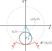
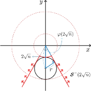
Figure 10: The geometric definitions of the superset $\bm{\mathcal{S}}^{+}(2\sqrt{n})$ (Left) and the subset $\bm{\mathcal{S}}^{-}(2\sqrt{n})$ (Right) of the set $\bm{\mathcal{S}}(2\sqrt{n})$ used in the proof of (v) in Lemma 5.

E. Proof of (v)

By (i) in Lemma 5, $\hat{P}=\text{P}\{\Delta\bm{V}\in\bm{\mathcal{S}}(2\sqrt{n})\}$. To derive a lower and upper bound on $\hat{P}$, we define a subset $\bm{\mathcal{S}}^{-}(2\sqrt{n})$ and a superset $\bm{\mathcal{S}}^{+}(2\sqrt{n})$ of the set $\bm{\mathcal{S}}(2\sqrt{n})$ as depicted in Fig. 10. Then, we have

$$\text{P}\{\Delta\bm{V}\in\bm{\mathcal{S}}^{-}(2\sqrt{n})\}\leq\hat{P}\leq\text{P}\{\Delta\bm{V}\in\bm{\mathcal{S}}^{+}(2\sqrt{n})\}.$$ (81)

By (iii) in Lemma 14, the probabilities $\text{P}\{\Delta\bm{V}\in\bm{\mathcal{S}}^{\pm}(2\sqrt{n})\}$ are obtained by (double sings in same order)

$$\text{P}\{\Delta\bm{V}\in\bm{\mathcal{S}}^{\pm}(2\sqrt{n})\}$$

$$\quad=1-\text{P}\{\Delta\bm{V}\notin\bm{\mathcal{S}}^{\pm}(2\sqrt{n})\}$$

$$\quad=1-\text{P}\{|\Delta\bm{V}|\geq 2\sqrt{n}\pm r\}\cdot\frac{\varphi(2\sqrt{n})}{2\pi},$$ (82)

where $\varphi(2\sqrt{n})$ is the central angle associated with $\bm{\mathcal{S}}^{\pm}(2\sqrt{n})$ (See Fig. 10). From the geometry in Fig. 10, the angle $\varphi(2\sqrt{n})$ is given by

$$\varphi(2\sqrt{n})=2\sin^{-1}\left(\frac{r}{2\sqrt{n}}\right).$$ (83)

We now consider the probabilities $\text{P}\{|\Delta\bm{V}|\geq 2\sqrt{n}\pm r\}$ in (E. Proof of (v)). For notational simplicity, we denote $\Delta\bm{V}=(\Delta V_{x},\Delta V_{y})$. Then, by (ii) in Lemma 14,

$$\Delta V_{x} \stackrel{{\scriptstyle\text{d}}}{{=}}Z_{i}(k)\cos\theta_{i}(k)-Z_{j}(k)\cos\theta_{j}(k),$$

$$\Delta V_{y} \stackrel{{\scriptstyle\text{d}}}{{=}}Z_{i}(k)\sin\theta_{i}(k)-Z_{j}(k)\sin\theta_{j}(k).$$

Note that for any $\bm{v}=(v_{x},v_{y})\in\mathbb{R}^{2}$ and $\eta\geq 0$, $|v_{x}|\geq\eta$ implies $|\bm{v}|\geq\eta$, and $|\bm{v}|\geq\eta$ implies $|v_{x}|\geq\eta/\sqrt{2}$ or $|v_{y}|\geq\eta/\sqrt{2}$. Hence, $\text{P}\{|\bm{v}|>\eta\}$ is bounded by

$$\text{P}\{|v_{x}|\geq\eta\} \leq\text{P}\{|\bm{v}|\geq\eta\}$$ (84a)

$$\leq\text{P}\{|v_{x}|\geq\eta/\sqrt{2}\text{ or }|v_{y}|\geq\eta/\sqrt{2}\}.$$ (84b)

Since $\theta_{i}(k)$ and $\theta_{j}(k)$ are independent and uniformly distributed over $(0,2\pi]$, $\Delta V_{x}$ is symmetric, i.e., $\Delta V_{x}\stackrel{{\scriptstyle\text{d}}}{{=}}-\Delta V_{x}$. Thus, applying (84a) with $\bm{v}=\Delta\bm{V}$ and $\eta=2\sqrt{n}+r$ yields

$$\text{P}\{|\Delta\bm{V}|\geq 2\sqrt{n}+r\} \geq\text{P}\{|\Delta V_{x}|\geq 2\sqrt{n}+r\}$$

$$=2\text{P}\{\Delta V_{x}\geq 2\sqrt{n}+r\}.$$

Since $z_{\text{th}}$ in Lemma 16 is a constant independent of $n$, there exists a constant $n_{\text{th},l}\in\mathbb{N}$ such that $2\sqrt{n}+r\geq 2z_{\text{th}}$ for all $n\geq n_{\text{th},l}$. Hence, by Lemma 16, we have for all $n\geq n_{\text{th},l}$

$$\text{P}\{|\Delta\bm{V}|\geq 2\sqrt{n}+r\} \geq 2c_{l}\left(\frac{1}{2\sqrt{n}+r}\right)^{\alpha}.$$ (85)

Since $\cos\theta\stackrel{{\scriptstyle\text{d}}}{{=}}\sin\theta$ for $\theta\sim\text{Uniform}[0,2\pi]$, $|\Delta V_{x}|\stackrel{{\scriptstyle\text{d}}}{{=}}|\Delta V_{y}|$. Thus, applying (84b) with $\bm{v}=\Delta\bm{V}$ and $\eta=2\sqrt{n}-r$ yields

$$\text{P}\{|\Delta\bm{V}|\geq 2\sqrt{n}-r\}$$

$$\leq\text{P}\{|\Delta V_{x}|\geq(2\sqrt{n}-r)/\sqrt{2}\text{ or }|\Delta V_{y}|\geq(2\sqrt{n}-r)/\sqrt{2}\}$$

$$\leq 2\text{P}\{|\Delta V_{x}|\geq(2\sqrt{n}-r)/\sqrt{2}\}$$

$$=4\text{P}\{\Delta V_{x}\geq(2\sqrt{n}-r)/\sqrt{2}\}.$$

By the same reason as above, there exists a constant $n_{\text{th},u}\in\mathbb{N}$ such that $(2\sqrt{n}-r)/\sqrt{2}\geq 2z_{\text{th}}$ for all $n\geq n_{\text{th},u}$. Hence, by Lemma 16, we have for all $n\geq n_{\text{th},u}$

$$\text{P}\{|\Delta\bm{V}|\geq 2\sqrt{n}-r\} \leq 2^{\alpha/2+2}c_{u}\left(\frac{1}{2\sqrt{n}-r}\right)^{\alpha}.$$ (86)

Combining (81), (E. Proof of (v)), (83), (85), and (86) yields

$$\hat{P} \leq 1-\frac{2c_{l}}{\pi}\left(\frac{1}{2\sqrt{n}+r}\right)^{\alpha}\sin^{-1}\left(\frac{r}{2\sqrt{n}}\right),$$

$$\hat{P} \geq 1-\frac{2^{\alpha/2+2}c_{u}}{\pi}\left(\frac{1}{2\sqrt{n}-r}\right)^{\alpha}\sin^{-1}\left(\frac{r}{2\sqrt{n}}\right),$$

for all $n\geq n_{\text{th}}\triangleq\max(n_{\text{th},l},n_{\text{th},u})$.

Proof of Lemma 8

To complete the proof of Lemma 8, it remains to show that (i) $(1-\hat{P})^{-1}=\Theta(n^{(1+\alpha)/2-\beta})$ and (ii) $\bar{D}_{\hat{\pi}}=O(n)$. Without loss of generality, we assume $r=n^{\beta}$ $(0\leq\beta\leq 1/4)$.

A. Proof of (i)

To prove (i), we need the following: for any $x\in[0,1]$,

$$x\leq\sin^{-1}\left(x\right)\leq\frac{\pi}{2}x.$$ (87)

The proof of (87) is given at the end of this section. From (19a) in Lemma 5 with $r=n^{\beta}$, we have for all $n\geq n_{\text{th}}$ the following:

$$1-\hat{P} \geq\frac{2c_{l}}{\pi}\left(\frac{1}{2\sqrt{n}+n^{\beta}}\right)^{\alpha}\sin^{-1}\left(\frac{n^{\beta-1/2}}{2}\right).$$

Since $\frac{n^{\beta-1/2}}{2}\in[0,1]$ for any $\beta\in[0,1/4]$ and $n\in\mathbb{N}$, we further have from the lower inequality in (87) that

$$1-\hat{P} \geq\frac{c_{l}}{\pi}\left(\frac{1}{2\sqrt{n}+n^{\beta}}\right)^{\alpha}n^{\beta-1/2}.$$

Hence, we have

$$\limsup_{n\to\infty}\frac{(1-\hat{P})^{-1}}{n^{(1+\alpha)/2-\beta}} \leq\frac{2^{\alpha}\pi}{c_{l}}<\infty,$$

which gives

$$(1-\hat{P})^{-1}=O(n^{(1+\alpha)/2-\beta}).$$ (88)

Using a similar approach as above, from (19b) in Lemma 5 and the upper inequality in (87), we have for all $n\geq n_{\text{th}}$ the following:

$$1-\hat{P} \leq 2^{\alpha/2}c_{u}\left(\frac{1}{2\sqrt{n}-n^{\beta}}\right)^{\alpha}n^{\beta-1/2}.$$

Hence, we have

$$\limsup_{n\to\infty}\frac{n^{(1+\alpha)/2-\beta}}{(1-\hat{P})^{-1}} \leq 2^{-\alpha/2}c_{u}<\infty,$$

which gives

$$(1-\hat{P})^{-1}=\Omega(n^{(1+\alpha)/2-\beta}).$$ (89)

Combining (88) and (89) proves (i).

Proof of (87): For $|x|\leq 1$, the function $\sin^{-1}\left(x\right)$ can be calculated using the following infinite series:

$$\sin^{-1}\left(x\right)=\sum_{l=0}^{\infty}d_{l}\,x^{2l+1},$$

where $d_{l}\triangleq\frac{(2l)!}{4^{l}(l!)^{2}(2l+1)}\,(>0)$. Hence, for any $x\in[0,1]$, we have a lower bound on $\sin^{-1}\left(x\right)$ as

$$\sin^{-1}\left(x\right)\geq d_{0}\,x=x.$$ (90)

Since $x^{2l+1}\leq x$ for all $l=0,1,\ldots$ and $x\in[0,1]$, we have

$$\sin^{-1}\left(x\right)\leq x\sum_{l=0}^{\infty}d_{l}.$$

Note that $\sum_{l=0}^{\infty}d_{l}=\sin^{-1}\left(1\right)=\frac{\pi}{2}$. Hence, for any $x\in[0,1]$, we have an upper bound on $\sin^{-1}\left(x\right)$ as

$$\sin^{-1}\left(x\right)\leq\frac{\pi}{2}x.$$ (91)

Combining (90) and (91) proves (87).

B. Proof of (ii)

Without loss of generality, we assume $\text{P}\{Z_{\alpha}>z_{\text{th}}\}=1$. (In this proof, subscript $\alpha$ is added to all random variables to specify the underlying parameter $\alpha$ of the Lévy flight model.) Then, from (6), we have $\text{P}\{Z_{\alpha}>z\}=(\frac{z_{\text{th}}}{z})^{\alpha}$ for all $z\geq z_{\text{th}}$, which gives for any $0<\alpha_{1}\leq\alpha_{2}\leq 2$ and $z\geq z_{\text{th}}$ the following:

$$\text{P}\{Z_{\alpha_{1}}>z\}=\Big{(}\frac{z_{\text{th}}}{z}\Big{)}^{\alpha_{1}}\geq\Big{(}\frac{z_{\text{th}}}{z}\Big{)}^{\alpha_{2}}=\text{P}\{Z_{\alpha_{2}}>z\}.$$ (92)

The inequality in (92) shows that for any $t_{2}>t_{1}\geq 0$ having a sufficiently small difference $\epsilon\triangleq t_{2}-t_{1}>0$, we get

$$\text{P}\{L_{\alpha_{1}}\!(t_{2})>r|L_{\alpha_{1}}\!(t_{1})>r\}\leq\text{P}\{L_{\alpha_{2}}\!(t_{2})>r|L_{\alpha_{2}}\!(t_{1})>r\},$$

which results in

$$\text{P}\{T_{\alpha_{1}}>t_{2}\,|\,T_{\alpha_{1}}>t_{1}\}\leq\text{P}\{T_{\alpha_{2}}>t_{2}\,|\,T_{\alpha_{2}}>t_{1}\}.$$ (93)

Note that since $\text{P}\{T_{\alpha_{1}}>t\}=\text{P}\{T_{\alpha_{1}}>t,T_{\alpha_{1}}>t-\epsilon\}$ for $t\geq\epsilon$, we can express $\text{P}\{T_{\alpha_{1}}>t\}$ in a nested form as

$$\text{P}\{T_{\alpha_{1}}>t\} =\text{P}\{T_{\alpha_{1}}>t\,|\,T_{\alpha_{1}}>t-\epsilon\}\text{P}\{T_{\alpha_{1}}>t-\epsilon\}.$$

Using the nested form continuously, we have

$$\text{P}\{T_{\alpha_{1}}>t\} =\text{P}\{T_{\alpha_{1}}>t\,|\,T_{\alpha_{1}}>t-\epsilon\}$$

$$\qquad\times\text{P}\{T_{\alpha_{1}}>t-\epsilon\,|\,T_{\alpha_{1}}>t-2\epsilon\}$$

$$\qquad\times\ldots$$

$$\qquad\times\text{P}\{T_{\alpha_{1}}>t-\lfloor t/\epsilon\rfloor\epsilon\,|\,T_{\alpha_{1}}>0\}$$

$$\qquad\times\text{P}\{T_{\alpha_{1}}>0\}.$$ (94)

Hence, by applying (93) to (B. Proof of (ii)), we have

$$\text{P}\{T_{\alpha_{1}}>t\} \leq\text{P}\{T_{\alpha_{2}}>t\,|\,T_{\alpha_{2}}>t-\epsilon\}$$

$$\qquad\times\text{P}\{T_{\alpha_{2}}>t-\epsilon\,|\,T_{\alpha_{2}}>t-2\epsilon\}$$

$$\qquad\times\ldots$$

$$\qquad\times\text{P}\{T_{\alpha_{2}}>t-\lfloor t/\epsilon\rfloor\epsilon\,|\,T_{\alpha_{2}}>0\}$$

$$\qquad\times\text{P}\{T_{\alpha_{1}}>0\}.$$ (95)

Note that $\text{P}\{T_{\alpha_{1}}>0\}=\text{P}\{L_{\alpha_{1}}(0)>r\}$. In addition, since $\bm{X}_{i}(0)\sim\text{Uniform}(\bm{\mathcal{D}})$ for all $i=1,\ldots,n$ regardless of $\alpha$, we have $\text{P}\{T_{\alpha_{1}}>0\}=\text{P}\{T_{\alpha_{2}}>0\}$. Thus, the right-hand side of (B. Proof of (ii)) boils down to $\text{P}\{T_{\alpha_{2}}>t\}$, and consequently

$$\text{P}\{T_{\alpha_{1}}>t\} \leq\text{P}\{T_{\alpha_{2}}>t\}\quad\text{for all }t\geq 0.$$ (96)

Due to the property in (96), the average delay under the Lévy flight model with a parameter $\alpha\in(0,2)$ is dominated by the one under Brownian motion $(\alpha=2)$, which is shown to be $O(n)$ [8], i.e.,

$$\bar{D}_{\hat{\pi}}=O(n)\quad\text{for all }\alpha\in(0,2].$$

Appendix C Proofs of Lemmas for the i.i.d. Mobility Model

Here, we give detailed proofs of Lemmas 10 and 13, which are used for analyzing the optimal delay under the i.i.d. mobility model. To prove Lemma 10, we need the following Lemmas 17, 18, and 19.

Lemma 17.

For $i\neq j$ and $t\geq 0$, let

$$\Delta\bm{X}_{(i,j)}(t)\triangleq\bm{X}_{i}(t)-\bm{X}_{j}(t),$$

where $\bm{X}_{\cdot}(t)$ denotes the location of a node $\cdot$ at time $t$. Then, under the i.i.d. mobility model, $\Delta\bm{X}_{(i,j)}(t)$ has the following properties:
(i) $\Delta\bm{X}_{(i,j)}(k)\,(k\in\mathbb{N})$ is independent of $\bm{X}_{u}(t)$ for all $u=1,\ldots,n$ and $t\in[0,k-1]$.
(ii) $\Delta\bm{X}_{(i,j)}(t)$ is identically distributed across pair index $(i,j)$ and time $t\,(\geq 0)$. Hence, we use $\Delta\bm{X}$ to denote a generic random variable for $\Delta\bm{X}_{(i,j)}(t)$.
(iii) The angle $\angle\Delta\bm{X}$ is a uniform random variable on the interval $(0,2\pi]$ and is independent of the length $|\Delta\bm{X}|$.

Proof: (i) For any $u=1,\ldots,n$, $\bm{X}_{u}(t)\,(0\leq t\leq k-1)$ under the i.i.d. mobility model is completely determined by $\bm{G}_{u}(k-1)\triangleq\{\bm{X}_{u}(0),\ldots,\bm{X}_{u}(k-1)\}$ (by the relation (1)). Since $\bm{X}_{i}(k)$ is independent of $\bm{G}_{u}(k-1)$, it is independent of $\bm{X}_{u}(t)$. By the same reason, $\bm{X}_{j}(k)$ is independent of $\bm{X}_{u}(t)$. Therefore, the difference $\bm{X}_{i}(k)-\bm{X}_{j}(k)$ is independent of $\bm{X}_{u}(t)$.
(ii) For any $i\neq j$ and $t\geq 0$, $\bm{X}_{i}(t)$ and $\bm{X}_{j}(t)$ are independent and identically distributed. Therefore, the difference $\bm{X}_{i}(t)-\bm{X}_{j}(t)$ is identically distributed across pair index $(i,j)$ and time $t$. However, it is not necessarily independent neither across $(i,j)$ nor across $t$.
(iii) To prove (iii), it suffices to show that for any $x\geq 0$,

$$\text{P}\big{\{}\angle\Delta\bm{X}\leq\theta\,\big{|}\,|\Delta\bm{X}|=x\big{\}}=\frac{\theta}{2\pi},$$ (97)

where $0<\theta\leq 2\pi$. By noting that $\angle\bm{X}_{i}(t)\sim\text{Uniform}[0,2\pi]$ for any $i=1,\ldots,n$ and $t\geq 0$ and using a similar approach as in the proof of (iii) in Lemma 14, we can prove (iii) in Lemma 17. Due to similarities, we omit the details. $\blacksquare$

Lemma 18.

Suppose $k\in\mathbb{N}$ and $l\in(r,2\sqrt{n}]$. Then, for any sets $\mathcal{L}(\cdot)\subset[0,2\sqrt{n}]$ satisfying

$$\text{P}\{L(k-1)=l,L(t)\in\mathcal{L}(t),0\leq t\leq k-1\}>0,$$

we have under the i.i.d. mobility model the following:

$$\text{P}\{I(k)=0\,|\,L(k-1)=l,L(t)\in\mathcal{L}(t),0\leq t\leq k-1\}$$

$$\quad=\text{P}\{\Delta\bm{X}\in\bm{\mathcal{S}}^{\star}(l)\}.$$ (98)

The definitions of $\Delta\bm{X}$ and $\bm{\mathcal{S}}^{\star}(l)$ can be found in Lemma 10.

Remark 2.

Before proving the lemma, we give a remark. As Lemma 15 for the Lévy flight model, Lemma 18 implies that the future states of a meeting process under the i.i.d. mobility model depend only on the state at the beginning of the current slot, not on the sequence of events that preceded it. In addition, the conditional probability distribution of the future state described above is time homogeneous (i.e., the probability in (18) does not depend on the slot index $k$). This restricted time homogeneous memoryless property enables us to derive a bound on the first meeting time distribution as a geometric form (See Lemma 11).

Proof: Using a similar approach as in the proof of Lemma 15, we can prove Lemma 18. The difference is that the key idea of this proof is to use the following equality: for any $k\in\mathbb{N}$, $l\in(r,2\sqrt{n}]$, $\theta\in(0,2\pi]$, and $\mathcal{F}(k-1)$, we have

$$\text{P}\{I(k)=0\,|\,\Delta\bm{X}(k-1)=l\bm{e}^{j\theta},\mathcal{F}(k-1)\}$$

$$\quad=\text{P}\{\Delta\bm{X}\in\bm{\mathcal{S}}^{\star}(l)\},$$ (99)

where the definition of $\mathcal{F}(k-1)$ can be found in (57). Then, similarly to the proof of Lemma 15, using the key equality in (C) we can prove Lemma 18. Due to similarities, we omit the details.

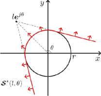
Figure 11: An example of $\bm{\mathcal{S}}^{\star}(l,\theta)$: when $\theta=\frac{\pi}{2}$, $\bm{\mathcal{S}}^{\star}(l,\theta)$ is identical to $\bm{\mathcal{S}}^{\star}(l)$.

In the following, we show (C). We first consider the event $\{I(k)=0\}$. Since (61) also holds for the i.i.d. mobility model, by the same reason in the proof of Lemma 15, the event $\{I(k)=0\}$ occurs if and only if the following event occurs:

$$\Big{\{}\overline{\big{(}\Delta\bm{X}(k-1),\Delta\bm{X}(k)\big{)}}\cap\bm{\mathcal{D}}_{r}(\bm{0})=\varnothing\Big{\}}.$$ (100)

We next consider the event $\{I(k)=0\}$ conditioned by $\Delta\bm{X}(k-1)=l\bm{e}^{j\theta}$ and $\mathcal{F}(k-1)$. Under these conditions, (100) is reduced to the following:

$$\Big{\{}\overline{\big{(}\Delta\bm{X}(k-1),\Delta\bm{X}(k)\big{)}}\cap\bm{\mathcal{D}}_{r}(\bm{0})=\varnothing\Big{\}}$$

$$\quad=\Big{\{}\overline{\big{(}l\bm{e}^{j\theta},\Delta\bm{X}(k)\big{)}}\cap\bm{\mathcal{D}}_{r}(\bm{0})=\varnothing\Big{\}}$$

$$\quad=\Big{\{}\Delta\bm{X}(k)\in\bm{\mathcal{S}}^{\star}(l,\theta)\Big{\}},$$

where

$$\bm{\mathcal{S}}^{\star}(l,\theta) \triangleq\big{\{}\bm{x}\in\mathbb{R}^{2}\,\big{|}\,\overline{\big{(}l\bm{e}^{j\theta},\bm{x}\big{)}}\cap\bm{\mathcal{D}}_{r}(\bm{0})=\varnothing\big{\}}.$$

An example of $\bm{\mathcal{S}}^{\star}(l,\theta)$ is shown in Fig. 11. Hence, the probability on the left-hand side of (C) becomes

$$\text{P}\{I(k)=0\,|\,\Delta\bm{X}(k\!-\!1)=l\bm{e}^{j\theta},\mathcal{F}(k\!-\!1)\}$$

$$=\text{P}\{\Delta\bm{X}(k)\!\in\!\bm{\mathcal{S}}^{\star}(l,\theta)|\Delta\bm{X}(k\!-\!1)=l\bm{e}^{j\theta},\mathcal{F}(k\!-\!1)\}.$$ (101)

By (i) in Lemma 17, $\Delta\bm{X}(k)$ is independent of $\Delta\bm{X}(k-1)$ and $\mathcal{F}(k-1)$, and thus we have

$$\text{P}\{\Delta\bm{X}(k)\in\bm{\mathcal{S}}^{\star}(l,\theta)\,|\,\Delta\bm{X}(k-1)=l\bm{e}^{j\theta},\mathcal{F}(k-1)\}$$

$$\quad=\text{P}\{\Delta\bm{X}(k)\in\bm{\mathcal{S}}^{\star}(l,\theta)\}.$$ (102)

In addition, by (ii) in Lemma 17,

$$\text{P}\{\Delta\bm{X}(k)\in\bm{\mathcal{S}}^{\star}(l,\theta)\} =\text{P}\{\Delta\bm{X}\in\bm{\mathcal{S}}^{\star}(l,\theta)\}.$$ (103)

Finally, by (iii) in Lemma 17, the probability in (103) is invariant for any $\theta\in(0,2\pi]$. When $\theta=\frac{\pi}{2}$, we have $\bm{\mathcal{S}}^{\star}(l,\frac{\pi}{2})=\bm{\mathcal{S}}^{\star}(l)$. Hence, the following holds for any $\theta\in(0,2\pi]$:

$$\text{P}\{\Delta\bm{X}\in\bm{\mathcal{S}}^{\star}(l,\theta)\} =\text{P}\{\Delta\bm{X}\in\bm{\mathcal{S}}^{\star}(l)\}.$$ (104)

Combining (C), (C), (103), and (104) gives (C). This completes the proof. $\blacksquare$

Lemma 19.

Let $f_{|\Delta\bm{X}|}(\cdot)$ denote the probability density function of the random variable $|\Delta\bm{X}|$ under the i.i.d. mobility model. Then, it is bounded by

$$f_{|\Delta\bm{X}|}(x)\leq\frac{2x}{n},\quad\text{ for all }x\in[0,2\sqrt{n}].$$

Proof: We will prove this lemma by showing the following:

$$\limsup_{\epsilon\downarrow 0}\frac{\text{P}\{x-\frac{\epsilon}{2}\leq|\Delta\bm{X}|\leq x+\frac{\epsilon}{2}\}}{\epsilon}\leq\frac{2x}{n}.$$ (105)

From (ii) in Lemma 17, we have $|\Delta\bm{X}|\stackrel{{\scriptstyle\text{d}}}{{=}}|\Delta\bm{X}_{(i,j)}(0)|$. Hence, by conditioning on the values of $\bm{X}_{i}(0)$, the probability in (105) can be rewritten as

$$\text{P}\Big{\{}x-\frac{\epsilon}{2}\leq|\Delta\bm{X}|\leq x+\frac{\epsilon}{2}\Big{\}}$$

$$=\int_{\bm{\mathcal{D}}}\text{P}\Big{\{}x\!-\!\frac{\epsilon}{2}\!\leq\!|\Delta\bm{X}_{(i,j)}(0)|\!\leq\!x\!+\!\frac{\epsilon}{2}\Big{|}\bm{X}_{i}(0)\!=\!\bm{u}\Big{\}}\text{d}F_{\!\bm{X}_{i}(0)}(\bm{u})$$

$$=\int_{\bm{\mathcal{D}}}\text{P}\{\bm{X}_{j}(0)\in\bm{\mathcal{R}}_{(x,\epsilon)}(\bm{u})\,|\,\bm{X}_{i}(0)=\bm{u}\}\,\text{d}F_{\bm{X}_{i}(0)}(\bm{u}),$$

where $\bm{\mathcal{R}}_{(x,\epsilon)}(\bm{u})\triangleq\{\bm{v}\in\mathbb{R}^{2}\,|\,x-\frac{\epsilon}{2}\leq|\bm{v}-\bm{u}|\leq x+\frac{\epsilon}{2}\}$. By independence between $\bm{X}_{i}(0)$ and $\bm{X}_{j}(0)$, we further have

$$\begin{split}&\text{P}\Big{\{}x-\frac{\epsilon}{2}\leq|\Delta\bm{X}|\leq x+\frac{\epsilon}{2}\Big{\}}\\ &\quad=\int_{\bm{\mathcal{D}}}\text{P}\{\bm{X}_{j}(0)\in\bm{\mathcal{R}}_{(x,\epsilon)}(\bm{u})\}\,\text{d}F_{\bm{X}_{i}(0)}(\bm{u}).\end{split}$$ (106)

Note that, since $\bm{X}_{j}(0)\in\bm{\mathcal{D}}$ with probability 1 and $\bm{X}_{j}(0)\sim\text{Uniform}(\bm{\mathcal{D}})$, the probability $\text{P}\{\bm{X}_{j}(0)\in\bm{\mathcal{R}}_{(x,\epsilon)}(\bm{u})\}$ in the integral in (106) is given by

$$\text{P}\{\bm{X}_{j}(0)\in\bm{\mathcal{R}}_{(x,\epsilon)}(\bm{u})\} =\frac{\text{Area}(\bm{\mathcal{D}}\cap\bm{\mathcal{R}}_{(x,\epsilon)}(\bm{u}))}{\text{Area}(\bm{\mathcal{D}})}$$

$$\leq\frac{\text{Area}(\bm{\mathcal{R}}_{(x,\epsilon)}(\bm{u}))}{\pi n}.$$ (107)

In addition, for any $\bm{u}\in\bm{\mathcal{D}}$ and sufficiently small $\epsilon\,(>0)$, the area $\text{Area}(\bm{\mathcal{R}}_{(x,\epsilon)}(\bm{u}))$ is calculated as

$$\text{Area}(\bm{\mathcal{R}}_{(x,\epsilon)}(\bm{u})) =\begin{cases}\pi(x+\frac{\epsilon}{2})^{2}-\pi(x-\frac{\epsilon}{2})^{2},&\text{ if }x>0,\\ \pi(x+\frac{\epsilon}{2})^{2},&\text{ if }x=0,\end{cases}$$

$$=\begin{cases}2\pi x\epsilon,&\text{ if }x>0,\\ \frac{\pi\epsilon^{2}}{4},&\text{ if }x=0.\end{cases}$$ (108)

By applying the combined result of (C) and (C) to (106), we have

$$\text{P}\Big{\{}x-\frac{\epsilon}{2}\leq|\Delta\bm{X}|\leq x+\frac{\epsilon}{2}\Big{\}}\leq\begin{cases}\frac{2x\epsilon}{n},&\text{ if }x>0,\\ \frac{\epsilon^{2}}{4n},&\text{ if }x=0,\end{cases}$$

which gives

$$\limsup_{\epsilon\downarrow 0}\frac{\text{P}\{x-\frac{\epsilon}{2}\leq|\Delta\bm{X}|\leq x+\frac{\epsilon}{2}\}}{\epsilon} \leq\begin{cases}\frac{2x}{n},&\text{ if }x>0,\\ 0,&\text{ if }x=0,\end{cases}$$

$$=\frac{2x}{n}.$$

This proves the lemma. $\blacksquare$

Proof of Lemma 10

A. Proof of (i)

Similarly to the proof of (i) in Lemma 5, we can prove (i) in Lemma 10 by applying Lemma 18 with $k=1$, $l=l_{0}$, and $\mathcal{L}(0)=(r,2\sqrt{n}]$. Due to similarities, we omit the details.

B. Proof of (ii)

Suppose $r<l_{0}\leq l_{1}\leq 2\sqrt{n}$. Then, it is obvious from the definition of $\bm{\mathcal{S}}^{\star}(\cdot)$ in (35) that $\bm{\mathcal{S}}^{\star}(l_{0})\subseteq\bm{\mathcal{S}}^{\star}(l_{1})$ (See Fig. 5). Hence, we have

$$\text{P}\{\Delta\bm{X}\in\bm{\mathcal{S}}^{\star}(l_{0})\} \leq\text{P}\big{\{}\Delta\bm{X}\in\bm{\mathcal{S}}^{\star}(l_{1})\big{\}},$$

which is equivalent to $H(1,l_{0})\leq H(1,l_{1})$ by (i) in Lemma 10.

C. Proof of (iii)

By (ii) in Lemma 10, we have $H(1,l_{0})\leq H(1,2\sqrt{n})\,(=\hat{P})$ for any $l_{0}\in(r,2\sqrt{n}]$.

D. Proof of (iv)

By following the approach in the proof of (iv) in Lemma 5, we can prove (iv) in Lemma 10 based on Lemma 18 and (i) and (iii) in Lemma 10. Due to similarities, we omit the details.

Figure 12: The geometric definition of $\phi(x)$: it is the central angle of the arc $\{\bm{x}\in\bm{\mathcal{S}}^{\star}(2\sqrt{n})||\bm{x}|=x\}$ depicted in red.

E. Proof of (v)

By (i) in Lemma 10 and (iii) in Lemma 17, we have

$$\hat{P} =\text{P}\{\Delta\bm{X}\in\bm{\mathcal{S}}^{\star}(2\sqrt{n})\}$$

$$=\int_{r^{+}}^{2\sqrt{n}}\frac{\phi(x)}{2\pi}f_{|\Delta\bm{X}|}(x)\,\text{d}x,$$ (109)

where $\phi(x)$ is the central angle of the arc $\{\bm{x}\!\in\!\bm{\mathcal{S}}^{\star}(2\sqrt{n})||\bm{x}|=x\}$ (See Fig. 12), and $f_{|\Delta\bm{X}|}(\cdot)$ is defined in Lemma 19. From the geometry in Fig. 12, the angle $\phi(x)$ is given by

$$\phi(x) =2\cos^{-1}\Big{(}\frac{r}{2\sqrt{n}}\Big{)}+2\cos^{-1}\Big{(}\frac{r}{x}\Big{)}$$

$$=2\pi-2\sin^{-1}\Big{(}\frac{r}{2\sqrt{n}}\Big{)}-2\sin^{-1}\Big{(}\frac{r}{x}\Big{)},$$ (110)

where the second equality comes from the identity $\cos^{-1}(\theta)=\frac{\pi}{2}-\sin^{-1}(\theta)$ $(-\frac{\pi}{2}\leq\theta\leq\frac{\pi}{2})$. By substituting (E. Proof of (v)) into (E. Proof of (v)), we have

$$\begin{split}\hat{P}&=\Big{(}1-\frac{1}{\pi}\sin^{-1}\Big{(}\frac{r}{2\sqrt{n}}\Big{)}\Big{)}\cdot\text{P}\{|\Delta\bm{X}|>r\}\\ &\qquad-\frac{1}{\pi}\int_{r^{+}}^{2\sqrt{n}}\sin^{-1}\Big{(}\frac{r}{x}\Big{)}f_{|\Delta\bm{X}|}(x)\,\text{d}x.\end{split}$$ (111)

Based on (111), we derive an upper bound on $\hat{P}$ as follows:

$$\hat{P} \leq\Big{(}1-\frac{1}{\pi}\sin^{-1}\Big{(}\frac{r}{2\sqrt{n}}\Big{)}\Big{)}\cdot\text{P}\{|\Delta\bm{X}|>r\}$$

$$\leq 1-\frac{1}{\pi}\sin^{-1}\Big{(}\frac{r}{2\sqrt{n}}\Big{)}.$$

This proves the upper bound in (36a).

Using (111) again, we derive a lower bound on $\hat{P}$ as follows: since $|\Delta\bm{X}|\stackrel{{\scriptstyle\text{d}}}{{=}}|\Delta\bm{X}(0)|$ by (ii) in Lemma 17 and $|\Delta\bm{X}(0)|=L(0)$ by definition, we have $\text{P}\{|\Delta\bm{X}|>r\}=\text{P}\{L(0)>r\}$. Hence, by Lemma 3, the probability $\text{P}\{|\Delta\bm{X}|>r\}$ in (111) is bounded by

$$\text{P}\{|\Delta\bm{X}|>r\}=P_{o}\geq 1-\frac{r}{n^{2}}.$$ (112)

By Lemma 19, the integral in (111) is bounded by

$$\int_{r^{+}}^{2\sqrt{n}}\sin^{-1}\Big{(}\frac{r}{x}\Big{)}f_{|\Delta\bm{X}|}(x)\,\text{d}x \leq\frac{2}{n}\int_{r^{+}}^{2\sqrt{n}}\sin^{-1}\Big{(}\frac{r}{x}\Big{)}x\,\text{d}x.$$ (113)

Let $y\triangleq r/x$. By the change of variables, the integral on the right-hand side of (113) is solved as

$$\frac{2}{n}\int_{r^{+}}^{2\sqrt{n}}\sin^{-1}\Big{(}\frac{r}{x}\Big{)}x\,\text{d}x$$

$$\quad=-\frac{\pi r^{2}}{2n}+\frac{2r}{\sqrt{n}}\sqrt{1-\frac{r^{2}}{4n}}+4\sin^{-1}\Big{(}\frac{r}{2\sqrt{n}}\Big{)}.$$ (114)

By applying (112), (113), and (E. Proof of (v)) to (111), we have

$$\hat{P} \geq\Big{(}1-\frac{1}{\pi}\sin^{-1}\Big{(}\frac{r}{2\sqrt{n}}\Big{)}\Big{)}\cdot\Big{(}1-\frac{r^{2}}{n}\Big{)}$$

$$\qquad+\frac{r^{2}}{2n}-\frac{2r}{\pi\sqrt{n}}\sqrt{1-\frac{r^{2}}{4n}}-\frac{4}{\pi}\sin^{-1}\Big{(}\frac{r}{2\sqrt{n}}\Big{)}$$

$$\geq 1-\frac{r^{2}}{2n}-\frac{2r}{\pi\sqrt{n}}-\frac{5}{\pi}\sin^{-1}\Big{(}\frac{r}{2\sqrt{n}}\Big{)}.$$

This proves the lower bound in (36b).

Proof of Lemma 13

Order of $\bar{U}(1)$: To complete the proof of (43), it remains to show $(1-\hat{P})^{-1}=\Theta(n^{1/2-\beta})$. For this, we will show the followings:

$$\text{(i)}~{}(1-\hat{P})^{-1}=O(n^{1/2-\beta}),$$

$$\text{(ii)}~{}(1-\hat{P})^{-1}=\Omega(n^{1/2-\beta}).$$

Without loss of generality, we assume $r=n^{\beta}\,(0\leq\beta\leq 1/4)$ in the rest of this appendix. From (36a) in Lemma 10 with $r=n^{\beta}$, we have for all $n\in\mathbb{N}$ the following:

$$1-\hat{P}\geq\frac{1}{\pi}\sin^{-1}\Big{(}\frac{n^{\beta-1/2}}{2}\Big{)}.$$

Since $\frac{n^{\beta-1/2}}{2}\in[0,1]$ for any $\beta\in[0,1/4]$ and $n\in\mathbb{N}$, we further have from the lower inequality in (87) (i.e., $x\leq\sin^{-1}\left(x\right)$ for any $x\in[0,1]$) that

$$1-\hat{P}\geq\frac{n^{\beta-1/2}}{2\pi}.$$ (115)

Hence, we have

$$\limsup_{n\to\infty}\frac{(1-\hat{P})^{-1}}{n^{1/2-\beta}} \leq 2\pi<\infty,$$

which proves (i) $(1-\hat{P})^{-1}=O(n^{1/2-\beta})$.

Using a similar approach as above, from (36b) in Lemma 10 and the upper inequality in (87) (i.e., $\sin^{-1}\left(x\right)\leq\frac{\pi}{2}x$ for any $x\in[0,1]$), we have for all $n\in\mathbb{N}$ the following:

$$1-\hat{P} \leq\frac{n^{2\beta-1}}{2}+\frac{2n^{\beta-1/2}}{\pi}+\frac{5}{\pi}\sin^{-1}\Big{(}\frac{n^{\beta-1/2}}{2}\Big{)}$$

$$\leq\frac{n^{\beta-1/2}}{2}+\frac{2n^{\beta-1/2}}{\pi}+\frac{5n^{\beta-1/2}}{4}$$

$$=\Big{(}\frac{2}{\pi}+\frac{7}{4}\Big{)}n^{\beta-1/2}.$$ (116)

Hence, we have

$$\limsup_{n\to\infty}\frac{n^{1/2-\beta}}{(1-\hat{P})^{-1}} \leq\frac{2}{\pi}+\frac{7}{4}<\infty,$$

which proves (ii) $(1-\hat{P})^{-1}=\Omega(n^{1/2-\beta})$.

Order of $\bar{U}(\lceil\gamma r^{2}\rceil)$: To complete the proof of (44), it remains to show $(1-(\hat{P})^{\lceil\gamma r^{2}\rceil})^{-1}=\Theta(n^{\max(0,1/2-3\beta)})$. For this, we will show the followings:

$$\text{(iii)}~{}(1-(\hat{P})^{\lceil\gamma r^{2}\rceil})^{-1}=O(n^{\max(0,1/2-3\beta)}),$$

$$\text{(iv)}~{}(1-(\hat{P})^{\lceil\gamma r^{2}\rceil})^{-1}=\Omega(n^{\max(0,1/2-3\beta)}).$$

From (115), we have

$$1-(\hat{P})^{\lceil\gamma r^{2}\rceil} \geq 1-\Big{(}1-\frac{n^{\beta-1/2}}{2\pi}\Big{)}^{\lceil\gamma r^{2}\rceil}.$$ (117)

To simplify (117), we will use the following bound: for any $x\in[0,1]$ and $y>0$,

$$1-x^{\lceil y\rceil} =(1-x)(1+x+\ldots+x^{\lceil y\rceil-1})$$

$$\geq(1-x)\lceil y\rceil x^{\lceil y\rceil-1}$$

$$\geq(1-x)yx^{y}.$$ (118)

By applying (Proof of Lemma 13) with $x=1-\frac{n^{\beta-1/2}}{2\pi}\,(\in[0,1])$ and $y=\gamma r^{2}=\gamma n^{2\beta}\,(>0)$ to the right-hand side of (117), we have

$$1-(\hat{P})^{\lceil\gamma r^{2}\rceil} \geq\frac{\gamma n^{3\beta-1/2}}{2\pi}\Big{(}1-\frac{n^{\beta-1/2}}{2\pi}\Big{)}^{\gamma n^{2\beta}}.$$

Hence, we have

$$\limsup_{n\to\infty}\frac{\big{(}\!1-(\hat{P})^{\lceil\gamma r^{2}\rceil}\!\big{)}^{-1}}{n^{1/2-3\beta}} \leq\frac{2\pi}{\gamma}\limsup_{n\to\infty}\Big{(}\!1\!-\!\frac{n^{\beta-1/2}}{2\pi}\!\Big{)}^{-\gamma n^{2\beta}}.$$ (119)

To obtain the order of $(1-\frac{n^{\beta-1/2}}{2\pi})^{-\gamma n^{2\beta}}$, we take a logarithm function on it and then analyze the limiting behavior:

$$\lim_{n\to\infty}\log\Big{(}1\!-\!\frac{n^{\beta-1/2}}{2\pi}\Big{)}^{-\gamma n^{2\beta}}$$

$$\quad=\lim_{n\to\infty}\log\Big{(}1-\frac{n^{\beta-1/2}}{2\pi}\Big{)}^{n^{1/2-\beta}(-\gamma)n^{3\beta-1/2}}$$

$$\quad=-\gamma\lim_{n\to\infty}\bigg{(}n^{3\beta-1/2}\log\Big{(}1-\frac{n^{\beta-1/2}}{2\pi}\Big{)}^{n^{1/2-\beta}}\bigg{)}$$

$$\quad=-\gamma\lim_{n\to\infty}n^{3\beta-1/2}\cdot\lim_{n\to\infty}\log\Big{(}1-\frac{n^{\beta-1/2}}{2\pi}\Big{)}^{n^{1/2-\beta}}$$

$$\quad=\frac{\gamma}{2\pi}\lim_{n\to\infty}n^{3\beta-1/2}.$$ (120)

Hence, we have $\lim_{n\to\infty}\log(1-\frac{n^{\beta-1/2}}{2\pi})^{-\gamma n^{2\beta}}=0$ for $\beta\in[0,1/6)$. That is,

$$\lim_{n\to\infty}\Big{(}1-\frac{n^{\beta-1/2}}{2\pi}\Big{)}^{-\gamma n^{2\beta}}=1.$$ (121)

By combining (119) and (121), for $\beta\in[0,1/6)$ we obtain

$$\limsup_{n\to\infty}\frac{\big{(}1-(\hat{P})^{\lceil\gamma r^{2}\rceil}\big{)}^{-1}}{n^{1/2-3\beta}} \leq\frac{2\pi}{\gamma}<\infty,$$

which results in

$$\big{(}1-(\hat{P})^{\lceil\gamma r^{2}\rceil}\big{)}^{-1}\!=\!O(n^{1/2-3\beta}),\quad\text{for }\beta\in[0,1/6).$$ (122)

From (117), we have $1-(\hat{P})^{\lceil\gamma r^{2}\rceil}\geq 1-(1-\frac{n^{\beta-1/2}}{2\pi})^{\gamma n^{2\beta}}.$ Hence, we have

$$\begin{split}&\limsup_{n\to\infty}\frac{\big{(}1-(\hat{P})^{\lceil\gamma r^{2}\rceil}\big{)}^{-1}}{n^{0}}\\ &\quad\leq\frac{1}{\lim_{n\to\infty}1-\Big{(}1-\frac{n^{\beta-1/2}}{2\pi}\Big{)}^{\gamma n^{2\beta}}}.\end{split}$$ (123)

The limit $\lim_{n\to\infty}(1-\frac{n^{\beta-1/2}}{2\pi})^{\gamma n^{2\beta}}$ is obtained from (Proof of Lemma 13) as follows:

$$\lim_{n\to\infty}\log\Big{(}1\!-\!\frac{n^{\beta\!-\!1/2}}{2\pi}\Big{)}^{\gamma n^{2\beta}} =-\lim_{n\to\infty}\log\Big{(}1\!-\!\frac{n^{\beta\!-\!1/2}}{2\pi}\Big{)}^{-\gamma n^{2\beta}}$$

$$=\begin{cases}-\frac{\gamma}{2\pi},&\text{if }\beta=1/6,\\ -\infty,&\text{if }\beta\in(1/6,1/4].\end{cases}$$

That is,

$$\lim_{n\to\infty}\Big{(}1-\frac{n^{\beta-1/2}}{2\pi}\Big{)}^{\gamma n^{2\beta}} =\begin{cases}\exp(-\frac{\gamma}{2\pi}),&\text{if }\beta=1/6,\\ 0,&\text{if }\beta\in(1/6,1/4].\end{cases}$$ (124)

By substituting (124) into (123), for $\beta\in[1/6,1/4]$ we obtain

$$\limsup_{n\to\infty}\frac{\big{(}\!1\!-\!(\hat{P})^{\lceil\gamma r^{2}\rceil}\!\big{)}^{-1}}{n^{0}} \leq\begin{cases}\frac{1}{1-\exp(\!-\!\frac{\gamma}{2\pi})},&\text{if }\beta=1/6,\\ 1,&\text{if }\beta\in(1/6,1/4],\end{cases}$$

$$<\infty,$$

which results in

$$\big{(}1-(\hat{P})^{\lceil\gamma r^{2}\rceil}\big{)}^{-1}=O(n^{0}),\quad\text{ for }\beta\in[1/6,1/4].$$ (125)

Combining (122) and (125) proves (iii).

From (Proof of Lemma 13), we have

$$1-(\hat{P})^{\lceil\gamma r^{2}\rceil} \leq 1-\Big{(}1-\Big{(}\frac{2}{\pi}+\frac{7}{4}\Big{)}n^{\beta-1/2}\Big{)}^{\lceil\gamma r^{2}\rceil}.$$ (126)

To simplify (126), we will use the following bound: for any $x\in[0,1]$ and $y>0$,

$$1-x^{\lceil y\rceil} =(1-x)(1+x+\ldots+x^{\lceil y\rceil-1})$$

$$\leq(1-x)\lceil y\rceil.$$ (127)

By applying (Proof of Lemma 13) with $x=1-(\frac{2}{\pi}+\frac{7}{4})n^{\beta-1/2}\,(\in[0,1])$ and $y=\gamma r^{2}=\gamma n^{2\beta}\,(>0)$ to the right-hand side of (126), we have

$$1-(\hat{P})^{\lceil\gamma r^{2}\rceil} \leq\Big{(}\frac{2}{\pi}+\frac{7}{4}\Big{)}n^{\beta-1/2}\lceil\gamma n^{2\beta}\rceil.$$

Hence, we have

$$\limsup_{n\to\infty}\frac{n^{1/2-3\beta}}{\big{(}1-(\hat{P})^{\lceil\gamma r^{2}\rceil}\big{)}^{-1}} \leq\Big{(}\frac{2}{\pi}+\frac{7}{4}\Big{)}\lceil\gamma\rceil<\infty,$$

which results in

$$\big{(}1-(\hat{P})^{\lceil\gamma r^{2}\rceil}\big{)}^{-1}=\Omega(n^{1/2-3\beta}),\quad\text{for }\beta\in[0,1/4].$$ (128)

In addition, since $1-(\hat{P})^{\lceil\gamma r^{2}\rceil}\leq 1$, we have

$$\limsup_{n\to\infty}\frac{n^{0}}{\big{(}1-(\hat{P})^{\lceil\gamma r^{2}\rceil}\big{)}^{-1}} \leq 1<\infty,$$

which results in

$$\big{(}1-(\hat{P})^{\lceil\gamma r^{2}\rceil}\big{)}^{-1}=\Omega(n^{0}),\quad\text{ for }\beta\in[0,1/4].$$ (129)

Combining (128) and (129) proves (iv).

Order of $\text{P}\{B_{(n-2,P_{o}^{c})}\leq\lceil\gamma r^{2}\rceil-2\}$: By Chernoff’s inequality, the lower tail of the distribution function of the binomial random variable $B_{(n-2,P_{o}^{c})}$ for $x\leq(n-2)P_{o}^{c}$ is bounded by

$$\text{P}\{B_{(n-2,P_{o}^{c})}\leq x\} \leq\exp\Big{(}-\frac{((n-2)P_{o}^{c}-x)^{2}}{2(n-2)P_{o}^{c}}\Big{)}.$$ (130)

From Lemma 3, we have $P_{o}^{c}=1-P_{o}\geq\frac{r^{2}}{3n}$. Suppose $0<\gamma<\frac{1}{3}$ and $n\geq\frac{2}{1-3\gamma}$ (or, equivalently, $n-2\geq 3\gamma n$). Then, we have $(n-2)P_{o}^{c}\geq(n-2)\frac{r^{2}}{3n}\geq 3\gamma n\frac{r^{2}}{3n}=\gamma r^{2}$. Hence, we can apply $x=\gamma r^{2}$ to (130) under the conditions $0<\gamma<\frac{1}{3}$ and $n\geq\frac{2}{1-3\gamma}$, and we obtain

$$\text{P}\{B_{(n-2,P_{o}^{c})}\!\leq\!\gamma r^{2}\} \leq\exp\Big{(}\!-\!\frac{((n-2)P_{o}^{c}\!-\!\gamma r^{2})^{2}}{2(n-2)P_{o}^{c}}\Big{)}.$$ (131)

Since $P_{o}^{c}\geq\frac{r^{2}}{3n}$ and $n-2\geq 3\gamma n$, the term $(n-2)P_{o}^{c}-\gamma r^{2}$ in (131) is bounded below by

$$(n\!-\!2)P_{o}^{c}\!-\!\gamma r^{2} \geq(n\!-\!2)\frac{r^{2}}{3n}\!-\!\gamma r^{2}\!=\!\frac{n\!-\!2\!-\!3\gamma n}{3n}r^{2}\,(\geq 0),$$

from which we have

$$\big{(}(n-2)P_{o}^{c}-\gamma r^{2}\big{)}^{2}\geq\Big{(}\frac{n-2-3\gamma n}{3n}\Big{)}^{2}r^{4}.$$ (132)

From Lemma 3, we also have $P_{o}^{c}=1-P_{o}\leq\frac{r^{2}}{n}$. Hence, the term $2(n-2)P_{o}^{c}$ in (131) is bounded above by $2(n-2)P_{o}^{c}\leq 2(n-2)\frac{r^{2}}{n}\leq 2r^{2}$, from which we have

$$\frac{1}{2(n-2)P_{o}^{c}}\geq\frac{1}{2r^{2}}.$$ (133)

Thus, by (132) and (133), the argument of the exponential function in (131) is bounded below by

$$\frac{\left((n-2)P_{o}^{c}-\gamma r^{2}\right)^{2}}{2(n-2)P_{o}^{c}}\geq\frac{1}{2}\Big{(}\frac{n-2-3\gamma n}{3n}\Big{)}^{2}r^{2},$$

which gives an upper bound on (131) as

$$\text{P}\{B_{(n-2,P_{o}^{c})}\leq\gamma r^{2}\} \leq\exp\left(-\frac{1}{2}\Big{(}\frac{n-2-3\gamma n}{3n}\Big{)}^{2}r^{2}\right).$$

Since $\exp(-x)\leq\frac{1}{x}$ for all $x>0$, we further have

$$\text{P}\{B_{(n-2,P_{o}^{c})}\leq\gamma r^{2}\} \leq 2\Big{(}\frac{3n}{n-2-3\gamma n}\Big{)}^{2}r^{-2}.$$

Therefore, for $r=n^{\beta}$ we have

$$\limsup_{n\to\infty}\frac{\text{P}\{B_{(n-2,P_{o}^{c})}\leq\gamma r^{2}\}}{n^{-2\beta}}\leq\frac{18}{(1-3\gamma)^{2}}<\infty,$$

which results in $\text{P}\{B_{(n-2,P_{o}^{c})}\leq\gamma r^{2}\}=O(n^{-2\beta})$. Since $\text{P}\{B_{(n-2,P_{o}^{c})}\leq\lceil\gamma r^{2}\rceil-2\}\leq\text{P}\{B_{(n-2,P_{o}^{c})}\leq\gamma r^{2}\}$, we have

$$\text{P}\{B_{(n-2,P_{o}^{c})}\leq\lceil\gamma r^{2}\rceil-2\} =O(n^{-2\beta}).$$

This completes the proof.

References

- [1] M. Grossglauser and D. N. C. Tse, “Mobility increases the capacity of ad hoc wireless networks,” IEEE/ACM Transactions on Networking, vol. 10, no. 4, pp. 477–486, 2002.
- [2] M. Neely and E. Modiano, “Capacity and delay tradeoffs for ad-hoc mobile networks,” IEEE Transaction on Information Theory, vol. 51, no. 6, pp. 1917–1937, 2005.
- [3] ——, “Dynamic power allocation and routing for satellite and wireless networks with time varying channels,” in Ph.D Dissertation, Massachusetts Institute of Technology, 2004.
- [4] G. Sharma and R. Mazumdar, “Scaling laws for capacity and delay in wireless ad hoc networks with random mobility,” in Proceedings of IEEE ICC, Paris, France, 2004.
- [5] X. Lin and N. B. Shroff, “The fundamental capacity-delay tradeoff in large mobile ad hoc networks,” in Proceedings of the Third Annual Mediterranean Ad Hoc Networking Workshop, 2004.
- [6] A. El Gamal, J. Mammen, B. Prabhakar, and D. Shah, “Optimal throughput-delay scaling in wireless networks: part i: the fluid model,” IEEE/ACM Transactions on Networking, vol. 14, no. SI, pp. 2568–2592, 2006.
- [7] S. Toumpis and A. Goldsmith, “Large wireless networks under fading, mobility, and delay constraints,” in Proceedings of IEEE INFOCOM, Hong Kong, 2004.
- [8] X. Lin, G. Sharma, R. R. Mazumdar, and N. B. Shroff, “Degenerate delay-capacity tradeoffs in ad-hoc networks with brownian mobility,” IEEE/ACM Transactions on Networking, vol. 14, no. SI, pp. 2777–2784, 2006.
- [9] I. Rhee, M. Shin, S. Hong, K. Lee, and S. Chong, “On the Lévy walk nature of human mobility,” in Proceedings of INFOCOM, Phoenix, AZ, April 2008.
- [10] K. Lee, S. Hong, S. Kim, I. Rhee, and S. Chong, “SLAW: A new human mobility model,” in Proceedings of IEEE INFOCOM, Rio de Janeiro, Brazil, 2009.
- [11] G. Sharma and R. R. Mazumdar, “On achievable delay/capacity trade-offs in mobile ad hoc networks,” in Proceedings of IEEE WiOpt, University of Cambridge, UK, 2004.
- [12] ——, “Delay and capacity trade-offs in wireless ad hoc networks with random mobility,” Tech. Rep., School of Electrical and Computer Eng., Purdue University, 2004.
- [13] K. Lee, Y. Kim, S. Chong, I. Rhee, and Y. Yi, “Delay-capacity tradeoffs for mobile networks with Lévy walks and Lévy flights,” in Proceedings of IEEE INFOCOM, Shanghai, China, 2011.
- [14] P. Gupta and P. R. Kumar, “The capacity of wireless networks,” IEEE Transaction on Information Theory, vol. 46, no. 2, pp. 388–404, 2000.
- [15] P. R. K. Ashish Agarwal, “Capacity bounds for ad hoc and hybrid wireless networks,” ACM SIGCOMM Computer Communication Review, vol. 34, no. 3, pp. 71–81, 2004.
- [16] N. Bansal and Z. Liu, “Capacity, delay and mobility in wireless ad-hoc networks,” in Proceedings of IEEE INFOCOM, San Francisco, CA, 2003.
- [17] E. Perevalov and R. Blum, “Delay limited capacity of ad hoc networks: Asymptotically optimal transmission and relaying strategy,” in Proceedings of IEEE INFOCOM, San Francisco, CA, 2003.
- [18] A. Tsirigos and Z. J. Haas, “Multipath routing in the presence of frequent topological changes,” IEEE Communication Magazine, vol. 39, no. 11, pp. 132–138, 2001.
- [19] G. Sharma, “Delay and capacity trade-off in wireless ad hoc networks with random way-point mobility,” 2005, http://ece.purdue.edu/ gsharma/.
- [20] J. P. Nolan, Stable Distributions - Models for Heavy Tailed Data. Boston: Birkhauser, 2012, in progress, Chapter 1 online at academic2.american.edu/jpnolan.
- [21] P. M. Drysdale and P. A. Robinson, “Lévy random walks in finite systems,” Physical Review E, vol. 58, no. 5, pp. 5382–5394, 1998.
- [22] M. Ferraro and L. Zaninetti, “Mean number of visits to sites in Levy flights,” Physical Review E, vol. 73, May 2006.