Constraints on the faint end of the quasar luminosity function at $z\sim$ 5 in the COSMOS field

Abstract

We present the result of our low-luminosity quasar survey in the redshift range of 4.5 $\lesssim$ z $\lesssim$ 5.5 in the COSMOS field. Using the COSMOS photometric catalog, we selected 15 quasar candidates with 22 < i′ < 24 at z $\sim$ 5, that are $\sim$ 3 mag fainter than the SDSS quasars in the same redshift range. We obtained optical spectra for 14 of the 15 candidates using FOCAS on the Subaru Telescope and did not identify any low-luminosity type-1 quasars at $z\sim 5$ while a low-luminosity type-2 quasar at $z\sim 5.07$ was discovered. In order to constrain the faint end of the quasar luminosity function at $z\sim 5$, we calculated the 1$\sigma$ confidence upper limits of the space density of type-1 quasars. As a result, the 1$\sigma$ confidence upper limits on the quasar space density are $\Phi<$ 1.33 $\times$ 10^-7 Mpc^-3 mag^-1 for $-24.52<M_{1450}<-23.52$ and $\Phi<$ 2.88 $\times$ 10^-7 Mpc^-3 mag^-1 for $-23.52<M_{1450}<-22.52$. The inferred 1$\sigma$ confidence upper limits of the space density are then used to provide constrains on the faint-end slope and the break absolute magnitude of the quasar luminosity function at $z\sim 5$. We find that the quasar space density decreases gradually as a function of redshift at low luminosity ($M_{1450}\sim-23$), being similar to the trend found for quasars with high luminosity ($M_{1450}<-26$). This result is consistent with the so-called downsizing evolution of quasars seen at lower redshifts.

1. Introduction

The evolution of supermassive black holes (SMBHs) is now regarded as one of the most important unresolved issues in the modern astronomy, after the discovery of the galaxy-SMBH “co-evolution” inferred from, e.g., a tight relationship between the mass of SMBHs and their host bulges (e.g., Marconi & Hunt 2003; Häring & Rix 2004; Gültekin et al. 2009). Measuring the whole shape of the quasar luminosity function (QLF) is particularly important to understand how the SMBHs grew, since it is highly dependent on some key parameters of SMBHs such as the growth timescale of SMBHs (e.g., Enoki et al. 2003).

The QLF at $z\lesssim 3$ has been well quantified over a wide luminosity range (e.g., Croom et al. 2009) and is best represented by a double power law (e.g., Boyle et al. 1988; Pei 1995). Recently, the faint end of the QLF at $z\sim 4$ has been measured (Glikman et al. 2010; Ikeda et al. 2011; Glikman et al. 2011) and is also best represented by a double power law. More interestingly, recent studies on the optical QLF show that the space density of low-luminosity active galactic nuclei (AGNs) peaks at a lower redshift than that of more luminous AGNs (Croom et al. 2009; Ikeda et al. 2011). This result can be interpreted as AGN (or SMBH) downsizing evolution, since the brighter AGNs tend to harbor the more massive SMBHs if the dispersion of the Eddington ratio of quasars is not very large (see, e.g., Trump et al. 2011). The AGN downsizing has been also reported by X-ray surveys (Ueda et al. 2003; Hasinger et al. 2005; see also Brusa et al. 2009 and Civano et al. 2011). However, the physical origin of the AGN downsizing is totally unclear, that makes high-$z$ low-luminosity quasar surveys more important (see Fanidakis et al. 2012, for theoretical works on the AGN downsizing evolution).

Recently, some low-luminosity quasar surveys have been performed at $z>5$ (Cool et al. 2006; Mahabal et al. 2005). Cool et al. (2006) identified three quasars at $z>5$ with $z^{\prime}<22$ and included a quasar at $z$ = 5.85 with $z^{\prime}$ = 20.68, in the AGES survey which covers 8.5 $\rm deg^{2}$. Jiang et al. (2008) also identified five new quasars at $z>5.8$ with $20<z^{\prime}<21$ in the Sloan Digital Sky Survey (SDSS) deep stripe which covers 260 $\rm deg^{2}$. The space density of quasars at $z\sim 6$ which is calculated by the result of Cool et al. (2006) is about six times larger than the result of Jiang et al. (2008). This large discrepancy may be caused by the small survey area of Cool et al. (2006). Mahabal et al. (2005) identified a very faint quasar at $z=5.70$ with $z^{\prime}=$ 23.0 in the total quasar survey area of 2.5 $\rm deg^{2}$. Mahabal et al. (2005) mentioned that the surface density of quasars at similar redshifts is roughly consistent with previous extrapolations of the faint end of the QLF. In this way, some low-luminosity quasars have been discovered although the faint end of QLF is not determined exactly, due to the lack of low-luminosity quasars.

At $z>6$, a number of luminous quasars have been found up to $z\sim 6.5$ by the SDSS (e.g., Fan et al. 2006; Goto 2006; Jiang et al. 2008, 2009) and the Canada-France High-$z$ Quasar Survey (CFHQS; Willott et al. 2007; Willott et al. 2009; Willott et al. 2010). Recently, a luminous quasar at $z=7.085$ has been found (Mortlock et al. 2011) through the data obtained by the United Kingdom Infrared Telescope Infrared Deep Sky Survey (UKIDSS; Lawrence et al. 2007). Although some low-luminosity quasars at $z>5$ have been discovered as mentioned above, the faint-end slope of the $z>5$ QLF is still very poorly constrained. Consequently it is not understood how low-luminosity quasars evolve at high redshifts, or if the AGN downsizing evolution is also seen in the earlier universe. Since the number density of low-luminosity quasars is expected to be much higher than that of high-luminosity quasars, the whole picture of SMBH evolution cannot be understood without firm measurements of the number density of low-luminosity quasars at such high redshifts.

Motivated by these issues, we have searched for low-luminosity quasars at $z\sim 5$ in the COSMOS field (Scoville et al. 2007). In Section 2, we describe the data and method that were used for the photometric selection of quasar candidates. In Section 3, we report the results of the follow-up spectroscopic observations. In Section 4, we describe how we estimate the photometric completeness to derive the QLF. In Section 5, we present the upper limits of the QLF at $z\sim 5$ and briefly discuss it. Throughout this paper we use a $\Lambda$ cosmology with $\Omega_{m}$ = 0.3,  $\Omega_{\Lambda}$ = 0.7, and the Hubble constant of $H_{0}$ = 70 km s^-1 Mpc^-1.

2. The Sample

2.1. The Cosmic Evolution Survey

The COSMOS is a treasury program on the Hubble Space Telescope (HST) and comprises 270 and 320 orbits allocated with HST Cycles 12 and 13, respectively (Scoville et al. 2007; Koekemoer et al. 2007). The COSMOS field covers an area of $\rm 1.4^{\circ}\times 1.4^{\circ}$ square which corresponds to $2\deg^{2}$, centered at R.A. (J2000) = 10:00:28.6 and Dec. (J2000) =+02:12:21.0.

We use the official COSMOS photometric redshift catalog for photometry (Ilbert et al. 2009; see also Capak et al. 2007) to select the quasar photometric candidates at $z\sim 5$. This catalog covers an area of $\sim$ 2 $\rm deg^{2}$ and contains several photometric measurements. Specifically in this paper, we use the $u^{*}$-band $3^{{}^{\prime\prime}}$ diameter aperture apparent magnitude measured on the image obtained with MegaCam (Boulade et al. 2003) on the Canada-France-Hawaii Telescope (CFHT), and the $3^{{}^{\prime\prime}}$ diameter aperture apparent magnitudes of the $g^{\prime}$-, $r^{\prime}$-, $i^{\prime}$-, and $z^{\prime}$-bands (Taniguchi et al. 2007) measured on the image obtained with the Subaru Suprime-Cam (Miyazaki et al. 2002), and the $i^{\prime}$-band total apparent magnitude(${\tt MAG\_AUTO}$ measured by SExtractor; Bertin & Arnouts 1996) whose measurement is also based on the Suprime-Cam i’-band image.

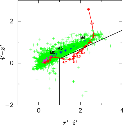
Figure 1.— Two color diagram of $r^{\prime}-i^{\prime}$ and $i^{\prime}-z^{\prime}$, that is used for our quasar selection. Green plus symbols denote point sources with $22<i^{\prime}({\tt MAG\_AUTO})<24$. Blue and magenta squares denote colors of M-type stars and K-type stars (Pickles 1998), respectively. The red line is the median track of the model quasar colors. The red error bars show the standard deviation of the $r^{\prime}-i^{\prime}$ and $i^{\prime}-z^{\prime}$ colors in our model quasar spectra. The black solid line shows our photometric criteria used to select quasar candidates at $z\sim 5$.

The 5$\sigma$ limiting AB apparent magnitudes are $u^{*}$ = 26.5, $g^{\prime}$ = 26.5, $r^{\prime}$ = 26.6, $i^{\prime}$ = 26.1, and $z^{\prime}$ = 25.1 ($3^{{}^{\prime\prime}}$ diameter aperture). Since we also use the Advanced Camera for Surveys (ACS) catalog (Koekemoer et al. 2007; Leauthaud et al. 2007) to separate galaxies from point sources, our survey area is restricted to the area mapped with ACS on HST ($1.64\ \rm deg^{2}$). Note that all of the data in the official COSMOS photometric redshift catalog overlaps the entire ACS field.

2.2. Quasar Candidate Selection

Table 1Properties of the quasar candidates at $z\sim 5$

Number			R.A.	Decl.	$i^{\prime}$ (MAG_AUTO)	$r^{\prime}-i^{\prime}$	$i^{\prime}-z^{\prime}$	$\rm Exp.Time^{a}$
			(deg)	(deg)	(mag)	(mag)	(mag)	(sec)
1			150.69131	1.637161	23.40	2.34	0.67	2400
2			150.45275	1.669653	23.48	2.04	2.69	3000
3			150.17448	1.629074	23.76	1.67	2.11	1800
4b			150.64917	1.816186	23.39	3.44	0.82	-
5			149.87082	1.882791	23.98	1.26	0.17	2400
6			149.85403	1.823611	23.97	2.58	0.87	2400
7			149.78245	2.221621	23.96	3.19	1.13	1800
8			149.69804	2.283260	23.67	2.04	0.44	1800
9			150.56861	2.317432	23.98	4.09	1.26	1800
10			150.05481	2.376726	23.89	1.09	0.25	2700
$11^{c}$			149.78381	2.452135	23.70	1.35	0.26	7200
12			150.16401	2.549605	23.31	1.96	0.61	2400
13			149.96443	2.473646	23.93	1.21	0.21	2700
14			150.66035	2.786445	23.51	1.93	0.57	2400
15			149.59161	2.659749	23.16	2.26	0.77	2400

Quasars at $z\sim 5$ show the Lyman break in their spectral energy distribution (SED) that falls between the wavelengths of the $r^{\prime}$ and $i^{\prime}$ filters, making their $r^{\prime}-i^{\prime}$ color redder than their $i^{\prime}-z^{\prime}$ color. We utilize this property to select candidates of low-luminosity quasars at $z\sim 5$. Here typical quasar colors as a function of redshift are necessary to define reliable color-selection criteria for quasars at $z\sim 5$. Therefore we generate model quasar spectra following the procedure generally adopted in previous studies (e.g., Fan 1999; Hunt et al. 2004; Richards et al. 2006; Siana et al. 2008), and derive the $g^{\prime}-r^{\prime}$, $r^{\prime}-i^{\prime}$, and $i^{\prime}-z^{\prime}$ colors of the model quasars at redshifts from 0 to 6. In this procedure, we adopt the typical power-law slope ($\alpha_{\nu}$ = 0.46, where $f_{\nu}\propto\nu^{-\alpha_{\nu}}$), Ly$\alpha$ rest-frame equivalent width ($\it EW_{\rm 0}$ = 90 Å), and typical emission-line flux ratios (Vanden Berk et al. 2001). The effects of the intergalactic absorption by the neutral hydrogen were corrected by adopting the extinction model of Madau (1995). Our simulated colors of the model quasars are shown in the $r^{\prime}-i^{\prime}$ versus $i^{\prime}-z^{\prime}$ diagram (Fig. 1). Note that the dispersions in the power-law slope and EWs of quasars are also taken into account when we calculate the photometric completeness of our survey (see Section 4).

We select our quasar photometric candidates at $z\sim 5$ using the following criteria:

$$22<i^{\prime}{\rm({\tt MAG\_AUTO})}<24,$$ (1)

$$i^{\prime}-z^{\prime}<0.45(r^{\prime}-i^{\prime})-0.24,$$ (2)

$$u^{*}>27.49,$$ (3)

$$g^{\prime}-r^{\prime}\geq 1.3,$$ (4)

and

$$r^{\prime}-i^{\prime}>1.0.$$ (5)

The criterion (2) is used to select quasars efficiently without significant contamination from stars (especially from M0 to M6, see also Fig. 1), taking the color distribution of stars and model quasars into account. To remove possible foreground contaminations further, we introduce the additional criteria (3), (4), and (5). These latter two color thresholds are adopted by taking empirical color distributions of quasars at $z\sim 5$ into account (Richards et al. 2006).

Here we comment on our point-source criterion based on the HST image (F814W, see Koekemoer et al. 2007), whose spatial resolution is $0\farcs 09$ in FWHM (that corresponds to $\sim 0.6\rm kpc$ at $z=5$). Since the size of high-$z$ quasar host galaxies is larger than 1 kpc (Targett et al. 2012), it is expected that the quasar host galaxies are spatially resolved in the ACS images. Therefore it would be possible some quasars could be excluded from the sample of our quasar photometric candidates. However, at $z\sim 1$, some earlier works show that the host galaxy of quasars with a similar absolute magnitude to our targets is typically $\sim 2$ mag fainter than their nucleus (e.g., McLeod & McLeod 2001; McLeod & Bechtold 2009). The brightness difference may be even larger at higher redshifts, because the typical Eddington ratio of luminous quasars is roughly constant at $z\sim 1-4$ (Trump et al. 2009) while the mass ratio of SMBHs to host galaxies is higher at higher redshifts (e.g., Treu et al. 2006; Woo et al. 2008, 2006; Merloni et al. 2010; Bennert et al. 2010, 2011). Therefore we conclude that quasars explored in this work should be recognized as point sources in the HST image. To distinguish the galaxies and point sources, Leauthaud et al. (2007) used the SExtractor parameter $\rm\tt MU\_MAX$ (peak surface brightness above the background level) and $\rm\tt MAG\_AUTO$ (see Fig. 5 of Leauthaud et al. 2007). Because the fact that the light distribution of a point source varies with magnitude. Therefore we can distinguish the extended objects and point sources by using the $\rm\tt MU\_MAX$ and the $\rm\tt MAG\_AUTO$.

Accordingly we removed 23 spatially-extended objects satisfying the criteria (1)–(5) based on the classification by Leauthaud et al. (2007). As a result, we obtain a sample of 15 quasar candidates among 7318 point sources with $22<i^{\prime}(\tt MAG\_AUTO)<\rm 24$. The selected candidates are listed in Table 1.

Figure 2.— Reduced spectrum of object No. 11 in Table 1 (upper panel) and typical sky spectrum (lower panel). Dotted lines show the expected wavelengths of quasar emission lines: Ly$\alpha$ $\lambda 1216$ and C iv $\lambda 1549$.

3. Spectroscopic Observation

The spectroscopic follow-up observations of the quasar candidates were carried out at the Subaru Telescope with the Faint Object Camera and Spectrograph (FOCAS; Kashikawa et al. 2002) on 7–11 January 2010. We used the 300 grating with the SO58 filter, whose wavelength coverage is 5800Å $\leq$ $\rm\lambda_{obs}$ $\leq$ 10000Å. We used a $0\farcs 8$-width slit, resulting in a wavelength resolution of $R\sim 700$ ($\Delta v$ $\sim 430$ km $\rm s^{-1}$) as measured by night sky emission lines. The typical seeing size was $\sim 0\farcs 7$. Due to the limited observing time, we observed 14 of the 15 candidates; the object No. 4 in Table 1 was not observed. The individual exposure time was 600 – 900 sec, and the total exposure time was 1800 – 7200 sec for each object.

Standard data reduction procedures were performed by using IRAF. After the sky subtraction, we extracted one-dimensional spectra with an aperture size of $1\farcs 8$ and the relative sensitivity calibration was performed using the spectral data of a spectrophotometric standard star, Feige 34. The spectra of 14 objects were then flux-calibrated using the $i^{\prime}$-band photometric magnitude of these objects. We found that one spectrum shows only narrow Ly$\alpha$ emission lines at $\lambda_{\rm obs}=7381$ Å($z\sim 5.07$ and $\Delta v_{\rm FWHM}\sim 800$ km $\rm s^{-1}$) without any high-ionization lines such as C iv (Fig. 2). Since this object is detected in the X-ray band by the Chandra-COSMOS survey (Elvis et al. 2009, CID-2220) and its X-ray luminosity is 3$\times$10⁴⁴ erg/s in the 2-10 keV rest frame band (Civano et al. 2011, 2012), it can be classified as an AGN. We can classify this object as a Type 2 AGN based on the upper limit available for the X-ray hardness ratio consistent with mild obscuration (NH$<$5$\times$10²³cm^-2) together with its Ly $\alpha$ spectral profile. Although the X-ray hardness ratio is not available for this object, we classify this object as a type-2 AGN based on its Ly$\alpha$ spectral profile. Therefore we conclude that no type-1 quasars are identified in our spectroscopic follow-up campaign. The spectra of the remaining 13 objects are consistent with those of Galactic late-type stars, and an example of these spectra is shown in Fig. 3.

4. Completeness

Quasar surveys are generally not perfectly complete due to various factors such as photometric errors and intrinsic variations in the spectra. Therefore, to derive the QLF acculately, the survey completeness needs to be estimated as a function of the quasar redshift and apparent magnitude. We derive the completeness by modeling quasar spectra, in a similar way as described in Section 2.2. Here we also take into account the intrinsic variation in the continuum slope and EWs of the emission lines. We assume a Gaussian distribution of the power-law slope $\alpha_{\nu}$ ($f_{\nu}\propto\nu^{-\alpha_{\nu}}$) and Ly$\alpha$ EWs, with means of 0.46 and 90Å (the same as those in Section 2.2), and a standard deviation of 0.30 and 20Å, respectively (Vanden Berk et al. 2001; Francis 1996; Hunt et al. 2004; Glikman et al. 2010). We include emission lines whose flux is larger than $0.5\%$ of the Ly$\alpha$ flux, given in Table 2 of Vanden Berk et al. (2001). The emission-line ratios are assumed to be the same for all model quasars (i.e., scaling to the Ly$\alpha$ strength). We also include the Balmer continuum and Fe ii features by using the template of Kawara et al. (1996). We create 1000 quasar spectra at each $\Delta$$z$ = 0.01 in the redshift range of $0<z<6$. The effects of intergalactic absorption by neutral hydrogen were corrected by adopting the extinction model of Madau (1995). Then, we calculated the colors of the model quasars in the observed frame. We compared the colors of the simulated quasars with the empirical quasar colors (SDSS DR7) to check whether the simulated quasar colors are consistent with the empirical quasar colors. Fig. 4 shows the comparison between the empirical and simulated quasar colors of $g^{*}-r^{*}$, $r^{*}-i^{*}$, and $i^{*}-z^{*}$ by using the transmission curves of the SDSS filters. Note that the dispersion of the simulated quasar colors is systematically smaller than the dispersion of the observed quasar colors, through the average color is consistent between the simulated and observed quasar colors. This is because the simulated colors presented here do not take photometric errors into account. The photometric errors are properly taken into account when the completeness is calculated, as described below.

Figure 3.— Example of the late type star spectrum (upper panel; No. 2 in Table 1) and typical sky spectrum (lower panel).

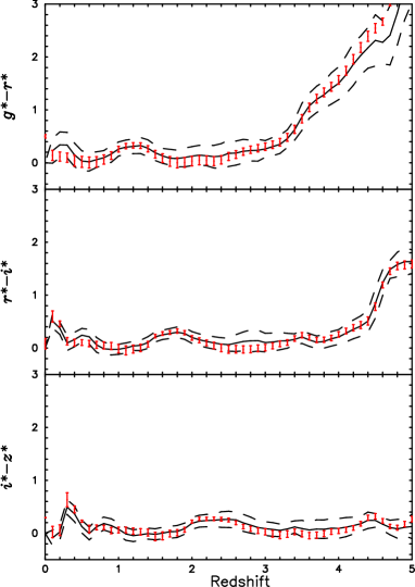
Figure 4.— Comparison between the empirical and simulated quasar colors. Solid black lines show the empirical mean colors of the SDSS DR7 quasars. Dashed black lines show 1 sigma dispersions of the SDSS DR7 quasar colors. Red points show the simulated quasar colors. Red vertical lines show the standard deviation of simulated quasar colors which do not include photometric errors.

To estimate the photometric completeness, we put the 1000 model quasars at each grid point in apparent magnitude and redshift into Subaru Suprime-Cam FITS images as point sources, using the IRAF mkobjects task in the artdata package. As for 1000 model quasars, they were generated on a Monte Carlo method of drawing a value of alpha and EW. These point sources have apparent magnitudes calculated from their simulated spectra, in each image ($g^{\prime}$, $r^{\prime}$, $i^{\prime}$, and $z^{\prime}$). We then tried to detect them in the $i^{\prime}$-band image with SExtractor, and measure their colors in the double-image mode. Note that the measured apparent magnitudes and colors of the simulated quasars are generally different from the magnitudes and colors before inserted into the Suprime-Cam images, due to the effects of photometric errors and neighboring foreground objects. Accordingly, some model quasars are not selected as photometric candidates of quasar with the criteria (1) – (5). To calculate the fraction of model quasars that are selected as photometric candidates in the above process, we estimate the photometric completeness at various magnitudes and redshifts (Fig. 5). The redshift range of the inferred completeness is moderately high at 4.5 $\lesssim$ z $\lesssim$ 5.5. More specifically, the inferred completeness is $\sim 90\%$ for quasars with $i^{\prime}=22.5$, and $\sim 80\%$ for those with $i^{\prime}=23.5$ in that redshift range. The small dip at $z\sim 5.2-5.3$ in the estimated completeness is due to the C iv emission that causes the $i^{\prime}-z^{\prime}$ color to be red at that redshift range.

5. Quasar Luminosity Function

To calculate the upper limits of the quasar space density, we compute the effective comoving volume of the survey as:

$$V_{\rm eff}(m_{i^{\prime}})=d\Omega\int_{z=0}^{z=\infty}C(m_{i^{\prime}},z)\frac{dV}{dz}dz,$$ (6)

where $d\Omega$ is the solid angle of the survey and $C(m_{i^{\prime}},z)$ is the photometric completeness derived in Section 4. For comparison with other works, we convert the $i^{\prime}$-band apparent magnitude to the absolute AB magnitude at 1450Å (e.g., Richards et al. 2006; Croom et al. 2009; Glikman et al. 2010):

$$M_{1450}=m_{i^{\prime}}+5-5{\rm log}d_{L}(z)+2.5(1-\alpha_{\nu})$$

$${\rm log}(1+z)+2.5\alpha_{\nu}{\rm log}\left(\frac{\lambda_{i^{\prime}}}{1450\rm\AA}\right),$$ (7)

where $d_{L}(z)$, $\alpha_{\nu}$, and $\lambda_{i^{\prime}}$ are the luminosity distance, spectral index of the quasar continuum ($f_{\nu}\propto\nu^{-\alpha_{\nu}}$), and the effective wavelength of the $i^{\prime}$-band ($\lambda_{i^{\prime}}$=7684$\rm\AA$), respectively. We assumed the $\alpha_{\nu}=0.46$ when we used the equation (7). As for the quasar candidates which did not perform the spectroscopic observations, we calculated the absolute magnitude at 1450$\rm\AA$ by assuming the effective redshift. Given the effective comoving volume, the 1 $\sigma$ confidence upper limits on the space density of type-1 quasars are calculated using statistics from Gehrels (1986).

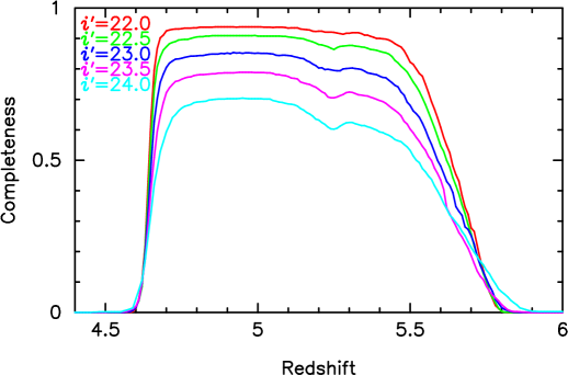
Figure 5.— Simulated photometric completeness. Red, green, blue, purple, and cyan lines show the completeness for quasars with $m_{i^{\prime}}$ = 22.0, 22.5, 23.0, 23.5, and 24.0, respectively.

The derived 1 $\sigma$ confidence upper limits on the space density of type-1 quasars are $\Phi<$ 1.33 $\times$ 10^-7 Mpc^-3 mag^-1 for $-24.52<M_{1450}<-23.52$ and $\Phi<$ 2.88 $\times$ 10^-7 Mpc^-3 mag^-1 for $-23.52<M_{1450}<-22.52$. Note that there is another quasar candidate in the magnitude bin of $-23.52<M_{1450}<-22.52$ which was not observed with FOCAS. We take into account the possibility that this candidate is a quasar when calculating the $1\sigma$ confidence upper limit on the space density of type-1 quasars for $-23.52<M_{1450}<-22.52$. The obtained 1 $\sigma$ confidence upper limits on the space density of type-1 quasars are plotted in Fig. 6.

To compare our upper limits on the quasar space density with the previous quasar surveys at similar redshifts, we also plot the results of COMBO-17 (Wolf et al. 2003), SDSS (Richards et al. 2006), and GOODS (Fontanot et al. 2007), in the redshift ranges of 4.2 $<$ ${\it z}$ $<$ 4.8, 4.5 $<$ ${\it z}$ $<$ 5.0, and 4.0 $<$ ${\it z}$ $<$ 5.2 respectively, in Fig. 6. Note that the low-luminosity quasar sample of Fontanot et al. (2007) includes type-2 quasars while our sample and the sample of Wolf et al. (2003) do not include type-2 quasars. To compare the result of Fontanot et al. (2007), we also calculated the quasar space density when we included a type-2 quasar and the obtained quasar space density and its error are $\Phi=$ $0.87_{-0.72}^{+2.01}$ $\times$ 10^-7 Mpc^-3 mag^-1 for $-23.52<M_{1450}<-22.52$ (see Fig. 6). This figure shows a marginal discrepancy between the results of Fontanot et al. (2007) and of ours. However, the redshift difference between the two studies should be taken into account for such a comparison because the quasar space density shows significant redshift evolution.

The $z\sim 5$ quasar luminosity functions. The red filed squares show our results (1$\sigma$ confidence limits on the quasar space density) and the red open square shows the quasar space density when we include a type-2 quasar at $z\sim 5.07$. For clarifying the data plots in the figure, the open red square is slightly shifted to the left direction to avoid the overlap of the error bars. Triangles, squares, and circles denote the results reported by Fontanot et al. (2007), Richards et al. (2006), and Wolf et al. (2003), respectively.

In Fig. 7, we plot the QLF reported by Fontanot et al. (2007) after correcting for the redshift difference (i.e., taking the redshift evolution in the QLF into account), adopting the model 13a in Fontanot et al. (2007). The model 13a assumes a pure density evolution of the QLF with an exponential form, that gives the minimum $\chi^{2}$ among the models examined in Fontanot et al. (2007). More specifically, in the model 13a, the bright-end slope is fixed to be 3.31 and there are three free parameters; are the faint-end slope, normalization, and redshift evolution parameter. Fig. 7 shows that our quasar space density at $z\sim 5$ are higher than the result of Fontanot et al. (2007) and thus our results are not contradictory to their result, once the redshift difference is corrected. Here it should be mentioned that Fontanot et al. (2007) adopted a different method in deriving the photometric completeness from other surveys, that may introduce a possible systematic difference from other studies (see also Glikman et al. 2010). This effect is seen in Fig. 6, where the inferred bright-end quasar space density is different between the results by Fontanot et al. (2007) and by Richards et al. (2006) even although the same SDSS quasar sample is used in the two studies. This suggests that the completeness adopted in Fontanot et al. (2007) may be underestimated, and accordingly the quasar space density is possibly overestimated by a factor of $\sim 2-3$. In the case that we derive the faint end of the QLF at $z\sim 5$ by using the completeness which is calculated by Richards et al. (2006), the QLF of Fontanot et al. (2007) shifts toward lower space density in Fig. 7, i.e., well below our upper limits.

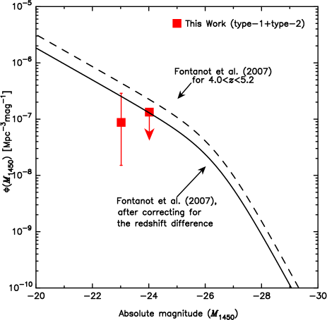
Figure 6.— Comparison of $z\sim 5$ quasar luminosity functions when we include a type-2 quasar at $z\sim 5.07$. The red squares show our results when we include a type-2 quasar at $z\sim 5.07$. The black dashed and solid lines are the QLF reported by Fontanot et al. (2007), before and after correcting for the redshift difference between their study and ours (assuming pure density evolution, see the main text for details).

In order to constrain the faint end of the QLF at $z\sim 5$ quantitatively, we search for parameter values that satisfy our result. Here we adopt the following double power-law function:

$$\Phi(M_{1450},z)=\hskip 156.49014pt$$

$$\frac{\Phi(M^{*}_{1450})}{10^{0.4(\alpha+1)(M_{1450}-M^{*}_{1450})}+10^{0.4(\beta+1)(M_{1450}-M^{*}_{1450})}},$$ (8)

where $\alpha$, $\beta$, $\Phi(M^{*}_{1450})$, and $M^{*}_{1450}$ are the bright-end slope, the faint-end slope, the normalization of the luminosity function, and the characteristic absolute magnitude, respectively. Among the four parameters, the bright-end slope ($\alpha$) is fixed to be $\alpha=-3.31$ based on the SDSS results (see Fontanot et al. 2007). The parameter ranges which satisfy our results are shown in Fig. 8. Note that it is important to examine the redshift evolution of the faint-end slope and break magnitude, because such parameters give us useful constraints on the evolutionary model of SMBHs and quasars (e.g., Hopkins et al. 2006, 2007). By taking into account of the results obtained in COSMOS for $z\sim 5$, the break magnitude in the QLF is brighter than $M^{*}_{\rm 1450}\sim-26$ at $z\sim 5$. This is significantly brighter than the QLF break magnitude for $z\sim 4$ reported by Ikeda et al. (2011) and Glikman et al. (2011), as shown in Fig. 8. A possible explanation for this evolution is that the mass accretion in most quasars at $z\sim 5$ is higher than at $z\sim 4$ (although the quasar number density is lower at $z\sim 5$), which makes the characteristic magnitude brighter at $z\sim 5$ than at $z\sim 4$.

Figure 7.— Constraints on the faint-end slope $\beta$ and the break magnitude $M_{\rm 1450}^{*}$. The shaded region shows the parameter space that is consistent with the inferred 1$\sigma$ confidence upper limits on the quasar space density at $z\sim 5$ derived in our study. A dot and triangle are the results inferred at $z\sim 4$ by Ikeda et al. (2011) and Glikman et al. (2011), respectively. Note that we estimate the errors of $M^{*}_{\rm 1450}$ and the faint-end slope by applying a weighted least-squares method while Glikman et al. (2011) estimated them by applying the STY maximum-likelihood method (Efstathiou et al. 1988).

Here we discuss the evolution of the quasar space density in the context of the AGN downsizing. The evolution of the quasar space density for different absolute magnitude bins provides important information to constrain the evolution of SMBHs. Therefore we plot the quasar space density for different absolute magnitude bins as a function of redshift in Fig. 9. Although there are a number of low-luminosity quasar surveys at $z\sim 3$ (Wolf et al. 2003; Hunt et al. 2004; Fontanot et al. 2007; Bongiorno et al. 2007), we plot only the results of the 2dF-SDSS LRG and Quasar Survey (2SLAQ; Croom et al. 2009), the Spitzer Wide-area Infrared Extragalactic Legacy Survey (SWIRE; Siana et al. 2008), and SDSS (Richards et al. 2006), in order to avoid data with large statistical errors. While most studies at $z<3$ suggest consistent results (i.e., the AGN downsizing), the situation is rather controversial at $z>3$. Recently, the new $z\sim 4$ QLF results of the NOAO Deep Wide-Field Survey (NDWFS) and the Deep Lens Survey (DLS) are reported by Glikman et al. (2011). Interestingly, the results of Glikman et al. (2011) suggest constant or higher number densities of low-luminosity QSOs at $z>3$, while our COSMOS result suggests a continuous decrease of these objects from $z\sim 2$ to $z\sim 5$.

Our result is consistent with the downsizing AGN evolution suggested by previous quasar surveys at lower-$z$ both in the optical and X-ray (e.g., Croom et al. 2009; Ueda et al. 2003; Hasinger et al. 2005). Willott et al. (2010) reported the faint end of the QLF at $z\sim 6$ although there is a large error bar for the faintest magnitude bin because only one quasar was found. The $z\sim 6$ space density at $M_{\rm 1450}\sim-22$ is lower than the upper limit of our $z\sim 5$ space density at the same magnitude and this result is also consistent with the AGN downsizing evolution. However, the results of Glikman et al. (2011) require a different picture at $z>3$, being inconsistent with the downsizing scenario. It is not obvious what is causing this discrepancy. Masters et al. (submitted to the ApJ) stated that cosmic variance cannot be responsible for the observed discrepancy in space density of low-luminosity quasars between the COSMOS and the DLS NDWFS fields. If this discrepancy is due to the difference in the quasar selection criteria, then this discrepancy could be caused by the presence or absence of the point source selection on the HST images. However, both Ikeda et al. (2011) and Glikman et al. (2011) obtained the spectra of most quasar candidates to remove the contaminations. Consequently, we cannot explain this discrepancy due to the difference of the quasar selection criteria. Therefore it remains important that we search for low-luminosity quasars at high redshift in other fields and derive the faint end of the QLF. We also plot the quasar space density measured in the GOODS fields (Fontanot et al. 2007) in Fig. 9, which is consistent with both results from Glikman et al. (2011) and COSMOS due to its large uncertainty. Further observations of low-luminosity quasars in a wider survey area are crucial to derive firm constraints on the scenarios of the quasar evolution, especially at $z>4$.

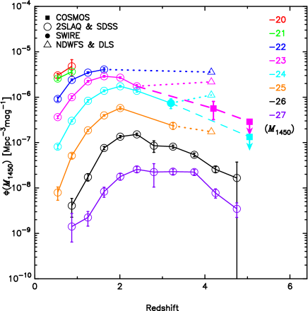
Figure 8.— The redshift evolution of the quasar space density. Red, green, blue, magenta, light blue, orange, black, purple lines are the space density of quasars with $M_{1450}=-20,-21,-22,-23,-24,-25,-26$, and $-27$, respectively. Filled squares, open circles, filled circle, and open triangles denote the results of different quasar surveys, as described in the upper-left side of the panel (see the main text for details). For the comparison, the results of COSMOS and previous surveys are connected by the dashed lines while the results of NDWFS $\&$ DLS (Glikman et al. 2011) are connected by the dotted lines.

6. Summary

In order to examine the faint end of the QLF at $z\sim 5$, we select photometric candidates of quasars at $z\sim 5$ in the COSMOS field. The main results of this study are:

• Although we discover the type-2 quasar at $z\sim 5.07$, no type-1 quasars at $z\sim 5$ are identified through the follow-up spectroscopic observation.

• The upper limits on the type-1 quasar space density are $\Phi<$ 1.33 $\times$ 10^-7 Mpc^-3 mag^-1 for $-24.52<M_{1450}<-23.52$ and $\Phi<$ 2.88 $\times$ 10^-7 Mpc^-3 mag^-1 for $-23.52<M_{1450}<-22.52$.

• The quasar space density and its error when we include a type-2 quasar at $z\sim 5.07$ are $\Phi=$ $0.87_{-0.72}^{+2.01}$ $\times$ 10^-7 Mpc^-3 mag^-1 for $-23.52<M_{1450}<-22.52$.

• The derived upper limits on the quasar space density are consistent with the QLF inferred by the previous works at $z\sim 5$.

• The characteristic absolute magnitude of the QLF shows a significant redshift evolution between $z\sim 4$ ($M^{*}_{1450}>-26$) and $z\sim 5$ ($M^{*}_{1450}<-26$).

• A continuous decrease of the space density of low-luminosity ($-24\lesssim M_{1450}\lesssim-23$) quasars is inferred, that is roughly consistent with the picture of the AGN downsizing evolution.

References

- Bennert et al. (2011) Bennert, V. N., Auger, M. W., Treu, T., Woo, J.-H., & Malkan, M. A. 2011, ApJ, 742, 107
- Bennert et al. (2010) Bennert, V. N., Treu, T., Woo, J.-H., et al. 2010, ApJ, 708, 1507
- Bertin & Arnouts (1996) Bertin, E., & Arnouts, S. 1996, A&AS, 117, 393
- Bongiorno et al. (2007) Bongiorno, A., Zamorani, G., Gavignaud, I., et al. 2007, A&A, 472, 443
- Boulade et al. (2003) Boulade, O., Charlot, X., Abbon, P., et al. 2003, in Society of Photo-Optical Instrumentation Engineers (SPIE) Conference Series, Vol. 4841, Society of Photo-Optical Instrumentation Engineers (SPIE) Conference Series, ed. M. Iye & A. F. M. Moorwood, 72–81
- Boyle et al. (1988) Boyle, B. J., Shanks, T., & Peterson, B. A. 1988, MNRAS, 235, 935
- Brusa et al. (2009) Brusa, M., Comastri, A., Gilli, R., et al. 2009, ApJ, 693, 8
- Capak et al. (2007) Capak, P., Aussel, H., Ajiki, M., et al. 2007, ApJS, 172, 99
- Civano et al. (2011) Civano, F., Brusa, M., Comastri, A., et al. 2011, ApJ, 741, 91
- Civano et al. (2012) Civano, F., Elvis, M., Brusa, M., et al. 2012, ArXiv e-prints
- Cool et al. (2006) Cool, R. J., Kochanek, C. S., Eisenstein, D. J., et al. 2006, AJ, 132, 823
- Croom et al. (2009) Croom, S. M., Richards, G. T., Shanks, T., et al. 2009, MNRAS, 399, 1755
- Efstathiou et al. (1988) Efstathiou, G., Ellis, R. S., & Peterson, B. A. 1988, MNRAS, 232, 431
- Elvis et al. (2009) Elvis, M., Civano, F., Vignali, C., et al. 2009, ApJS, 184, 158
- Enoki et al. (2003) Enoki, M., Nagashima, M., & Gouda, N. 2003, PASJ, 55, 133
- Fan (1999) Fan, X. 1999, AJ, 117, 2528
- Fan et al. (2006) Fan, X., Strauss, M. A., Richards, G. T., et al. 2006, AJ, 131, 1203
- Fanidakis et al. (2012) Fanidakis, N., Baugh, C. M., Benson, A. J., et al. 2012, MNRAS, 419, 2797
- Fontanot et al. (2007) Fontanot, F., Cristiani, S., Monaco, P., et al. 2007, A&A, 461, 39
- Francis (1996) Francis, P. J. 1996, PASA, 13, 212
- Gehrels (1986) Gehrels, N. 1986, ApJ, 303, 336
- Glikman et al. (2010) Glikman, E., Bogosavljević, M., Djorgovski, S. G., et al. 2010, ApJ, 710, 1498
- Glikman et al. (2011) Glikman, E., Djorgovski, S. G., Stern, D., et al. 2011, ApJ, 728, L26
- Goto (2006) Goto, T. 2006, MNRAS, 371, 769
- Gültekin et al. (2009) Gültekin, K., Richstone, D. O., Gebhardt, K., et al. 2009, ApJ, 698, 198
- Häring & Rix (2004) Häring, N., & Rix, H.-W. 2004, ApJ, 604, L89
- Hasinger et al. (2005) Hasinger, G., Miyaji, T., & Schmidt, M. 2005, A&A, 441, 417
- Hopkins et al. (2006) Hopkins, P. F., Hernquist, L., Cox, T. J., et al. 2006, ApJ, 639, 700
- Hopkins et al. (2007) Hopkins, P. F., Richards, G. T., & Hernquist, L. 2007, ApJ, 654, 731
- Hunt et al. (2004) Hunt, M. P., Steidel, C. C., Adelberger, K. L., & Shapley, A. E. 2004, ApJ, 605, 625
- Ikeda et al. (2011) Ikeda, H., Nagao, T., Matsuoka, K., et al. 2011, ApJ, 728, L25
- Ilbert et al. (2009) Ilbert, O., Capak, P., Salvato, M., et al. 2009, ApJ, 690, 1236
- Jiang et al. (2008) Jiang, L., Fan, X., Annis, J., et al. 2008, AJ, 135, 1057
- Jiang et al. (2009) Jiang, L., Fan, X., Bian, F., et al. 2009, AJ, 138, 305
- Kashikawa et al. (2002) Kashikawa, N., Aoki, K., Asai, R., et al. 2002, PASJ, 54, 819
- Kawara et al. (1996) Kawara, K., Murayama, T., Taniguchi, Y., & Arimoto, N. 1996, ApJ, 470, L85
- Koekemoer et al. (2007) Koekemoer, A. M., Aussel, H., Calzetti, D., et al. 2007, ApJS, 172, 196
- Lawrence et al. (2007) Lawrence, A., Warren, S. J., Almaini, O., et al. 2007, MNRAS, 379, 1599
- Leauthaud et al. (2007) Leauthaud, A., Massey, R., Kneib, J.-P., et al. 2007, ApJS, 172, 219
- Madau (1995) Madau, P. 1995, ApJ, 441, 18
- Mahabal et al. (2005) Mahabal, A., Stern, D., Bogosavljević, M., Djorgovski, S. G., & Thompson, D. 2005, ApJ, 634, L9
- Marconi & Hunt (2003) Marconi, A., & Hunt, L. K. 2003, ApJ, 589, L21
- McLeod & Bechtold (2009) McLeod, K. K., & Bechtold, J. 2009, ApJ, 704, 415
- McLeod & McLeod (2001) McLeod, K. K., & McLeod, B. A. 2001, ApJ, 546, 782
- Merloni et al. (2010) Merloni, A., Bongiorno, A., Bolzonella, M., et al. 2010, ApJ, 708, 137
- Miyazaki et al. (2002) Miyazaki, S., Komiyama, Y., Sekiguchi, M., et al. 2002, PASJ, 54, 833
- Mortlock et al. (2011) Mortlock, D. J., Warren, S. J., Venemans, B. P., et al. 2011, Nature, 474, 616
- Pei (1995) Pei, Y. C. 1995, ApJ, 438, 623
- Pickles (1998) Pickles, A. J. 1998, PASP, 110, 863
- Richards et al. (2006) Richards, G. T., Strauss, M. A., Fan, X., et al. 2006, AJ, 131, 2766
- Scoville et al. (2007) Scoville, N., Aussel, H., Brusa, M., et al. 2007, ApJS, 172, 1
- Siana et al. (2008) Siana, B., Polletta, M. d. C., Smith, H. E., et al. 2008, ApJ, 675, 49
- Taniguchi et al. (2007) Taniguchi, Y., Scoville, N., Murayama, T., et al. 2007, ApJS, 172, 9
- Targett et al. (2012) Targett, T. A., Dunlop, J. S., & McLure, R. J. 2012, MNRAS, 420, 3621
- Treu et al. (2006) Treu, T., Koopmans, L. V., Bolton, A. S., Burles, S., & Moustakas, L. A. 2006, ApJ, 640, 662
- Trump et al. (2009) Trump, J. R., Impey, C. D., Kelly, B. C., et al. 2009, ApJ, 700, 49
- Trump et al. (2011) —. 2011, ApJ, 733, 60
- Ueda et al. (2003) Ueda, Y., Akiyama, M., Ohta, K., & Miyaji, T. 2003, ApJ, 598, 886
- Vanden Berk et al. (2001) Vanden Berk, D. E., Richards, G. T., Bauer, A., et al. 2001, AJ, 122, 549
- Willott et al. (2007) Willott, C. J., Delorme, P., Omont, A., et al. 2007, AJ, 134, 2435
- Willott et al. (2009) Willott, C. J., Delorme, P., Reylé, C., et al. 2009, AJ, 137, 3541
- Willott et al. (2010) —. 2010, AJ, 139, 906
- Wolf et al. (2003) Wolf, C., Wisotzki, L., Borch, A., et al. 2003, A&A, 408, 499
- Woo et al. (2006) Woo, J.-H., Treu, T., Malkan, M. A., & Blandford, R. D. 2006, ApJ, 645, 900
- Woo et al. (2008) —. 2008, ApJ, 681, 925