Modeling the physical and excitation conditions of the molecular envelope of NGC 7027

Abstract

Context. The link between the shaping of bipolar planetary nebulae and the mass ejection activity of their central stars is still poorly understood. Appropriately characterizing the evolution of the shells ejected during the late stages of stellar evolution and the interaction between these shells is fundamental to gain insight into the mechanism of nebular shaping. This must include the study of the molecular emission, which tracks the mass-loss history during the late AGB and post-AGB stages, when the nebula is being actively shaped.

Aims. Herschel/HIFI provides an invaluable tool by opening a new window (most of the sub-mm and far infrared range is only accessible from space) from which to probe warm molecular gas ($\sim$50–1000 K). This paper presents a radiative-transfer, spatio-kinematic modeling of the molecular envelope of the young planetary nebula NGC 7027 in several high- and low$-J$ ¹²CO and ¹³CO transitions observed by Herschel/HIFI and the IRAM 30-m radio-telescope, and discusses the structure and dynamics of the molecular envelope.

Methods. We have developed a code which, used along with the existing SHAPE software (Steffen et al., 2011), implements spatio-kinematic modeling with accurate non-LTE calculations of line excitation and radiative transfer in molecular species. We have used this code to build a relatively simple “russian doll” model to account for the physical and excitation conditions of the molecular envelope of NGC 7027.

Results. The model nebula consists of four nested, mildly bipolar shells plus a pair of high-velocity blobs. The innermost shell is the thinnest and shows a significant jump in physical conditions (temperature, density, abundance and velocity) with respect to the adjacent shell. This is a clear indication of a shock front in the system, which may have played a role in the shaping of the nebula. Each of the high-velocity blobs is divided into two sections with considerably different physical conditions. The striking presence of H₂O in NGC 7027, a C-rich nebula, is likely due to photo-induced chemistry from the hot central star, although formation of water by shocks cannot be ruled out. The computed molecular mass of the nebula is 1.3 M_⊙, compatible with that derived from previous works.

1 Introduction

The physical mechanisms behind the shaping of proto-planetary nebulae (PPNe) and young planetary nebulae (PNe) has been and still is a subject of intense debate (see e.g. Balick & Frank, 2002). In particular, PPNe and young PNe usually show high-velocity outflows, usually in the polar directions, along with slower components whose velocities are comparable to those of the winds of AGB envelopes. These fast-bipolar outflows are thought to be the result of the propagation of shocks in the polar regions of the dense AGB shell during the evolution towards PPNe. However, many aspects of this process are poorly understood at present.

Tracking the mass ejecta of planetary nebulae (PNe) and proto-planetary nebulae (PPNe) by means of molecular emission lines can provide crucial clues for better understanding this topic. Herschel/HIFI provides an invaluable tool, as it probes warm molecular gas ($\sim$50–1000 K) by producing high-resolution spectra in high-excitation transitions (e.g. ¹²CO $J$=6$-$5, 10$-$9 and 16$-$15), some of which are unobservable from the ground, rendering ground-based telescopes esentially useless to accurately probe molecular gas with temperatures over $\sim$100 K.

Recently, as part of the guaranteed-time key program HIFISTARS, a sample of ten PPNe and young PNe were observed with Herschel/HIFI (Bujarrabal et al., 2012). Although HIFISTARS only includes observations towards the center of these nebulae, the kinematics and the excitation conditions of the warm molecular gas of the target can be studied with unprecedented detail thanks to the high spectral resolution of the profiles.

This work focuses on one of the targets observed within the HIFISTARS program, NGC 7027 (PN G084.9-03.4). With a kinematical age of just 600 years (based on its radio flux, see Masson 1989) and located at 1 kpc (Zijlstra et al., 2008), this compact and young PNe is one of the brightest nebulae in the sky and the most extensively studied PNe so far. NGC 7027 is a carbon-rich nebula with a very high-excitation spectrum (e.g. it shows ion lines such as O iv and Mg v). It hosts one of the hottest central stars known to date, with a T${}_{\mathrm{eff}}\sim$200,000 K (e.g Latter et al., 2000). A small, essentially ellipsoidal, expanding ionized shell surrounds the central star (Masson, 1989). Further outwards, a thin H₂ shell indicates the presence of a photo-dissociation region (PDR) and shows signs of recent interaction with collimated outflows (Cox et al., 2002). The nebula also shows molecular emission from CO beyond the PDR, extending further out to 15-20 arcsec from the central star. In particular, Nakashima et al. (2010) carried out interferometric observations in the CO $J$=2$-$1 and 1$-$0 lines and found that the CO envelope could be roughly modeled as an ellipsoidal shell, despite some deviations caused by a high-velocity component. The kinematics of this cold, molecular envelope seems to be closely linked with that of the inner ionized shell and the PDR (Cox et al., 1997, Latter et al., 2000).

The amount of molecular mass inferred from the CO emission is very significant. In fact, despite hosting one of the hottest central stars known, the ionized mass only represents 2% of the total measured mass of the nebula, 1.4 M_⊙, while the vast majority of the nebula (85%) consists of molecular gas, the remaining 13% being in the form of neutral atomic gas (Fong et al., 2001). It seems clear that any approach towards understanding the shaping mechanism of this nebula must take into account the emission from molecular gas.

In this work, we present a detailed study of the molecular envelope of NGC 7027, combining observational data from low-$J$ transitions, observed with the IRAM 30-m radio-telescope with data from high-$J$, observed as part of the HIFISTARS program. We have developed a code, shapemol, which, used along with SHAPE (Steffen et al., 2011), implements spatio-kinematic modeling with accurate calculations of non-LTE line excitations and radiative transfer in molecular species. The high quality of the HIFI data, together with shapemol, have allowed us to study, for the first time in such level of detail, the kinematics and excitation conditions of the warm, molecular (CO-rich) gas of a PN.

A preliminar version of this work was reported in Santander-Garcia et al. (2011).

2 Observations

The observations used in this paper (see Fig. 1) for the modeling of the molecular envelope of NGC 7027 have been already presented by Bujarrabal et al. (2001), ¹²CO and ¹³CO $J$=1$-$0 and 2$-$1 data, and Bujarrabal et al. (2012), rest of the data consisting of the high-$J$ transitions. Here we will briefly summarize the main observational characteristics of the data (see Table 1), as they have been described in full detail in these papers. CO $J$=1$-$0 and 2$-$1 spectra were obtained in 1999 and 2000 using the IRAM 30-m at Pico de Veleta (Spain). This is a very well characterized ground-based instrument, in which the main source of uncertainty in the absolute calibration of the data comes from the correction for the opacity of the atmosphere. Although this effect is measured every 20 to 30 min, in standard conditions we cannot guarantee accuracies better than 20–25% when comparing data from Pico de Veleta with those from other telescopes, as this is the best accuracy our group has found on long-term observations of the same standard sources, specially for observations dating a decade or more. Spectra at higher frequencies are taken from the Herschel/HIFI HIFISTARS GTKP (P.I. V. Bujarrabal). In this case, the main source or uncertainty in the absolute calibration of the data of this space-based telescope comes from the fact that the gain ratio between the two sidebands of the receivers is not well known. For the HIFISTARS data we have adopted uncertainty values from 15% to 30% depending on the receiver band, following the description of the HIFI instrument characteristics and performances given by Roelfsema et al. (2012). In all cases we have used the $T_{\mathrm{mb}}$ intensity scale, that can be directly compared with the model results when these take into account the shape of the beam of the telescope (see below).

In all cases, the spectra are taken towards the central star, located at J2000 R.A. 21^h07^m01^s.59 Dec.$+$42^∘14^′10.^′′2. The nebula is sometimes larger than the beam of the telescope (12–22 arcsec for the 30-m, and 12–33 arcsec for HIFI), and therefore by observing just the central position we do not observe its full emission. This is particularly true for the higher frequencies in both telescopes (at 220–230 GHz for IRAM 30-m and 1800 GHz for Herschel/HIFI), but this effect has been properly taken into account in our modeling (see section 4). For this purpose we have assumed that the telescope beam shape is well represented by a symmetrical 2D-Gaussian solely characterized by its FWHP, what has been taken to be equal to the measured HPBW of the two instruments at the corresponding frequencies (see Table 1).

The spectral resolution of the instruments is also limited. For the IRAM 30-m observations, the data were taken from the (now decommissioned) 100 kHz filter-bank, after degrading the resolution to 300 kHz by averaging every three channels, resulting in velocity resolutions of 0.8–0.9 km s^-1 for the 1–0 lines, and of 0.4 km s^-1 for the 2–1 lines. For the Herschel/HIFI data, we have used the Wide Band Spectrometer (WBS) in standard configuration, providing a spectral resolution of about 1.1 MHz, slightly varying across the observed band. The data have been oversampled in a homogeneous 0.5 MHz spectral channels, that we have degraded down to resolutions equivalent to 0.4 to 1.6 km s^-1) depending of the strength of the detected line and the required S/N ratio.

Table 1: Observing log and profile features.

Species	Transition	Frequency	Resolution	Tmb peak†	r.m.s.	Integ. flux⋆	HPBW
		(GHz)	(km s-1)	(K)	(K)	(K km s-1)	(′′)
IRAM 30-m observationsa
12CO	$J$=1$-$0	115.271	0.8	11.9	7.7$\times$10-2	332	22
12CO	$J$=2$-$1	230.538	0.4	30.9	9.9$\times$10-2	667	12
13CO	$J$=1$-$0	110.201	0.9	0.3	9.4$\times$10-3	7.9	22
13CO	$J$=2$-$1	220.399	0.4	1.3	3.0$\times$10-2	31	12
Herschel/HIFI observationsb
12CO	$J$=6$-$5	691.473	0.4	5.1	1.3$\times$10-2	137	31
12CO	$J$=10$-$9	1151.985	0.4	5.5	5.5$\times$10-2	146	20
12CO	$J$=16$-$15	1841.346	0.5	2.5	9.3$\times$10-2	52	12
13CO	$J$=6$-$5	661.067	0.5	0.3	8.6$\times$10-3	8.3	31
13CO	$J$=10$-$9	1101.350	0.5	0.2	2.5$\times$10-2	5.7	20
C18O	$J$=6$-$5	658.506	0.9	0.03	6.1$\times$10-3	0.7	33
OH	${}^{2}\Pi_{1/2}$ $J$=3/2--1/2+	1834.75	1.6	0.16	4.8$\times$10-2	6.3	12
p-H2O	$J_{K_{a},K_{c}}$=$1_{1,1}-0_{0,0}$	1113.343	0.9	0.1	1.9$\times$10-2	2.1	20
o-H2O	$J_{K_{a},K_{c}}$=$1_{1,0}-1_{0,1}$	556.936	0.5	0.1	5.5$\times$10-3	2.1	39

Notes:
^†Maximum intensity of the profile in main beam temperature $T_{\mathrm{mb}}$(K), defined as the peak intensity minus the r.m.s. in the spectrum
^⋆Integrated flux of the profile.
^a Observations published in Bujarrabal et al. (2001)
^b Observations published in Bujarrabal et al. (2012)

3 Modeling

The main goal of our modeling is to determine the physical conditions (densities, temperatures and abundances) and the general kinematic structure of the nebula. Note that an accurate determination of the 3-D structure from our data is prevented by the lack of spatial resolution. In fact, the only information about the spatial structure is concealed in the frequency-dependent beam size, which weighs the emission from the central region and that coming from the outer region in a different fashion for each transition, and which is, for the highest-$J$ transitions, smaller than the molecular CO shell at lower-$J$ described by previous works (see beam size column in Table 1). Hence, the general geometry of the nebula has been deduced both from the analysis of previous works and a series of reasonable deductions from the Herschel and IRAM data-set (see section 4.1). In any case, the following model should be considered as a first, simplified approach to a much more complex reality.

The modeling process is similar to standard spatio-kinematic modeling (e.g. Santander-García et al., 2004), except that it incorporates full radiative-transfer solving for different transitions, creating synthetic profiles to be matched against the observations. We have achieved this by using a special version (4.51$\beta$) of the SHAPE software by Steffen et al. (2011), specifically customized for usage alongside our own GDL/IDL-based code, shapemol.

SHAPE is a software tool for building spatio-kinematic models of nebulae. It allows to easily implement a 3-D structure and 3-D velocity field to describe the model nebula, and generate synthetic images, position-velocity diagrams and/or channel maps for direct comparison with observations. Its versatility has made it the standard tool in the field, where it has proven to be valuable for producing accurate spatio-kinematic descriptions of many planetary nebulae (e.g. Steffen et al., 2011, Jones et al., 2010, Velázquez et al., 2011).

Although SHAPE implements radiative-transfer solving for atomic species, in which the absorption and emission coefficients are easily predictable over a large range of temperatures, densities and abundances, it is unable, on its own, to work with molecular species, either in the thermalized or non-thermalized cases. The main reason behind this is the strong dependence of the absorption and emission coefficients of each grid cell, not only on the local abundance, temperature and density, but also on the size of the emitting structure and the velocity of the grid cell along the line of sight.

We designed shapemol to fill this gap. In the following subsection, we describe this software and its role in the modeling process.

3.1 shapemol

shapemol is a GDL/IDL-based code built to be used as a complement for SHAPE, allowing for radiative transfer solving in molecular transitions. In particular, it performs non-LTE calculations of line excitations (based on the well-known LVG approximation, see below) to compute the absorption ($\kappa_{\nu}$) and emission ($j_{\nu}$) coefficients of each individual cell in the grid, for the desired transition and species.

In spectral lines, the values of $\kappa_{\nu}$ and $j_{\nu}$ are given by the populations of the involved energy levels and the line profile shape. In our case (low-frequency transitions requiring relatively low excitation), the profile shape is given by the local velocity dispersion due to thermal dispersion or turbulence. The level populations depend on the collisional transition rates and the radiative excitation and de-excitation rates, which in turn depend on the amount of radiation reaching the nebula point we are considering at the frequency of the line (averaged over angle and frequency within the local line profile). The calculation of such averaged radiation intensity requires a previous knowledge of the absorption and emission coefficients in the whole cloud, in order to solve the radiative transfer equation in all directions and frequencies. Of course, the populations of a high number of levels must be calculated simultaneously, since the population of each one depends on those of the others, and in all the points of the cloud. So, the solution of the system becomes extremely complex in the general case.

The problem is greatly simplified when there is a Large Velocity Gradient (LVG) in the cloud, introducing important Doppler shifts between points that are sufficiently far away. When this shift is larger than the local velocity dispersions, the points cannot radiatively interact at large scales, so the radiative transfer is basically a local phenomenon. The excitation equations can be then solved, and $\kappa_{\nu}$ and $j_{\nu}$ calculated in each point, independently of the rest of the cloud. In any case, the level populations depend in a complex way on the (local) physical conditions, and the solution requires an iterative process. A very understandable version of the general formalism can be seen in Castor (1970). The LVG approximation includes the main ingredients of the problem (collisional and radiative rates, trapping when opacities are high, population transfer between different levels, etc.) and gives fast, sensible solutions. These excitation calculations are quite accurate, even when the LVG conditions are barely satisfied, at least for the case of molecular lines from shells around evolved stars (e.g. Bujarrabal et al. in preparation; Teyssier et al., 2006; Ramstedt et al., 2008). The approximation itself is not necessary to derive the resulting line profiles, which can be calculated solving the standard transfer equation using the level populations derived from the LVG approximation and a local velocity dispersion, as indeed we have done using SHAPE.

According to the LVG approximation, $\kappa_{\nu}$ and $j_{\nu}$ depend in a heavily non-linear way on the density $n$ and the temperature $T$, and almost linearly on the product $\frac{r}{V}X$, where $r$ is the distance of a given point (or code cell) to the central star, $V$ its velocity and $X$ the abundance of the desired species. Besides these three parameters, the LVG results depend on the logarithmic velocity gradient, $\epsilon$ = d$V$/d$r$ $r$/$V$, but only slightly. We will assume $\epsilon$ = 1, i.e. a linear dependence of $V$ on $r$. In this case, the escape probability of a photon is given by a simple analytical function of the opacity and its calculation is considerably simplified. Such velocity fields are found in many young planetary nebulae, which are basically expanding at high velocity following a ’Hubble’ velocity law.

The approach of shapemol consists of relying on a set of pre-generated tables of $\kappa_{\nu}$ and $j_{\nu}$ as functions of $n$ and $T$, each table corresponding to a value of the $\frac{r}{V}X$ product. The values of $\kappa_{\nu}$ and $j_{\nu}$ in each table are individually computed for each pair of $n$ and $T$ by iteratively solving a set of equations via the convergence algorithm typical of LVG codes. In this calculations 20-25 rotational levels were taken into account, allowing accurate calculations for temperatures up to at least 1000 K, and we used collisional rates from the Leiden Atomic and Molecular Database (LAMDA; see Schöier et al., 2005, http://www.strw.leidenuniv.nl/m̃oldata/). For a set of physical conditions, shapemol selects the table with the closest value of $\frac{r}{V}X$. Once a table has been selected, shapemol computes $\kappa_{\nu}$ and $j_{\nu}$ by linear interpolation between the values for the two adjacent tabulated values of $n$ and $T$. The steps in $n$ and $T$ are small enough to guarantee that a 1^st order interpolation is a good approximation between two consecutive values. Finally, given the roughly linear dependence of $\kappa_{\nu}$ and $j_{\nu}$ on the product $\frac{r}{V}X$, the software scales the computed absorption and emission coefficients according to the ratio of the desired value of $\frac{r}{V}X$ to that of the selected table; to avoid significant errors, calculations were performed for a large number of values of this parameter. As mentioned, the absorption and emission coefficients calculated in this way for each cell of the model nebula are used to solve the standard radiative transfer equation and calculate the line profile leaving the nebula in a given direction; at this level, we must assume values of the local velocity dispersion in each point.

The current version of shapemol is available from the first author. At its present state, it is able to compute the $J$= 1$-$0, 2$-$1, 6$-$5, 10$-$9 and 16$-$15 transitions of the ¹²CO and ¹³CO species. The values of $n$ and $T$ in the available pre-generated tables range from 10 to 1000 K in steps of 5 K for the temperature, and from 10² cm^-3 to 10⁷ cm^-3 in multiplicative factors of $\sqrt[4]{10}$ for the density. A more refined version, which will include more species and transitions, is under progress and will be presented by Santander-García et al. (in preparation).

3.1.1 Modeling process using shapemol

The modeling process using SHAPE and shapemol is as follows:

1. We model a nebula with several distinct outflows or structures using the standard tools in SHAPE. The nebula is then diced in a large number of cells ($\sim$tens of thousands) using a 3-D grid. Each cell in this 3-D grid is characterized by a identification code (unique per each structure), a position, a velocity, a density and a temperature. These values are dumped into an ascii text file, one line per grid cell.

2. shapemol reads the text file and let us select the desired molecular species and transition, the molecular abundance of each different structure and a value for the micro-turbulence, $\delta_{\mathrm{V}}$. The software then computes the absorption and emission coefficients using the LVG approximation and adds them to the text file along with the frequency of the selected transition and the micro-turbulence value.

3. SHAPE reads the text file generated by shapemol and performs full radiative transfer solving for the whole 3-D grid, creating a data-cube consisting of a stack of images of the nebula, one per frequency resolution element (i.e. spectral channel). The radiative transfer solving used in this step is exact and implements no approximations. This data-cube is then convolved, channel by channel, with the telescope beam, which is simulated by a Gaussian with a FWHM equal to the telescope beam HPBW. The profiles from the central four pixels are added, and the intensity $I$ in each channel is divided by the projected area of the four cells on the plane of the sky. A final profile is then shown, in units of W s^-1 Hz^-1 m^-2 str^-1, which once converted to $T_{\mathrm{mb}}$ allow for direct comparison with observations.

3.1.2 Numerical errors using SHAPE+shapemol

We tested SHAPE+shapemol by testing its results against analytic theoretical predictions in a spherical nebula under several circumstances of abundances, thicknesses, turbulence, velocity distributions and beam sizes. In particular, we modeled a stationary nebula with an abundance range large enough to make it optically thin or thick; a nebula expanding at a constant velocity and another one following a Hubble-like expansion pattern, for which analytical predictions can be made with the help of the LVG approximation. Also, we explored the flux measured off-center with a small beam size in all the previous scenarios and compared it with the theoretical predictions. All the previous tests were performed for different values of the abundance, velocities and micro-turbulence values, always fulfilling the relation $V>\delta_{\mathrm{V}}$, as the LVG approximation demands.

In all cases, the error of the model with respect to the predicted intensity was $<$10%. This error includes numerical errors due to the grid size, limited by the RAM memory of the system, as well as the rounding errors of computational algorithms.

A more detailed discussion of the errors and the performed tests will be given in Santander-García et al. (in preparation).

4 Results

In this section we discuss the general structure and dynamics we assumed as premises to our modeling (section 4.1), and describe in detail the morphology, kinematics and excitation conditions of the resulting best-fit model for the emission in ¹²CO and ¹³CO (section 4.2), as well as its uncertainties (section 4.3). Finally, we provide a qualitative analysis of the emission in other molecules (section 4.4).

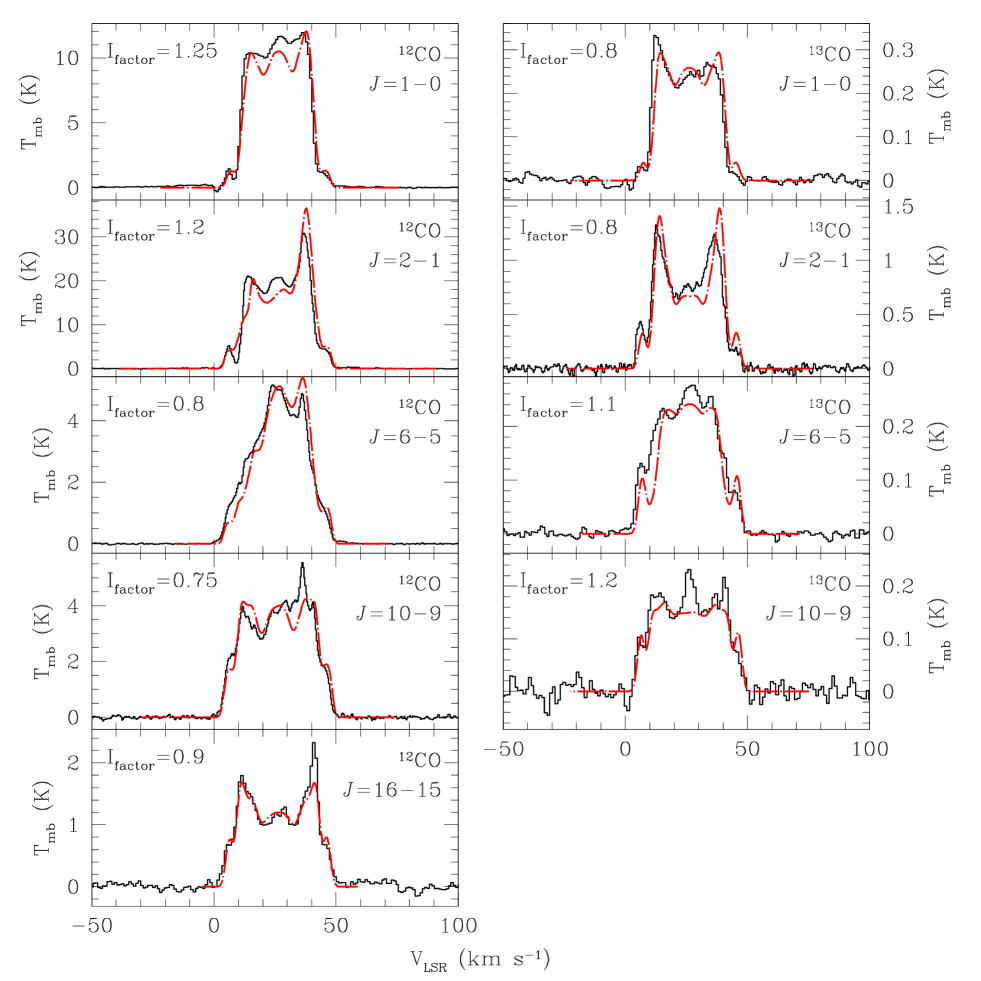
Figure 1: Resulting synthetic spectra (red, dotted-dashed line) and observations (black histogram) for the ¹²CO and ¹³CO transitions detected in NGC 7027. $I_{\mathrm{factor}}$ refers to the intensity factor applied to the model to account for the uncertainties in the model’s radiative transfer solving and in the observations’ calibration.

4.1 Adopted general structure and dynamics

The general structure and dynamics of the model nebula have been deduced from previous imaging (e.g. Nakashima et al., 2010, Cox et al., 2002) and several general properties of our data. Nakashima et al. (2010) find that the molecular gas is located in a hollow axisymmetric shell in expansion, reaching out to 8-10 arcsec from the central star in the equatorial direction. This is slightly more extended than the H₂ shell imaged by Cox et al. (2002), which reaches out to $\sim$5 arcsec in the same direction. The molecular shell is also known to show a low-brightness relatively extended halo (Fong et al., 2006), reaching out to 20-23 arcsec from the central star in the equatorial direction.

Fig. 1 shows the observational profiles of the ¹²CO $J$=1$-$0, 2$-$1, 6$-$5, 10$-$9, 16$-$15, and ¹³CO $J$=1$-$0, 2$-$1, 6$-$5 and 10$-$9 emission (black histogram), along with the synthetic profiles of the best-fit model (red line, see section 4.2). There are a number of features we can deduce from these observational profiles to set the basis for our model. In particular, the blueward intensity fall of the ¹²CO $J$=6$-$5 transition is indicative of strong self-absorption caused by high-opacity and stratification in temperature, which would decrease outwards; also, the peaks of the emission at low and high $J$ occur at different velocities, with absolute radial velocity (with respect to the systemic velocity) increasing with $J$, which in turn indicates simultaneous stratification in velocity and temperature.

We have associated the highest-velocity, low-intensity features visible in our data on both sides of the center of each profile with a pair of unresolved features visible at those velocities in the ¹²CO $J$=2$-$1 maps by Nakashima et al. (2010). They are confined in two small regions along the projection of the nebular main axis on the plane of the sky, at offsets of $\sim$4 arcsec. They appear to lie inside the main envelope of the nebula, closer to the central star. We have interpreted these as a pair of high-velocity blobs ejected by the central star in the polar direction.

Some features and parameters of the model can be deduced exclusively from the conclusions of previous works. Given that the profiles from Herschel/HIFI and the IRAM 30-m radio-telescope contain little information on the morphology of the molecular envelope, we have assumed a basic geometry and size similar to those found by Cox et al. (2002) and Nakashima et al. (2010) for H₂ and CO respectively, consisting of a bipolar 8-shaped shell with a wide waist. We have assumed the inclination to the line of sight and position angle of the main axis of our model to be the same as those found by Nakashima et al. (2010), i.e. $i$=60^∘ and P.A.=155^∘. Summarizing, we have extended the structure described by Cox et al. (2002) taking into account the findings of Nakashima et al. (2010).

The comparison between the position-velocity plots in H₂ (Fig. 4 in Cox et al., 2002) and in ¹²CO $J$=2$-$1 (Fig. 5 in Nakashima et al., 2010), confirms the stratification of the temperature and velocity. The velocity width of the H₂ envelope, which lies closer to the star than the CO envelope, is $\sim$15 km s^-1larger than that of ¹²CO $J$=2$-$1, making it reasonable to assume that the innermost shell of the CO envelope is also the hottest, and that the shells get cooler and more diffuse with increasing distance to the star.

In our modeling, we have adopted a distance of 1 kpc following the results obtained by Zijlstra (2008) from the comparison of the velocity field and apparent expansion at radio wavelengths during a 25-year monitoring period (980$\pm$100 pc).

We consider the aforementioned general considerations and parameters as fixed in our modeling. Additionally, for the density, temperature, and abundance, we used the values found by Cox et al. (2002) in their Fig. 13 as starting points for the model iteration process. Note, however, that our model focus on studying the general physical properties and will necessarily be simple compared with the complex level of details (e.g. holes, clumping, inhomogeneities, etc.) shown by the data in Nakashima et al. (2010) and Cox et al. (2002). The model will therefore focus on reproducing the main features of the observational data, but will not provide an accurate fit of the inhomogeneities and other local details.

4.2 Best-fit model

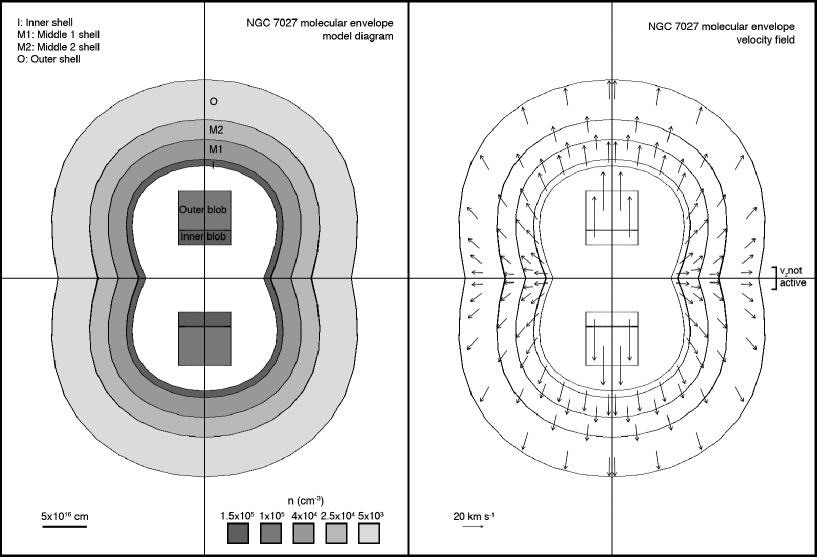
Figure 2: Left: Schematic representation of the model of the molecular envelope of NGC 7027. The shells and blobs are colored according to their densities, in a logarithmic scale. The axes denote the equatorial and polar directions. Right: Velocity field of the model, resulting from the combination of radial and polar components, both pointing outwards from the central star. The polar component is activated for distances to the equator greater than 1.5$\times$10¹⁶ cm (the region where it is not active is indicated). The velocity of the polar blobs is purely along the polar direction.

The model was fit to the data following an iterative trial-and-error procedure. Starting from a set of initial assumptions based on previous works (see previous subsection), we modified each parameter over a large range and solved the radiative transfer equation to obtain a synthetic profile for each of the nine ¹²CO and ¹³CO observational transitions. Each of these synthetic profiles were overlaid on the corresponding observational profiles, and the global quality of the fit assessed by eye as a compromise between the shape of the profile and the intensity at each frequency. When a fair fit was found for all the transitions, we varied the parameters of the model over a smaller range which still provided a fair fit, in order to find the uncertainty of each parameter. This process was repeated several times starting from a different set of parameters. In all cases, the model converged to similar values of every parameter.

A schematic representation of the best-fit model can be seen in Fig. 2, while the associated parameters are shown in tables 2 and 3. Note that due to the vast difference in transition frequencies and origin of the data (ground and space-based), we cannot rule out the presence of relative calibration errors. Therefore, we have included a intensity factor per transition, i.e. the factor to be applied to the intensity of the modeled profile. This factor also accounts for computational errors, and is to be considered as the conservative error of the intensity of our model. In all cases, the intensity of the model profiles were within a 25% of the observed profiles (see the applied intensity factors in Fig. 1). It is noteworthy to point out that the predicted peak intensity of the model at the ¹³CO $J$=16$-$15 transition, 30 mK, is compatible with the non-detection of such line, which peaks at 50$\pm$30 mK, at a resolution in velocity of 4 km s^-1.

In the following we give a detailed description of the different features of the model, i.e the main body of the nebula and the high-velocity polar blobs. These results are essentially compatible with, but more detailed than the preliminary ones provided in Santander-Garcia et al., 2011, whose analysis did not include ¹³CO transitions.

In all cases, we found the best-fitting values of the ¹²CO/¹³CO abundance ratio and micro-turbulence $\delta_{\mathrm{V}}$ to be 50, and 2 km s^-1, respectively. The best-fit for the systemic velocity was $V_{\mathrm{LSR}}$=26.3 km s^-1.

4.2.1 Main body of the nebula

The main body of the nebula consists of four nested, wide waist, 8-shaped shells, arranged in a fashion similar to a Matryoshka or Russian Doll, with each shell in contact with the adjacent ones. Their shape is roughly similar but more extended than the model by Cox et al. (2002) for the H₂ emission. Each of the shells is characterized by a relatively simple set of parameters: equatorial and polar maximum radii, $r_{\mathrm{e}}$ and $r_{\mathrm{p}}$, a thickness $\Delta r$, single values of the abundance $X$(CO), temperature $T$, and density $n$ for the whole shell; and two characteristic velocities, $V_{\mathrm{r}}$ and $V_{\mathrm{z}}$. The total expansion velocity is the combination of these velocities, where $V_{\mathrm{r}}$ is constant, outwards from the central star in the radial direction, and $V_{\mathrm{z}}$ is constant, directed along the polar axis, also outwards from the equator. In all cases, $V_{\mathrm{z}}$ is only triggered for distances to the equator larger than 1.5$\times$10¹⁶ cm. A similar behavior of the velocity is observed in other young PNe or PPNe such as M 1-92 (Bujarrabal et al., 1998), M 2-56 (Castro-Carrizo et al., 2002) and CRL 618 (Sánchez Contreras et al., 2004).

Each shell is tagged by an index according to their location: I, M1, M2, O, after inner, middle 1, middle 2 and outer, respectively. The inner shell I is located just outside the PDR, surrounding the H₂ emission shell model by Cox et al. (2002), and is the main contributor to the features seen in the highest-$J$ spectrum, while the outermost shell O is the coldest, extending to a maximum distance of 2.25$\times$10¹⁷ cm, which projects to 15 arcsec on the plane of the sky. This is slightly larger than the structure visible in $J$=2$-$1 in the maps by Nakashima et al. (2010), but similar in size to the envelope revealed by the $J$=1$-$0 maps by Fong et al. (2006). This discrepancy can be explained by the large extent and smoothness of the envelope, which would make this outermost shell prone to flux-loss (as it would be partially resolved out) in interferometric observations, specially at higher frequencies, as Nakashima et al. (2010) expects for the $J$=2$-$1 emission.

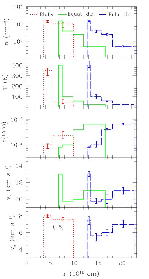
Figure 3: The different parameters of the model of the molecular envelope of NGC 7027 against the distance to the central star, for the equatorial (thick green line) and polar (dotted-dashed blue line) directions, and the polar blobs (dotted red line). The error bars have been drawn at the center of each shell for the blobs and polar direction only (the errors in the equatorial direction are the same as in the polar direction). Note: The velocity (and its error bars) of the polar blobs has been divided by 5 for displaying purposes.

Fig. 3 shows the behavior of the different parameters along the equatorial and polar directions, while the right side of Fig. 2 displays a vector plot of the velocity field. Aside from the highly direction-dependent velocities, and given that the shells are characterized by single values of the parameters, the behavior of $X$, $T$, and $n$ are similar in every direction, as they experiment the same jumps, only at different distances from the central star. The different parameters are essentially compatible with the smooth gradients which would be expected in post-AGB ejecta (see e.g. Justtanont et al., 1994, Goldreich & Scoville, 1976), except for the steep jump between the thin, I shell and the thicker M1 shell. The abundance increases by a factor 1.25 across the I to M1 shell discontinuity, while the density and temperature drop by factors 3.75 and 4 respectively. The velocities $V_{\mathrm{r}}$ and $V_{\mathrm{z}}$ both drop by 25%, a change much more abrupt than the slight, steady increase in velocity from M1 to the outer layers M2 and O.

We take these jumps as clear indications of a shock front traveling outwards through the nebula, in a similar way as the low-velocity shock front found for instance in CRL 618 (e.g. Bujarrabal et al., 2010), in which a double shell is expanding against the nebular halo. The post-shock gas would then naturally be denser, hotter, faster, and less rich in molecules, as a small fraction of those would have been dissociated by the physical conditions at the outer boundary of the PDR and the passing shock front. The presence of this shock implies an increased chance of molecular reactions, which could partly explain the presence of H₂O (see section 4.4). Also, the shock would have strong implications in the shaping of the nebula (Balick & Frank, 2002).

While this relatively simple model does not include a detailed description of the geometry or inhomogeneities/peculiarities of the shells (Nakashima et al., 2010), it is useful to estimate the amount of matter that emits under certain physical conditions. Taking into account the volume and density of each shell, we can derive the molecular mass distribution. Adding up every shell, the total molecular mass we estimate for the main molecular envelope of NGC 7027 is 1.15 M_⊙, which agrees well with previous estimates of 1.2 M_⊙ by Fong et al., 2001.

The kinematic age of the inner, presumably shocked shell is $\sim$1700-2000 years (computed at the equator and poles respectively). The rest of the envelope ranges from $\sim$2800-3000 years for the M1 shell to $\sim$4300-4700 years for the O one. This time-difference is not model-dependent, as it arises directly from the observations, and is also visible in the data from previous works (e.g. Nakashima et al., 2010; Fong et al., 2006). This suggests that the expansion pattern of the molecular envelope is not compatible with a single-event, pure ballistic expansion or Hubble-like flow, and was instead ejected during a time-interval larger than 1000 years. It is interesting to note that, in this case, the value of $n\times r^{2}$ (density corrected for the dilution into the medium) decreases with the kinetic age of the outflow, while the expansion velocity increases. This is expected if along the AGB evolution the stars approaches increases in its mass loss. Another possibility, though, would be that the nebula has been affected by a series of front shocks, resulting in different apparent kinematic ages.

Table 2: Best-fit model parameters for the main molecular envelope of NGC 7027. The sizes correspond to a distance to the nebula of 1 kpc. The uncertainty range is included for every parameter except the sizes of the shells, which depend on the corresponding uncertainties on the shell thicknesses.

Shell	$r_{\mathrm{polar}}^{\dagger}$	$r_{\mathrm{equatorial}}^{\dagger}$	$\Delta r^{\star}$	$V_{\mathrm{r}}^{\ddagger}$	$V_{\mathrm{z}}^{\mathrm{*}}$	$X{\mathrm{(}^{12}\mathrm{CO)}}$	$n$	$T$
	(1016 cm)	(1016 cm)	(1016 cm)	(km s-1)	(km s-1)		(cm-3)	(K)
I: Inner shell	13.5	7.5	0.75${}^{+0.15}_{-0.15}$	13.0${}^{+0.3}_{-0.3}$	7.5${}^{+0.4}_{-0.5}$	8${}^{+0.3}_{-0.4}\times$10-5	1.5${}^{+0.05}_{-0.1}\times$105	400${}^{+40}_{-20}$
M1: Middle 1 shell	15.75	9.75	2.25${}^{+0.25}_{-0.35}$	9.75${}^{+0.35}_{-0.25}$	5.6${}^{+0.3}_{-0.6}$	1${}^{+0.4}_{-0.2}\times$10-4	4.0${}^{+0.8}_{-0.8}\times$104	100${}^{+20}_{-20}$
M2: Middle 2 shell	18.0	12.0	2.25${}^{+0.35}_{-0.35}$	10.0${}^{+0.6}_{-0.5}$	6.0${}^{+0.4}_{-0.4}$	4${}^{+0.4}_{-0.4}\times$10-4	2.5${}^{+0.25}_{-0.25}\times$104	60${}^{+6}_{-6}$
O: Outer shell	22.5	16.5	4.5${}^{+0.6}_{-0.6}$	11.0${}^{+0.4}_{-0.4}$	7.0${}^{+0.5}_{-0.4}$	6.7${}^{+0.5}_{-0.6}\times$10-4	5.0${}^{+0.5}_{-0.4}\times$103	25${}^{+3}_{-2}$

Notes: The $X$(¹³CO) abundances are 50 times lower than their $X$(¹²CO) counterparts.
^†Distance from the star which traces the shell’s outer edge, both at the pole and equator.
^⋆ Thickness of the shell.
^‡ Expansion velocity radially outwards from the central star.
^∗ Additional velocity component along main axis. Activated for distances to the equator greater than 1.5$\times$10¹⁶ cm.

4.2.2 High-velocity polar blobs

Unfortunately, data from previous works lack enough spatial resolution to resolve the geometry of the polar blobs. Therefore, we chose to model them in a simple way as two small cylinders being ejected from the central star along the nebular main axis. The reason for choosing cylinders and not other geometrical shapes (e.g. spheres) is for mere convenience: each cylinder is easily split in two sections with different physical conditions. Each section is characterized by a height, a radius, a distance from the equatorial plane to its center, and single values of $T$, $X$ and $n$. The velocity of each section is constant and its direction is axial (i.e. parallel to the main axis of the nebula). The best-fit parameters of the modeling are shown in Table 3 and Fig. 3 (dotted red line).

The aft section, located closer to the central star, is thinner, hotter and denser than the fore one, which center is 7.65$\times$10¹⁶ cm offset from the star, so that its projection unto the plane of the sky coincides with the small, high-velocity region visible in the ¹²CO $J$=2$-$1 maps by Nakashima et al. (2010) at offsets of $\sim$4 arcsec. However, it is noteworthy to remark that, specially in this case, we do not have enough observational data to further constrain the blobs geometry, since there is no indication whatsoever of the spatial origin of the high-velocity emission at higher $J$. Therefore, the location of the hotter and denser cylinder section in the aft (and not in the fore as a bow-shock) is purely arbitrary, and have no further consequences in the modeling. Given its slightly larger velocity, and its increased density and temperature, it would be tempting to relate these jumps to the action of shocks, as a result of a front shock travelling through the nebula and catching up on the blobs, or a bow-shock in the fore section as the blobs expand against the PDR and molecular envelope. Unfortunately, the data at hand prevents further interpretation. We can only conclude on the existence of at least two components with different physical conditions. Further observations should provide independent insight on the properties of these blobs.

From our model we estimate a total mass of the blobs of 0.1 M_⊙, under the aforementioned uncertainties. Therefore the total mass of the nebula, taking into account all the components, agrees well with previous determinations.

Finally, at the adopted distance, the kinematical age of the blobs is in the range 360-630 yrs. Given that this value range is not model-dependent, this implies that the blobs are much younger than the rest of the molecular envelope, including the shocked, inner shell, whose kinematical age is a factor 3-4 larger. This suggests that the blobs were ejected approximately during the same epoch as (or immediately after than) the inner H ii nebula, which strongly emits at radio wavelengths (600 yrs, see Masson, 1989). An alternative explanation, however, would be that the blobs are in fact older, but have been progressively accelerated by ram pressure by the faster-expanding inner H ii nebula.

Table 3: Best-fit model parameters for the high-velocity polar blobs of NGC 7027. The sizes correspond to a distance to the nebula of 1 kpc. The uncertainty range is included for every parameter except the distance of the structure to the central star, which is assumed a priori based on existing maps.

Blob section	$d_{\mathrm{off}}^{\dagger}$	$r^{\ddagger}$	$h^{\star}$	$V^{\mathrm{*}}$	$X{\mathrm{(}^{12}\mathrm{CO)}}$	$n$	$T$
	(1016 cm)	(1016 cm)	(1016 cm)	(km s-1)		(cm-3)	(K)
Inner	4.5	3.0${}^{+0.2}_{-0.4}$	1.65${}^{+0.15}_{-0.45}$	40.0${}^{+1}_{-1}$	1${}^{+0.1}_{-0.3}\times$10-4	1.5${}^{+0.1}_{-0.25}\times$105	350${}^{+25}_{-50}$
Outer	7.65	3.0${}^{+0.3}_{-0.6}$	4.5${}^{+0.3}_{-0.4}$	38.0${}^{+1}_{-1}$	2.3${}^{+1.0}_{-0.5}\times$10-4	1${}^{+0.2}_{-0.4}\times$105	50${}^{+25}_{-15}$

Notes: The $X$(¹³CO) abundances are 50 times lower than their $X$(¹²CO) counterparts.
^†Distance from the star to the center of mass of the given cylindrical section.
^⋆ Radius of the cylinder.
^‡ Height of the cylindrical section.
^∗ Velocity of the cylindrical section along the main axis of the nebula.

4.3 Uncertainty of the model parameters

Given the high-degree of interaction between the different model parameters, it is difficult to assess their range of uncertainty. Contrary to standard spatio-kinematical modeling, where the effect of changing a parameter is easily followed (e.g. a velocity near the lower limit of the uncertainty range corresponds to an age-distance parameter close to the upper limit, see Santander-García et al. 2004 as an example), the effects of almost any parameter change in a radiative-transfer spatio-kinematical model are non-trivial to predict.

Tables 2 and 3 show conservative estimations of the uncertainty range of every model parameter. The range for each parameter has been obtained by fixing every other parameter of the model and allowing the given parameter to change until it no longer provided a fair fit to the data (i.e. until the intensity factors to be applied to the model profiles no longer lied within the 25% of the observed intensities, except in the case of the velocities, where the fairness of the fit was assessed by eye). Most of the uncertainty ranges of the model lie within a 10% of the best-fit values, except the temperature and density of the M1 shell, both of which reach a 20%; its abundance, which reaches a 40%; and the temperature, abundance and temperature of the blobs, some of which reach an uncertainty of $\sim$40% of its best-fit value.

These uncertainty ranges, however, should be considered as a simplistic approach to the real errors. In fact, if multiple parameters were allowed to change, the uncertainty ranges would be somewhat larger: for example, an increase in temperature can be partially acommodated by a decrease in density, and viceversa. Since, given the parameter interdependence, it would be impossible to compute the uncertainty ranges with as many degrees of freedom as parameters in the model, we hereby provide the following representative example. The temperature of the inner shell can be increased to 520 K if the density drops to 1.3$\times$10⁵ cm^-3, or the temperature decreased to 360 K and the density increased to 1.6$\times$10⁵ cm^-3, and still provide a fair-fit to the data. This represents an increase in uncertainty for the temperature from 10% to 30%, and from 10% to 13% for the density.

4.4 Other molecules

The electronic level population is significantly more complicated for molecules more complex than CO, making the computation of their absorption and emission coefficients a daunting task. Hence, a detailed analysis including radiative-transfer solving of other molecular species such as H₂O in NGC 7027 has been kept out of the focus of this study. However, it is interesting to do a qualitative analysis of the data in order to lay the foundations of future work.

H₂O: The presence of the H₂O 1${}_{1,0}-$1_0,1 and 1${}_{1,1}-$0_0,0 transitions in the spectrum of NGC 7027 is striking, given that NGC 7027 is a C-rich PNe. In fact, to our knowledge, aside from this case, H₂O has been detected in only two C-rich PNe, CRL 618 (Bujarrabal et al. 2012) and CRL 2688 (Wesson et al., 2010).

The H₂O profiles (see Fig. 5 in Bujarrabal et al., 2012) somewhat resemble the high-excitation profiles of ¹²CO (especially that of $J$=16$-$15). The relative weakness of these profiles, in comparison with those of CO at similar frequencies (i.e. similar beam size), reveals that the nebula is optically thin at those transitions. The comparison of the H₂O and CO profiles, in view of our model of the molecular envelope, seems to suggest that most of the water lies within the inner, faster shell, or even closer to the PDR, since the velocity separation between two peaks of the H₂O 1${}_{1,0}-$1_0,1 and 1${}_{1,1}-$0_0,0 profiles are $\sim$30.8 and $\sim$31.9 km s^-1respectively. These values are slightly larger than the peak separation in every CO profile, including the highest $J-$line observed, 16$-$15, which is $\sim$29.7 km s^-1.

It is known that water is already abundant in the circumstellar envelopes around AGB stars (Neufeld et al., 2011). However, the fact that water seems to be particularly abundant in the inner shells of NGC 7027 suggests an ongoing process of water production in this source, either due to the passage of a shock front or photo-induced chemistry. We consider photo-induction by the UV radiation from the central star to be the more likely cause, since while the shock is relatively weak (see section 4.2.1), most of the water would lie close to the extremely hot (T${}_{\mathrm{eff}}\sim$200,000 K) star. This explanation is compatible with the findings of Bujarrabal et al. (2012) in CRL 618 and CRL 2688. CRL 618 shows a narrower water profile than those of CO, indicative of it being concentrated closer to the hot (T${}_{\mathrm{eff}}\sim$30,000 K) star, while there is no significant increase of the abundance in the shocked region. On the contrary, CRL 2688 shows a shocked region but no water, while the central star is too cool (T${}_{\mathrm{eff}}\sim$7,000 K) to emit a significant amount of UV radiation.

C¹⁸O: The emission in C¹⁸O is weak and optically thin (see Fig. 4 in Bujarrabal et al., 2012). In view of our model, it appears to come primarily from the regions close to the equatorial plane. This could indicate that this ring is denser than the rest of the bipolar shell, or show matter condensations, in a very clumpy general structure.

OH: The OH profile is very weak (see Fig. 5 in Bujarrabal et al., 2012). Although OH is usually associated with the region where H₂O is dissociated (e.g. Goldreich & Scoville, 1976), the shape of the profile is very different than those of water. In light of the present data, any further attempt at interpreting this profile is unclear.

5 Conclusions

The main results of this work are summarized in what follows:

1. We have developed a software code, shapemol, which, used along with SHAPE (Steffen et al., 2011), implements spatio-kinematical modeling with accurate calculations of non-LTE line excitations and radiative transfer in molecular species. A more detailed description of shapemol will be given by Santander-García et al. in a forthcoming paper.

2. Based on observations of a series of low and high-excitation ¹²CO and ¹³CO transitions by Herschel/HIFI and the IRAM 30-m radiotelescope, we have used shapemol and SHAPE to build a model of the molecular envelope of the young PNe NGC 7027. The geometry of the model is based in existing maps and data from CO and H₂ (see section 4.1). This model consists of four nested mildly-bipolar shells and a pair of high-velocity polar blobs (see Fig. 2). Each shell is charaterised by single values of the abundance, temperature, density and velocity. Since the profiles contain little information on the spatial structure of NGC 7027, the geometry of our model should be considered as a rough approximation.

3. The temperature of the shells ranges from 400 K for the innermost and 25 K for the outermost ones. The density also drops down from 1.5$\times$10⁵ cm^-3 in the innermost shell to 5$\times$10³ cm^-3 in the outermost one, while the ¹²CO relative abundance increases from 8$\times$10^-5 to 6.7$\times$10^-4. The ¹²CO/¹³CO abundance ratio is 50, while the microturbulence, $\delta_{\mathrm{V}}$, is 2 km s^-1.

4. The expansion pattern of the shells is not compatible with a Hubble-like flow. Instead, the 3-D velocity field of each shell is a combination of a constant, purely radial motion plus an additional constant component along the main axis of the nebula. The latter is only activated for distances to the equator larger than 1.5$\times$10¹⁶ cm (at the adopted distance of 1 kpc to the nebula). The velocity of each consecutive outer shell is slightly larger than the preceding inner one, with the following exception:

5. The innermost shell is thinner than the rest, and is characterized by anomalous physical conditions: its expansion velocity is 33% higher than that in the adjacent intermediate shell. The abundance also increases a factor 1.25 across the inner-to-intermediate shell discontinuity, while the density and temperature drop by factors of 3.75 and 4 respectively. We interpret these jumps as indicative of a passing shock front. This shock could have important implications in the shaping of the nebula.

6. Each of the two opposing polar blobs is assumed to be a small cylinder split in two sections with very different physical conditions. One of them is hot (350 K) and dense (1.5$\times$10⁵ cm^-3), has a ¹²CO abundance of 1$\times$10^-4 and a slightly larger velocity (40 km s^-1) than the other one (38 km s^-1), which is much cooler (50 K), tenuous (1$\times$10⁵ cm^-3) and shows a larger ¹²CO abundance (2.3$\times$10^-4). The shape of the blobs, as well as the relative position of the cylinders (whether the hotter and denser is located at the fore or the aft of the blob) in the model is an arbitrary choice, given that the emission from the blobs is unresolved in the maps available in the literature and cannot therefore be determined from existing data. Whether the blobs are affected by the same shock front as the inner shell or they form bow shocks in their advance against the PDR and molecular envelope is therefore unclear.

7. The computed molecular mass of the main nebula is 1.15 M_⊙, while the mass of the blobs is 0.1 M_⊙, adding to a total molecular mass for NGC 7027 of roughly 1.3 M_⊙. This figure is compatible with those derived by previous works.

8. The presence of H₂O in the spectrum of NGC 7027, a C-rich nebula, is striking. From the profiles of the two detected transitions we conclude that the water is formed in a region close to the shocked inner shell, if not even slightly closer to the extremely hot central star. We cannot rule out the possibility of shocks as the leading mechanism in the formation of water. However, given the proximity to the extremely hot central star, we consider more likely that the formation is mainly photo-induced by UV radiation from the star.