Quantum gates and multipartite entanglement resonances realized by non-uniform cavity motion

Abstract

We demonstrate the presence of genuine multipartite entanglement between the modes of quantum fields in non-uniformly moving cavities. The transformations generated by the cavity motion can be considered as multipartite quantum gates. We present two setups for which multi-mode entanglement can be generated for bosons and fermions. As a highlight we show that the genuine bosonic multipartite correlations can be resonantly enhanced. Our results provide fundamental insights into the structure of Bogoliubov transformations and suggest strong links between quantum information, quantum fields in curved spacetimes and gravitational analogues by way of the equivalence principle.

I Introduction

During the past decade research in the area of relativistic quantum information has addressed questions concerning the inherently relativistic aspects of quantum phenomena, unveiling the close connections between effects in quantum field theories and quantum information theory.

In this context several models to store and access bipartite quantum correlations in relativistic settings have been proposed, including Unruh-DeWitt type detector models HuLinLouko2012 , free field modes BruschiLoukoMartin-MartinezDraganFuentes2010 ; DownesRalphWalk2012 ; DraganDoukasMartin-MartinezBruschi2012 and cavity modes (see Refs. DownesFuentesRalph2011 ; BruschiFuentesLouko2012 ; FriisLeeBruschiLouko2012 ; FriisBruschiLoukoFuentes2012 ; FriisFuentes2012 ; BruschiDraganLeeFuentesLouko2012 for details and Ref. AlsingFuentes2012 for a recent review).

In these situations bipartite entanglement was extensively studied but, save for a few exceptions AlsingFuentes-SchullerMannTessier2006 ; AdessoFuentes-SchullerEricsson2007 ; AdessoFuentes-Schuller2009 ; HuberFriisGabrielSpenglerHiesmayr2011 ; SmithMann2012 , the role of genuine multipartite correlations in these studies was marginal. However, multipartite correlations are expected to feature in relativistic scenarios, e.g., in the transformation of Minkowski modes to Rindler modes BruschiLoukoMartin-MartinezDraganFuentes2010 . Moreover, they become ever more prominent as the size and complexity of the systems in question increase. In these scenarios the classification of genuine multipartite entanglement will allow for a more detailed characterization of relativistic effects and may be used for high-sensitivity tests that indicate the “quantumness” of relativistic phenomena. In fact, the identification of quantum correlations can be a keystone to the experimental verification of effects in quantum field theory, such as the Hawking effect in analog fluid systems, see Ref. RecatiPavloffCarusotto2009 .

Here we want to focus on the generation of genuine multipartite entanglement by the non-uniform motion of cavities that contain relativistic quantum fields. We employ the techniques developed in Refs. BruschiFuentesLouko2012 ; FriisLeeBruschiLouko2012 , for bosonic and fermionic fields respectively, where the moving cavities follow worldtubes that are composed of segments of inertial motion and uniform acceleration. In this framework we ask the questions: Can the Bogoliubov transformations that are induced by the non-uniform motion generate genuine multipartite, quantum correlations? If this is the case, can we quantify and/or classify the arising entanglement?

We present two scenarios for which we can indeed create, and partially classify, such correlations, thereby realizing quantum gates by motion. First, in Sec. II, we consider three individual cavities, labelled Alice, Rob and Charlie, that share pairwise bipartite entanglement in their initially common rest-frame, before Rob’s cavity undergoes non-uniform motion, see Fig. 1. In the second scenario we consider Rob’s cavity on its own in Sec. III. In these scenarios the significantly different advantages of bosonic and fermionic systems become apparent.

In the bosonic case the transformations induced by the cavity motion generate multi-mode entangling quantum gates. Moreover, we show that the genuine multipartite character of the bosonic entanglement can be enhanced resonantly by appropriate timing of the cavity’s trajectory segments. The qubit structure of the fermionic systems, on the other hand, allows for a clear classification of the arising multipartite correlations. The cavity motion effectively acts as a multipartite quantum gate producing Dicke states and $W$ states. We present explicit pure state decompositions for these classifications in Secs. II.2 and III.2, respectively.

The calculation of the Bogoliubov transformations for the non-uniform cavity motion are performed perturbatively in terms of a parameter $h$ that physically represents the product of the (rest-frame) cavity width $\delta$ and the acceleration at the centre of the cavity. Using the Bogoliubov coefficients obtained in this way we can perform all other computations analytically. For simplicity we restrict our considerations to $(1+1)$-dimensional Minkowski spacetime where the metric tensor $\eta_{\mu\nu}$ has the signature $(-,+)$. The setup can be naturally extended to accommodate additional spatial dimensions that enter into the effective mass of the field via the corresponding transverse momenta BruschiFuentesLouko2012 . We use units where Planck’s constant and the speed of light are dimensionless, i.e., $\hbar=c=1$. By $O(x)$ we denote a quantity for which $O(x)/x$ remains bounded as $x$ goes to zero. We use an asterisk and a dagger to denote complex and Hermitian conjugation respectively.

II Multi-cavity entanglement

As the first scenario we consider three cavities, Alice, Rob and Charlie. Each cavity represents an individual spacetime in which a relativistic quantum field is confined by appropriate boundary conditions. We can assume without loss of generality that all three cavities are manufactured in the same way and that they are initially (in the “in-region”) at rest with respect to each other. At $t=0$ Rob’s cavity starts to accelerate linearly and uniformly. We assume that the worldtube of Rob’s cavity consists of periods of inertial motion and uniform acceleration such that the cavity remains rigid throughout the journey, i.e., the cavity length $\delta>0$, as measured by the co-moving observer, is constant. For the perturbative treatment we further assume that the accelerations in all individual segments are small with respect to the inverse cavity length $1/\delta$. Fig. 1 shows the spacetime diagram of this setup for a sample travel scenario.

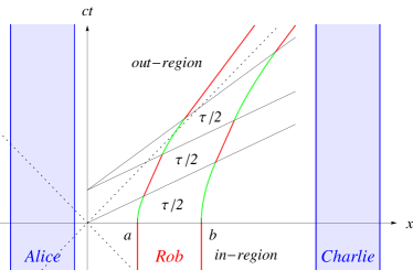
Figure 1: Space-time diagram of the multi-cavity setup: While Alice’s and Charlie’s cavities remain at rest Rob’s cavity undergoes non-uniform motion. Rob’s cavity of width $\delta=(b-a)$ follows a worldtube that consists of alternating segments of inertial motion (red) and uniform acceleration (green). The individual segments in this example travel scenario are of equal duration $\tau/2$ and equal acceleration $h/\delta$ as measured at the centre of Rob’s cavity. The dashed lines indicate the light cone at $(t,x)=(0,0)$.

II.1 Scalar fields

Let us consider a real, scalar field $\phi$ of mass $m\geq 0$ in Rob’s initially inertial cavity in the “in-region”. The field satisfies the Klein-Gordon equation $(-\Box+m^{2})\phi=0$, where $\Box$ is the scalar D’Alambertian. We follow the procedure laid out in Ref. BruschiFuentesLouko2012 and represent the confinement to the cavity by imposing the Dirichlet boundary conditions $\phi(t<0,a)=\phi(t<0,b)=0$. We thus obtain a discrete spectrum of mode functions $\phi_{n}$ in the in-region, where the field can be decomposed as

$$\phi =\sum\limits_{n}\,\Bigl{(}\,\phi_{n}\,a_{n}\,+\,\phi_{n}^{*}\,a_{n}^{\dagger}\,\Bigr{)}\,.$$ (1)

The annihilation and creation operators, $a_{n}$ and $a_{n}^{\dagger}$, satisfy the usual commutation relations $\left[a_{n},a_{m}^{\dagger}\right]=\delta_{nm}$. The vacuum state of the corresponding Fock space is annihilated by all $a_{n}$’s, i.e., $a_{n}\left|\,0\,\right\rangle=0$.

Before we construct our initial state let us briefly recall the characteristics of genuine multipartite entanglement. Any pure quantum state that can be written as a tensor product with respect to any bipartition is called bi-separable. Generalizing this notion to mixed states, any mixed quantum state is called bi-separable if it admits at least one decomposition into a convex sum of pure, bi-separable states. Conversely, all states that are not bi-separable are called genuinely multipartite entangled. See, e.g., Refs. GuehneToth2009 ; GabrielHiesmayrHuber2010 for more details.

We now proceed by constructing an initial state that contains no such genuine multipartite entanglement. We select two of Rob’s modes, $k$ and $k^{\prime}$, and entangle them with modes $A$ and $C$ in Alice’s and Charlie’s cavities respectively. This could be achieved by a scheme similar to that presented in Ref. BrownePlenio2003 . The initial, bi-separable state of the four modes $A,k,k^{\prime}$ and $C$ we denote by

$$\rho^{\,\pm}_{A\!RC} =\left|\right.\!\Phi^{\pm}\!\left.\right\rangle\left\langle\right.\!\Phi^{\pm}\!\left.\right|$$ (2)

with $\left|\right.\!\Phi^{\pm}\!\left.\right\rangle=\left|\right.\!\phi^{\pm}\!\left.\right\rangle_{Ak}\left|\right.\!\phi^{\pm}\!\left.\right\rangle_{k^{\prime}C}$, where the bipartite entangled states are given by

$$\left|\right.\!\phi^{\pm}\!\left.\right\rangle_{Ak} =\tfrac{1}{\sqrt{2}}\,\bigl{(}\,\,\left|\,0\,\right\rangle\,\pm\,\left|\,1_{A}\,\right\rangle\,\left|\,1_{k}\,\right\rangle\,\bigr{)}\,,$$ (3a)

$$\left|\right.\!\phi^{\pm}\!\left.\right\rangle_{k^{\prime}C} =\tfrac{1}{\sqrt{2}}\,\bigl{(}\,\,\left|\,0\,\right\rangle\,\pm\,\left|\,1_{k^{\prime}}\,\right\rangle\,\left|\,1_{C}\,\right\rangle\,\bigr{)}\,.$$ (3b)

At $t=0$ we start to accelerate Rob’s cavity uniformly and linearly and we let it follow a worldtube that consists of segments of inertial motion and uniform acceleration. An example trajectory is shown in Fig. 1. After an arbitrary number of such trajectory segments we assume without loss of generality that the cavity remains inertial in the “out-region”. The mode functions $\tilde{\phi}_{m}$ and their corresponding annihilation and creation operators $\tilde{a}_{m}$ and $\tilde{a}^{\dagger}_{m}$ in the out-region are related to their in-region counterparts by a Bogoliubov transformation with coefficients $\alpha_{mn}$ and $\beta_{mn}$, i.e.,

$$\tilde{\phi}_{m} =\sum\limits_{n}\bigl{(}\alpha_{mn}\phi_{n}+\beta_{mn}\phi_{n}^{*}\bigr{)}$$ (4)

and

$$\tilde{a}_{m} =\sum\limits_{n}\bigl{(}\alpha^{*}_{mn}a_{n}-\beta^{*}_{mn}a^{\dagger}_{n}\bigr{)}.$$ (5)

In the case where the length $\delta=(b-a)$ of the rigid cavity is fixed and the individual accelerations of the cavity at any point of the trajectory are small compared to $1/\delta$ the Bogoliubov coefficients can be computed analytically as a Maclaurin expansion, i.e.,

$$\alpha_{mn} =\alpha^{{}_{(0)}}_{mn}+\alpha^{{}_{(1)}}_{mn}+O(h^{2})\,,$$ (6a)

$$\beta_{mn} =\beta^{{}_{(1)}}_{mn}+\beta^{{}_{(2)}}_{mn}+O(h^{3})\,,$$ (6b)

with $\alpha^{{}_{(0)}}_{mn}=\delta_{mn}G_{m}$ (no summation), see Ref. BruschiFuentesLouko2012 . The $G_{m}$ are phase factors satisfying $|G_{m}|^{2}=1$ that are picked up by the modes during the free time evolution in each segment of the cavity motion. The superscripts ${}^{{}_{(n)}}$ in Eq. (6) indicate the power of the expansion parameters $h_{i}$, which represent the products of the cavity width and the acceleration at the center of the cavity in the $i$-th trajectory segment. For ease of notation we will suppress the subscript $i$ in the remaining discussion.

The Bogoliubov coefficients for any trajectory that is composed of segments of inertial motion and uniform acceleration can be constructed from the coefficients for a single switch from inertial motion to constant acceleration, i.e., coefficients relating Minkowski modes $\phi_{n}$ and Rindler modes $\tilde{\phi}_{n}$, along with phases $G_{n}$ that are picked up by the modes in each segment. A detailed derivation of these coefficients for massless and massive scalar fields as well the construction of generic trajectories can be found in Refs. BruschiFuentesLouko2012 ; BruschiDraganLeeFuentesLouko2012 .

Using well-known standard procedures (see, e.g., Refs. BruschiFuentesLouko2012 or FriisBruschiLoukoFuentes2012 ) the Fock states $\left|\right.\!n_{k}\!\left.\right\rangle$ and $\left|\right.\!n_{k^{\prime}}\!\left.\right\rangle$ of Rob’s cavity in the initial state $\rho^{\,\pm}_{A\!RC}$ can be transformed to the out-region basis $\left|\right.\!\tilde{n}_{i}\!\left.\right\rangle$ to obtain the transformed density matrix $\tilde{\rho}^{\,\pm}_{A\!RC}$. The transformations between the relevant in-region and out-region Fock states up to first order in the perturbative expansion are given by (see Ref. FriisBruschiLoukoFuentes2012 )

$$\left|\right.0\left.\right\rangle\ =\,\left|\right.\tilde{0}\left.\right\rangle\,-\,\tfrac{1}{2}\sum\limits_{p,q}G_{q}^{\,*}\beta_{pq}^{{}_{(1)}\raisebox{-1.7pt}{\scriptsize{$*$}}}\,\tilde{a}^{\dagger}_{p}\tilde{a}^{\dagger}_{q}\,\left|\right.\tilde{0}\left.\right\rangle\,+\,O(h^{2})\,,$$ (7a)

$$\left|\right.1_{k}\left.\right\rangle =\,G_{k}^{\,*}\,\left|\right.\!\tilde{1}_{k}\!\left.\right\rangle\,+\,\sum\limits_{m\neq k}\alpha_{mk}^{{}_{(1)}\raisebox{-1.7pt}{\scriptsize{$*$}}}\,\left|\right.\!\tilde{1}_{m}\!\left.\right\rangle$$ (7b)

$$\,-\,\tfrac{1}{2}G_{k}^{\,*}\sum\limits_{p,q}G_{q}^{\,*}\beta_{pq}^{{}_{(1)}\raisebox{-1.7pt}{\scriptsize{$*$}}}\,\tilde{a}^{\dagger}_{p}\tilde{a}^{\dagger}_{q}\,\left|\right.\!\tilde{1}_{k}\!\left.\right\rangle\,+\,O(h^{2})\,,$$

$$\left|\right.\!1_{k}\!\left.\right\rangle\left|\right.\!1_{k^{\prime}}\!\left.\right\rangle =\,G_{k}^{\,*}\beta_{kk^{\prime}}^{{}_{(1)}}\,\left|\right.\tilde{0}\left.\right\rangle\,+\,G_{k}^{\,*}\!\sum\limits_{m\neq k^{\prime}}\alpha_{mk^{\prime}}^{{}_{(1)}\raisebox{-1.7pt}{\scriptsize{$*$}}}\,\tilde{a}_{m}^{\dagger}\,\left|\right.\!\tilde{1}_{k}\!\left.\right\rangle$$

$$\,+\,G_{k}^{\,*}G_{k^{\prime}}^{\,*}\,\left|\right.\!\tilde{1}_{k}\!\left.\right\rangle\left|\right.\!\tilde{1}_{k^{\prime}}\!\left.\right\rangle\,+\,G_{k^{\prime}}^{\,*}\!\sum\limits_{m\neq k}\alpha_{mk}^{{}_{(1)}\raisebox{-1.7pt}{\scriptsize{$*$}}}\,\tilde{a}_{m}^{\dagger}\,\left|\right.\!\tilde{1}_{k^{\prime}}\!\left.\right\rangle$$

$$\,-\,\tfrac{1}{2}G_{k}^{\,*}G_{k^{\prime}}^{\,*}\!\sum\limits_{p,q}G_{q}^{\,*}\beta_{pq}^{{}_{(1)}\raisebox{-1.7pt}{\scriptsize{$*$}}}\,\tilde{a}_{p}^{\dagger}\tilde{a}_{q}^{\dagger}\,\left|\right.\!\tilde{1}_{k}\!\left.\right\rangle\left|\right.\!\tilde{1}_{k^{\prime}}\!\left.\right\rangle\,,$$ (7c)

and the transformation of $\left|\right.\!1_{k^{\prime}}\!\left.\right\rangle$ can be obtained from (7b) by replacing $k$ with $k^{\prime}$.

Subsequently, we trace over all of Rob’s out-region modes except $k$ and $k^{\prime}$, gaining the reduced density operator $\tilde{\rho}^{\,\pm}_{Akk^{\prime}C}$ of the four bosonic modes $A,k,k^{\prime}$ and $C$. Keeping terms up to first order in $h$ we find that $\tilde{\rho}^{\,\pm}_{Akk^{\prime}C}$ is effectively a state of two qubits, the modes $A$ and $C$, and two qutrits, the modes $k$ and $k^{\prime}$. In other words, to first order in $h$ the modes $A$ and $C$ are not further populated by the Bogoliubov transformation and their respective Hilbert spaces can be truncated to single-qubit, i.e., two-dimensional, Hilbert spaces with basis vectors $\left|\right.\tilde{0}_{k}\!\left.\right\rangle,\left|\right.\!\tilde{1}_{k}\!\left.\right\rangle$ and $\left|\right.\tilde{0}_{k^{\prime}}\!\left.\right\rangle,\left|\right.\!\tilde{1}_{k^{\prime}}\!\left.\right\rangle$ respectively. For the modes $k$ and $k^{\prime}$, on the other hand, the states $\left|\right.\!\tilde{2}_{k}\!\left.\right\rangle$ and $\left|\right.\!\tilde{2}_{k^{\prime}}\!\left.\right\rangle$ are populated by the cavity motion. This means the description of these modes involves at least three basis vectors each, i.e., the modes effectively become qutrits.

For such states a general quantification of genuine multipartite entanglement proves to be cumbersome, as there is no general classification scheme for multipartite systems beyond qubits. However, we can construct an inequality that acts as a witness for genuine multipartite entanglement by comparing diagonal- and off-diagonal elements of $\tilde{\rho}^{\,\pm}_{Akk^{\prime}C}$. The construction of such a witness is straightforward: We exploit permutation symmetries of bi-separable pure states to construct a convex function of density matrix elements that satisfies a simple inequality. The convexity of this function ensures that bi-separable mixed states satisfy the inequality. Consequently, its violation detects genuine multipartite entanglement in mixed states, see Refs. GabrielHiesmayrHuber2010 ; MaChenChenSpenglerGabrielHuber2011 ; WuKampermannBruszKloecklHuber2012 . Since the diagonal elements that are newly generated by the Bogoliubov transformation are at least $O(h^{2})$ the witness inequality, whose complete form is given by Eq. (31) of the appendix, takes the simple form

$$2\,\left|\left\langle\right.\!1_{C}\!\left.\right|\left\langle\right.\!\tilde{2}_{k^{\prime}}\!\left.\right|\left\langle\right.\!\tilde{2}_{k}\!\left.\right|\left\langle\right.\!1_{A}\!\left.\right|\,\tilde{\rho}^{\,\pm}_{Akk^{\prime}C}\,\left|\right.\tilde{0}\left.\right\rangle\right|\,-\,O(h^{2})\, \leq\,0\,.$$ (8)

Evaluating the matrix element we can recast (8) as

$$\tfrac{1}{2}|\beta^{{}_{(1)}}_{kk^{\prime}}|\,-\,O(h^{2}) \leq\,0\,.$$ (9)

Within the perturbative regime this inequality is violated, i.e., genuine multipartite entanglement is detected, whenever $\beta^{{}_{(1)}}_{kk^{\prime}}\neq 0$. This is the case for all mode pairs of opposite parity, i.e., if $(k-k^{\prime})$ is odd. If the modes $k$ and $k^{\prime}$ have the same parity the first order coefficients relating these two modes vanish identically and statements about the violation of inequality (8) can only be made for given mode numbers and the answers will depend on the particular cavity motion. We will therefore employ (8) to first order in $h$ as witness for the detection of genuine multipartite entanglement.

In fact, (9) is not only a witness, but also a lower bound to a measure of genuine multipartite entanglement, the generalization of the concurrence to multipartite entanglement. This type of concurrence is based on the linear entropy, which, in turn, is chosen in this context only to write the witness in a compact form. However, any lower bound on a measure based on the linear entropy supplies a lower bound to that same measure based on the physically more intuitive Rényi-2 entropy WuKampermannBruszKloecklHuber2012 . The Rényi-2 entropy can finally also be related to the average minimal mutual information across any bipartition, minimized over all possible decompositions. Moreover, to first order in the Maclaurin expansion $\rho^{\mathcal{B}}_{ARC}$ is a pure state for which the bound is tight, as shown in Ref. MaChenChenSpenglerGabrielHuber2011 .

In this respect the bounds provided by the witness inequality offer an immense advantage with respect to the direct computation (if possible) of entropy-based measures, which require the perturbative corrections to be calculated at least to second order in $h$, see Ref. BruschiDraganLeeFuentesLouko2012 . The reason for this lies in the dependence of entropic measures on the quantification of the mixedness of the subsystems. The introduction of mixedness due to the Bogoliubov coefficients occurs only at second order of the perturbative expansion, which renders entropy-based measures incapable of detecting such changes to first order in $h$.

Conceptually the creation of multipartite correlations in the scenario with three, initially pairwise, bipartite entangled cavities, could be interpreted in the following way: The non-uniform motion correlates the non-interacting modes $k$ and $k^{\prime}$ in Rob’s cavity, such that all bi-partitions of the four-mode system become entangled. As expected, the reduced two-mode state of Alice’s and Charlie’s cavities is unaffected by the motion of Rob’s cavity and, consequently, the modes $A$ and $C$ are still uncorrelated in the out-region. The reduced state of the modes $k$ and $k^{\prime}$ on the other hand becomes entangled, i.e., to first order in $h$ the negativity $\mathcal{N}$ of $\tilde{\rho}^{\,\pm}_{kk^{\prime}}=\textnormal{Tr}_{A,C}(\tilde{\rho}^{\,\pm}_{Akk^{\prime}C})$ is given by $\mathcal{N}=|\beta^{{}_{(1)}}_{kk^{\prime}}|/4$. The negativity

$$\mathcal{N} =\sum\limits_{i}\frac{|\lambda_{i}|-\lambda_{i}}{2}\,,$$ (10)

which captures how the eigenvalues $\lambda_{i}$ of the partially transposed density matrix fail to be positive, see Ref. VidalWerner2001 , is a useful measure in the context of the perturbative calculations at hand. It allows the quantification of bipartite entanglement at leading order, while entropic measures of entanglement rely on the quantification of mixedness, which is not altered to first order in $h$ and thus require the perturbative calculations to be extended to higher orders. The fact that both the genuine multipartite entanglement of $\tilde{\rho}^{\,\pm}_{Akk^{\prime}C}$ and the bipartite entanglement of $\tilde{\rho}^{\,\pm}_{kk^{\prime}}$ are controlled by $\beta^{{}_{(1)}}_{kk^{\prime}}$ supports the interpretation above. However, we shall see that this naive view does not hold for the corresponding fermionic scenario in Sec. II.2.

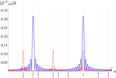
Figure 2: Illustration of the bosonic resonances: The linear coefficients $|\beta^{{}_{(1)}}_{mn}|$ for the bosonic Bogoliubov transformations, are shown for a real, massless scalar field in $(1+1)$ dimensions. The travel scenario has $N$ segments of uniform acceleration $h/\delta$ and duration $\tau/2$ as measured at the cavity’s centre, separated by $(N-1)$ segments of inertial coasting of the same duration (to first order in $h$), as illustrated in Fig. 1 for $N=2$. The curves in Fig. 2 are plotted for $N=15$, $(m,n)=(k,k^{\prime})=(1,2)$ (blue,solid) and $(m,n)=(k^{\prime},k^{\prime\prime})=(2,3)$ (red,dashed) and $u:=h\tau/[4\delta\operatorname{atanh}(h/2)]$. The vertical dashed lines indicate the potential resonance times for $(k,k^{\prime})$ and $(k^{\prime},k^{\prime\prime})$ respectively. The explicit form of the Bogoliubov coefficients can be found in Refs. BruschiFuentesLouko2012 ; BruschiDraganLeeFuentesLouko2012 .

Nonetheless, the entanglement of the four-mode system is genuinely multipartite, which demonstrates once again that genuine multipartite entanglement provides a richer structure than simple combinations of bipartite correlations. Moreover, the responsible coefficient $|\beta^{{}_{(1)}}_{kk^{\prime}}|$ can be resonantly enhanced, within the limitations of the perturbative regime, by appropriate travel scenarios when a massless scalar field is contained within the cavity BruschiDraganLeeFuentesLouko2012 .

Such resonances can occur if the chosen travel scenario consists of $N$ identical building blocks of two or more different, inertial or uniformly-accelerated, trajectory segments. If the overall proper time $\tau$ of one such building block, measured at the centre of the box, satisfies the necessary resonance condition

$$\tau =\tfrac{2\,n\,\delta}{k\,+\,k^{\prime}}\,,$$ (11)

where $n$ is a positive integer, and the coefficient $(\beta_{1})^{{}_{(1)}}_{kk^{\prime}}$ of a single such building block is nonzero, then the corresponding coefficient after $N$ repetitions scales linearly with $N$, i.e.,

$$(\beta_{N})^{{}_{(1)}}_{kk^{\prime}} =N(\beta_{1})^{{}_{(1)}}_{kk^{\prime}}\,.$$ (12)

This scaling is valid within the perturbative regime, i.e., as long as $Nh\ll 1$. A detailed derivation of the condition in Eq.(11) can be found in Ref. BruschiDraganLeeFuentesLouko2012 but the discussion of the continuous variable techniques necessary for the proof lies beyond the scope of this paper. See Fig. 2 for an illustration of the resonances for different mode pairs.

The physical reason for the occurrence of these resonances lies in the phases $G_{m}$ that are acquired by the modes during the free time evolution in the travel segments. The Bogoliubov transformations that switch between segments of inertial and uniformly-accelerated motion act as pairwise two-mode squeezing operations on all modes of opposite parity, see Ref. FriisFuentes2012 ; BruschiDraganLeeFuentesLouko2012 . When at least two such switches are combined to a building block, the magnitude of the corresponding overall squeezing parameter depends on the proper time between these switches as measured at the centre of the cavity. The quantities $G_{m}$ are functions of this time and the mode numbers $m$. In particular, if, and only if, the quantum field in question is massless, all frequencies are integer multiples of some basic frequency and the phases can combine constructively to facilitate the resonance.

II.2 Dirac fields

Let us now consider the analogous scenario for cavities containing fermionic rather than bosonic quantum fields. In particular, let us assume that Alice’s, Rob’s and Charlie’s cavities confine Dirac fields, as discussed in Refs. FriisLeeBruschiLouko2012 ; FriisBruschiLoukoFuentes2012 . In the in-region the field in Rob’s cavity satisfies the Dirac equation $(i\gamma^{\mu}\partial_{\mu}-m)\psi=0$ and the mode functions obey the boundary conditions

$$(\psi^{\,\dagger}_{\omega}\gamma^{0}\gamma^{1}\psi_{\omega^{\prime}})_{x=a}\,=\,(\psi^{\,\dagger}_{\omega}\gamma^{0}\gamma^{1}\psi_{\omega^{\prime}})_{x=b} =0\,.$$ (13)

Here $\gamma^{\mu}$ $(\mu=0,1,2,3)$ are the usual Dirac matrices satisfying the anti-commutation relations $\{\gamma^{\mu},\gamma^{\nu}\}=2\eta^{\mu\nu}$. Due to the boundary conditions the field modes can be labelled by an integer $n$ and the field can be decomposed as

$$\psi=\sum_{n\geq 0}b_{n}\psi_{n}+\sum_{n<0}c_{n}^{\dagger}\psi_{n}\,.$$ (14)

The operators $b_{n}$ and $c_{n}$ annihilate particles and antiparticles respectively. The vacuum state of the cavity is defined by $b_{n}\left|\!\left|\right.\right.\!0\!\left.\left.\right\rangle\!\right\rangle=c_{n}\left|\!\left|\right.\right.\!0\!\left.\left.\right\rangle\!\right\rangle=0\ \forall n$, while the single particle and antiparticle states, $\left|\!\left|\right.\right.\!\!1_{m}\!\!\left.\left.\right\rangle\!\right\rangle^{\!\!+}$ and $\left|\!\left|\right.\right.\!\!1_{n}\!\!\left.\left.\right\rangle\!\right\rangle^{\!\!-}$, are created from the vacuum by $b_{m}^{\dagger}$ and $c_{n}^{\dagger}$ respectively. The fermionic operators further satisfy $\{b_{m},b_{n}^{\dagger}\}=\{c_{m},c_{n}^{\dagger}\}=\delta_{mn}$, while all other anti-commutators vanish.

In analogy to the bosonic states (3) we select initially bipartite entangled fermionic states that correlate the cavities of Alice and Rob, as well as Rob and Charlie respectively, i.e.,

$$\left|\!\left|\right.\right.\!\phi^{\pm}\!\left.\left.\right\rangle\!\right\rangle_{AR} =\tfrac{1}{\sqrt{2}}\,\bigl{(}\,\left|\!\left|\right.\right.\!0\!\left.\left.\right\rangle\!\right\rangle\,\pm\,\left|\!\left|\right.\right.\!\!1_{A}\!\!\left.\left.\right\rangle\!\right\rangle^{\!\!-}\,\left|\!\left|\right.\right.\!\!1_{\kappa}\!\!\left.\left.\right\rangle\!\right\rangle^{\!\!+}\,\bigr{)}\,,$$ (15a)

$$\left|\!\left|\right.\right.\!\phi^{\pm}\!\left.\left.\right\rangle\!\right\rangle_{RC} =\tfrac{1}{\sqrt{2}}\,\bigl{(}\,\left|\!\left|\right.\right.\!0\!\left.\left.\right\rangle\!\right\rangle\,\pm\,\left|\!\left|\right.\right.\!\!1_{\kappa^{\prime}}\!\!\left.\left.\right\rangle\!\right\rangle^{\!\!-}\,\left|\!\left|\right.\right.\!\!1_{C}\!\!\left.\left.\right\rangle\!\right\rangle^{\!\!+}\,\bigr{)}\,,$$ (15b)

where we have chosen particle and antiparticle modes in agreement with charge superselection rules. The multi-particle states in Eq. (15) are elements of anti-symmetrized tensor product spaces of single particle mode functions $\psi_{i}$, i.e.,

$$\left|\!\left|\right.\right.\!\!1_{p}\!\!\left.\left.\right\rangle\!\right\rangle^{\!\!+}\,\left|\!\left|\right.\right.\!\!1_{q}\!\!\left.\left.\right\rangle\!\right\rangle^{\!\!-} :=\left|\!\left|\right.\right.\!\!\psi_{p}\!\!\left.\left.\right\rangle\!\right\rangle^{\!\!+}\!\wedge\left|\!\left|\right.\right.\!\!\psi_{q}\!\!\left.\left.\right\rangle\!\right\rangle^{\!\!-}\,:=\,b^{\dagger}_{p}c^{\dagger}_{q}\,\left|\!\left|\right.\right.\!0\!\left.\left.\right\rangle\!\right\rangle\,,$$ (16)

where $A\wedge B=(A\otimes B-B\otimes A)/\sqrt{2}$ denotes the anti-symmetrized tensor product. For the purpose of quantum information procedures one can map this “wedge product” structure to the usual tensor product structure by defining a convention for partial tracing. Our choice here is to trace out operators “from the inside”, i.e.,

$$\textnormal{Tr}_{p}\Bigl{(}b^{\dagger}_{\kappa}b^{\dagger}_{p}\,\left|\!\left|\right.\right.\!0\!\left.\left.\right\rangle\!\right\rangle\left\langle\!\left\langle\right.\right.\!0\!\left.\left.\right|\!\right|\,b_{p}\Bigr{)} =\,b^{\dagger}_{\kappa}\,\left|\!\left|\right.\right.\!0\!\left.\left.\right\rangle\!\right\rangle\left\langle\!\left\langle\right.\right.\!0\!\left.\left.\right|\!\right|\,.$$ (17)

In the spirit of this convention we reverse the ordering of the states in the adjoint space, i.e., $\left\langle\!\left\langle\right.\right.\!0\!\left.\left.\right|\!\right|b_{p}b_{\kappa}=^{\,+\!\!\!}\left\langle\!\left\langle\right.\right.\!\!1_{p}\!\!\left.\left.\right|\!\right|\!^{\,+\!\!\!}\left\langle\!\left\langle\right.\right.\!\!1_{\kappa}\!\!\left.\left.\right|\!\right|$. Different conventions can generally introduce ambiguities in the resulting fermionic states, which has been the subject of an on-going debate, see Ref. AmbiguityDebate . However, we have verified that no ambiguities appear in our results to second order in the perturbative calculations. For the symmetrized tensor product structure of bosonic modes analogous mappings have to be performed. However, no sign ambiguities occur for bosons and the results are therefore independent of the chosen mapping.

The Bogoliubov transformation that relates the in-region modes $\psi_{n}$ and the out-region modes $\tilde{\psi}_{m}$ is given by

$$\tilde{\psi}_{m} =\sum\limits_{n}\mathcal{A}_{mn}\psi_{n}$$ (18)

where $n\in\mathds{Z}$ and the fermionic Bogoliubov coefficients can be expanded in a Maclaurin series in the parameter $h$ as

$$\mathcal{A}_{mn} =\,\mathcal{A}_{mn}^{{}_{(0)}}+\mathcal{A}_{mn}^{{}_{(1)}}+O(h^{2})\,,$$ (19)

where the superscript ${}^{{}_{(n)}}$ again denotes the power of $h$, and we have $\mathcal{A}^{{}_{(1)}}_{nn}=0$ and $\mathcal{A}^{{}_{(0)}}_{mn}=\delta_{mn}G_{m}$ (no summation). In the fermionic case the subscripts $m$ and $n$ can take positive as well as negative values, representing particle and antiparticle modes respectively. Furthermore, the splitting into particle and antiparticle modes is controlled by an additional parameter in the Bogoliubov coefficients, see Ref. FriisLeeBruschiLouko2012 . We set this parameter to zero, in which case the phase factors $G_{m}$ coincide for bosons and fermions.

We continue, as previously, by transforming the initial state $\left|\!\left|\right.\right.\!\!\Phi^{\pm}\!\!\left.\left.\right\rangle\!\right\rangle=\left|\!\left|\right.\right.\!\!\phi^{\pm}\!\!\left.\left.\right\rangle\!\right\rangle_{A\kappa}\left|\!\left|\right.\right.\!\!\phi^{\pm}\!\!\left.\left.\right\rangle\!\right\rangle_{\kappa^{\prime}C}$ with the corresponding density operator $\varrho^{\,\pm}_{A\!RC}=\left|\!\left|\right.\right.\!\!\Phi^{\pm}\!\!\left.\left.\right\rangle\!\right\rangle\left\langle\!\left\langle\right.\right.\!\!\Phi^{\pm}\!\!\left.\left.\right|\!\right|$, to the out-region states, i.e., we use the series expansions FriisLeeBruschiLouko2012

$$\left|\!\left|\right.\right.\!0\!\left.\left.\right\rangle\!\right\rangle\ \; =\left|\!\left|\right.\right.\!\tilde{0}\!\left.\left.\right\rangle\!\right\rangle\,+\,\sum_{p,q}\,G_{q}^{\,*}\mathcal{A}^{{}_{(1)}\raisebox{-1.7pt}{\scriptsize{$*$}}}_{pq}\,\tilde{b}_{p}^{\dagger}\tilde{c}_{q}^{\dagger}\,\left|\!\left|\right.\right.\!\tilde{0}\!\left.\left.\right\rangle\!\right\rangle\,+\,O(h^{2})\,,$$ (20a)

$$\left|\!\left|\right.\right.\!\!1_{\kappa}\!\!\left.\left.\right\rangle\!\right\rangle^{\!\!+}\, =G^{\,*}_{\kappa}\left|\!\left|\right.\right.\!\!\tilde{1}_{\kappa}\!\!\left.\left.\right\rangle\!\right\rangle^{\!\!+}\,+\,\sum_{m\geq 0}\,\mathcal{A}^{{}_{(1)}\raisebox{-1.7pt}{\scriptsize{$*$}}}_{m\kappa}\,\,\left|\!\left|\right.\right.\!\!\tilde{1}_{m}\!\!\left.\left.\right\rangle\!\right\rangle^{\!\!+}$$ (20b)

$$\ \ +\,G_{\kappa}^{\,*}\sum\limits_{p,q}\,G_{q}^{\,*}\mathcal{A}^{{}_{(1)}\raisebox{-1.7pt}{\scriptsize{$*$}}}_{pq}\,\tilde{b}_{p}^{\dagger}\tilde{c}_{q}^{\dagger}\,\left|\!\left|\right.\right.\!\!\tilde{1}_{\kappa}\!\!\left.\left.\right\rangle\!\right\rangle^{\!\!+}\,+\,O(h^{2})\,,$$

$$\left|\!\left|\right.\right.\!\!1_{\kappa^{\prime}}\!\!\left.\left.\right\rangle\!\right\rangle^{\!\!-} =G_{\kappa^{\prime}}\left|\!\left|\right.\right.\!\!\tilde{1}_{\kappa^{\prime}}\!\!\left.\left.\right\rangle\!\right\rangle^{\!\!-}\,+\,\sum_{n<0}\,\mathcal{A}^{{}_{(1)}}_{n\kappa^{\prime}}\,\,\left|\!\left|\right.\right.\!\!\tilde{1}_{n}\!\!\left.\left.\right\rangle\!\right\rangle^{\!\!-}$$ (20c)

$$\ \ +\,G_{\kappa^{\prime}}\sum\limits_{p,q}\,G_{q}^{\,*}\mathcal{A}^{{}_{(1)}\raisebox{-1.7pt}{\scriptsize{$*$}}}_{pq}\,\tilde{b}_{p}^{\dagger}\tilde{c}_{q}^{\dagger}\,\left|\!\left|\right.\right.\!\!\tilde{1}_{\kappa^{\prime}}\!\!\left.\left.\right\rangle\!\right\rangle^{\!\!-}\,+\,O(h^{2})\,,$$

$$\left|\!\left|\right.\right.\!\!1_{\kappa}\!\!\left.\left.\right\rangle\!\right\rangle^{\!\!+}\!\left|\!\left|\right.\right.\!\!1_{\kappa^{\prime}}\!\!\left.\left.\right\rangle\!\right\rangle^{\!\!-} \,=G_{\kappa^{\prime}}G_{\kappa}^{\,*}\left|\!\left|\right.\right.\!\!\tilde{1}_{\kappa}\!\!\left.\left.\right\rangle\!\right\rangle^{\!\!+}\!\left|\!\left|\right.\right.\!\!\tilde{1}_{\kappa^{\prime}}\!\!\left.\left.\right\rangle\!\right\rangle^{\!\!-}\,+\,G_{\kappa^{\prime}}\mathcal{A}^{{}_{(1)}\raisebox{-1.7pt}{\scriptsize{$*$}}}_{\kappa^{\prime}\kappa}\,\left|\!\left|\right.\right.\!\tilde{0}\!\left.\left.\right\rangle\!\right\rangle$$

$$\ +\,G_{\kappa^{\prime}}G_{\kappa}^{\,*}\sum_{p,q}\,G_{q}^{\,*}\mathcal{A}^{{}_{(1)}\raisebox{-1.7pt}{\scriptsize{$*$}}}_{pq}\,\tilde{b}_{p}^{\dagger}\tilde{c}_{q}^{\dagger}\,\left|\!\left|\right.\right.\!\!\tilde{1}_{\kappa}\!\!\left.\left.\right\rangle\!\right\rangle^{\!\!+}\!\left|\!\left|\right.\right.\!\!\tilde{1}_{\kappa^{\prime}}\!\!\left.\left.\right\rangle\!\right\rangle^{\!\!-}$$

$$\ +\,G_{\kappa^{\prime}}\sum\limits_{m\geq 0}\mathcal{A}^{{}_{(1)}\raisebox{-1.7pt}{\scriptsize{$*$}}}_{m\kappa^{\prime}}\,\left|\!\left|\right.\right.\!\!\tilde{1}_{m}\!\!\left.\left.\right\rangle\!\right\rangle^{\!\!+}\!\left|\!\left|\right.\right.\!\!\tilde{1}_{\kappa^{\prime}}\!\!\left.\left.\right\rangle\!\right\rangle^{\!\!-}$$ (20d)

$$\ +\,G_{\kappa}^{\,*}\sum\limits_{n<0}\mathcal{A}^{{}_{(1)}}_{n\kappa^{\prime}}\,\left|\!\left|\right.\right.\!\!\tilde{1}_{\kappa}\!\!\left.\left.\right\rangle\!\right\rangle^{\!\!+}\!\left|\!\left|\right.\right.\!\!\tilde{1}_{n}\!\!\left.\left.\right\rangle\!\right\rangle^{\!\!-}\,+\,O(h^{2})\,,$$

where we have used the convention from Eqs. (16,17), to obtain the transformed state $\tilde{\varrho}^{\,\pm}_{A\!RC}$.

Subsequently we trace over all particle and antiparticle modes except $\kappa\geq 0$ and $\kappa^{\prime}<0$, which leaves us with the reduced state $\tilde{\varrho}^{\,\pm}_{A\kappa\kappa^{\prime}C}$. To first order in the parameter $h$ no new diagonal elements are generated in the state transformation, which makes it easy to identify an inequality that acts as a witness for genuine multipartite entanglement. However, due to the Pauli exclusion principle, we cannot employ a witnesses of the type of Eq. (8) for the fermionic system. Instead we construct the witness

$$\left|{}^{\raisebox{0.7pt}{\scriptsize{$-$}}\!\!\!}\left\langle\!\left\langle\right.\right.\!\!\tilde{1}_{\kappa^{\prime}}\!\!\left.\left.\right|\!\right|^{\,+\!\!\!}\left\langle\!\left\langle\right.\right.\!\!\tilde{1}_{\kappa}\!\!\left.\left.\right|\!\right|\tilde{\varrho}^{\,\pm}_{A\kappa\kappa^{\prime}C}\left|\!\left|\right.\right.\!\!\tilde{1}_{\kappa^{\prime}}\!\!\left.\left.\right\rangle\!\right\rangle^{\!\!-}\left|\!\left|\right.\right.\!\!1_{C}\!\!\left.\left.\right\rangle\!\right\rangle^{\!\!+}\right|$$ (21)

$$\,+\, \left|{}^{\raisebox{0.7pt}{\scriptsize{$+$}}\!\!\!}\left\langle\!\left\langle\right.\right.\!\!1_{C}\!\!\left.\left.\right|\!\right|^{-\!\!\!}\left\langle\!\left\langle\right.\right.\!\!1_{A}\!\!\left.\left.\right|\!\right|\tilde{\varrho}^{\,\pm}_{A\kappa\kappa^{\prime}C}\left|\!\left|\right.\right.\!\!\tilde{1}_{\kappa^{\prime}}\!\!\left.\left.\right\rangle\!\right\rangle^{\!\!-}\left|\!\left|\right.\right.\!\!1_{C}\!\!\left.\left.\right\rangle\!\right\rangle^{\!\!+}\right|\,-\,O(h^{2})\,\leq 0\,,$$

which we can express as

$$\tfrac{1}{2}|\mathcal{A}^{{}_{(1)}}_{\kappa\kappa^{\prime}}|\,-\,O(h^{2})\, \leq 0\,.$$ (22)

The complete form of the witness can be found in the appendix, see Eq. (32). As with its bosonic counterpart (9) the inequality (22) is always violated if the modes $\kappa$ and $\kappa^{\prime}$ have opposite parity, in which case $\mathcal{A}^{{}_{(1)}}_{\kappa\kappa^{\prime}}\neq 0$. In the case where $(\kappa+\kappa^{\prime})$ is even the first order coefficient vanishes identically, see Ref. FriisLeeBruschiLouko2012 , and the usefulness of the witness has to be evaluated for each selection of mode numbers and travel scenarios individually.

The witness employed in Eq. (22) is again a lower bound to the minimal average mutual information across any bipartition WuKampermannBruszKloecklHuber2012 , although, this time, it is not tight for pure states as Eq. (8). However, there are other conceptually intriguing features appearing for the fermionic four-qubit state $\tilde{\varrho}^{\,\pm}_{A\kappa\kappa^{\prime}C}$. First, we notice that the unperturbed reduced density operators $\varrho^{\,\pm}_{AC}$ and $\varrho^{\,\pm}_{\kappa\kappa^{\prime}}$ are both maximally mixed. This means that, in contrast to the bosonic case, no bipartite entanglement between the fermionic modes $\kappa$ and $\kappa^{\prime}$ can be generated from the initial state $\varrho^{\,\pm}_{A\!RC}$ by small perturbations. The negativity, which is nonzero for all entangled two-qubit states, requires (at least) one of the degenerate eigenvalues $1/4$ of the partial transpose to become negative. This cannot happen within the perturbative regime. This behaviour can be readily understood in terms of the monogamy of entanglement (see, e.g., Ref. OsborneVerstraete2006 ): To first order in the small parameter expansion the reduced states of the initially maximally entangled modes, $A$ and $\kappa$ or $\kappa^{\prime}$ and $C$, respectively, remain unperturbed up to relative phases due to the time evolution. In particular, the bipartite entanglement between $A$ and $\kappa$, as well as between $\kappa^{\prime}$ and $C$ is maximal to first order in $h$, see Ref. FriisLeeBruschiLouko2012 , which excludes the possibility of first order correlations between $\kappa$ and $\kappa^{\prime}$. This remarkable difference between the scalar field and the Dirac field highlights once more (see, e.g., Refs. AlsingFuentes-SchullerMannTessier2006 ; AdessoFuentes-SchullerEricsson2007 ; AdessoFuentes-Schuller2009 ) the contrast of fermionic and bosonic particle statistics in the context of Bogoliubov transformations.

Furthermore, we can straightforwardly classify the entanglement of the four qubit state. We notice that, to first order, the state $\tilde{\varrho}^{\,\pm}_{A\kappa\kappa^{\prime}C}$ can be decomposed as

$$\tilde{\varrho}^{\,\pm}_{A\kappa\kappa^{\prime}C} =\left|\!\left|\right.\right.\!\!\mathcal{D}\!\!\left.\left.\right\rangle\!\right\rangle\left\langle\!\left\langle\right.\right.\!\!\mathcal{D}\!\!\left.\left.\right|\!\right|\,+\,O(h^{2})$$ (23)

where $\left|\!\left|\right.\right.\!\mathcal{D}\!\left.\left.\right\rangle\!\right\rangle$ is a Dicke state Dicke1954 ; HuberErkerSchimpfGabrielHiesmayr2011 , given by

$$\left|\!\left|\right.\right.\!\!\mathcal{D}\!\!\left.\left.\right\rangle\!\right\rangle =\tfrac{1}{2}\bigl{(}\,\left|\!\left|\right.\right.\!\tilde{0}\!\left.\left.\right\rangle\!\right\rangle\,\pm\,G^{\,*}_{\kappa}\left|\!\left|\right.\right.\!\!1_{A}\!\!\left.\left.\right\rangle\!\right\rangle^{\!\!-}\!\left|\!\left|\right.\right.\!\!\tilde{1}_{\kappa}\!\!\left.\left.\right\rangle\!\right\rangle^{\!\!+}\,\pm\,G_{\kappa^{\prime}}\left|\!\left|\right.\right.\!\!\tilde{1}_{\kappa^{\prime}}\!\!\left.\left.\right\rangle\!\right\rangle^{\!\!-}\!\left|\!\left|\right.\right.\!\!1_{C}\!\!\left.\left.\right\rangle\!\right\rangle^{\!\!+}$$

$$\ +\,G_{\kappa^{\prime}}\mathcal{A}^{{}_{(1)}\raisebox{-1.7pt}{\scriptsize{$*$}}}_{\kappa\kappa^{\prime}}\left|\!\left|\right.\right.\!\!\tilde{1}_{\kappa}\!\!\left.\left.\right\rangle\!\right\rangle^{\!\!+}\!\left|\!\left|\right.\right.\!\!\tilde{1}_{\kappa^{\prime}}\!\!\left.\left.\right\rangle\!\right\rangle^{\!\!-}\,-\,G^{\,*}_{\kappa}\mathcal{A}^{{}_{(1)}}_{\kappa\kappa^{\prime}}\left|\!\left|\right.\right.\!\!1_{A}\!\!\left.\left.\right\rangle\!\right\rangle^{\!\!-}\!\left|\!\left|\right.\right.\!\!1_{C}\!\!\left.\left.\right\rangle\!\right\rangle^{\!\!+}$$

$$\ -\,G^{\,*}_{\kappa}G_{\kappa^{\prime}}\left|\!\left|\right.\right.\!\!1_{A}\!\!\left.\left.\right\rangle\!\right\rangle^{\!\!-}\!\left|\!\left|\right.\right.\!\!\tilde{1}_{\kappa}\!\!\left.\left.\right\rangle\!\right\rangle^{\!\!+}\!\left|\!\left|\right.\right.\!\!\tilde{1}_{\kappa^{\prime}}\!\!\left.\left.\right\rangle\!\right\rangle^{\!\!-}\!\left|\!\left|\right.\right.\!\!1_{C}\!\!\left.\left.\right\rangle\!\right\rangle^{\!\!+}\,\bigr{)}\,,$$ (24)

where $G_{m}$ are mode dependent phase factors of unit magnitude, i.e., $|G_{m}|=1$, that are determined by the specific travel scenario, see, e.g., Ref. FriisLeeBruschiLouko2012 . The usual form of the Dicke state can be obtained from Eq. (23) by local unitaries, e.g., bit-flips in the modes $A$ and $\kappa^{\prime}$.

III Single-cavity entanglement

Let us now modify our previous setup and consider only Rob’s cavity on its own, as in Ref. FriisBruschiLoukoFuentes2012 . In particular, let us assume for simplicity that the initial state of the in-region modes in that cavity is the vacuum. We want to investigate the genuine multipartite correlations that might possibly be generated between three selected modes by performing a Bogoliubov transformation to the out-region modes.

III.1 Scalar fields

The in-region vacuum $\left|\right.0\left.\right\rangle$ of a real scalar field $\phi$ can be related to the out-region vacuum $\left|\right.\tilde{0}\left.\right\rangle$ by $\left|\right.0\left.\right\rangle=Me^{W}\left|\right.\tilde{0}\left.\right\rangle$, where $M$ is a normalization constant and $W:=\tfrac{1}{2}\sum_{i,j}V_{ij}\tilde{a}_{i}^{\dagger}\tilde{a}_{j}^{\dagger}$. The coefficients $V_{ij}$ form a symmetric matrix that can be expressed as $V=-\beta^{\,*}\alpha^{-1}$, where $\beta=(\beta_{mn})$ and it is implicitly assumed that $\alpha=(\alpha_{mn})$ is invertible. We then apply the small parameter expansion for the Bogoliubov coefficients and find $V=V^{\raisebox{0.7pt}{\tiny{$(1)$}}}+O(h^{2})$ and the normalization constant $M=(1-\tfrac{1}{4}\sum_{i,j}|V_{ij}|^{2})+O(h^{3})$, see Ref. FriisBruschiLoukoFuentes2012 .

Having transformed the initial vacuum state $\left|\right.0\left.\right\rangle$ to the out-region, we continue by tracing over all out-region modes except three chosen modes $k$, $k^{\prime}$ and $k^{\prime\prime}$. We denote the transformed, reduced state by $\tilde{\rho}_{k\,k^{\prime}k^{\prime\prime}}$, where we keep terms up to second order in $h$. At this stage we further assume that the modes do not all have the same parity, e.g., let us choose $(k-k^{\prime})$ and $(k^{\prime}-k^{\prime\prime})$ to be odd, which implies $(k-k^{\prime\prime})$ is even. This further means that $|\,\beta^{{}_{(1)}}_{k\,k^{\prime}}|\geq 0$, $|\,\beta^{{}_{(1)}}_{k^{\prime}k^{\prime\prime}}|\geq 0$, while $|\,\beta^{{}_{(1)}}_{k\,k^{\prime\prime}}|=0$. With this convention in mind we select a witness for genuine multipartite entanglement, i.e.,

$$2\,|\left\langle\right.\tilde{0}\left.\right|\,\tilde{\rho}_{k\,k^{\prime}k^{\prime\prime}}\,\left|\right.\!\tilde{1}_{k}\!\left.\right\rangle\left|\right.\!\tilde{2}_{k^{\prime}}\!\left.\right\rangle\left|\right.\!\tilde{1}_{k^{\prime\prime}}\!\left.\right\rangle|\,-\,O(h^{3}) \leq 0\,,$$ (25)

which can be rewritten as

$$2\sqrt{2}\,|\,\beta^{{}_{(1)}}_{k\,k^{\prime}}|\,|\,\beta^{{}_{(1)}}_{k^{\prime}k^{\prime\prime}}|\,-\,O(h^{3}) \leq 0\,.$$ (26)

As previously, the witness (25) presents a lower bound to the convex roof extension of the minimal average mutual information across all bi-partitions WuKampermannBruszKloecklHuber2012 and its complete form is given by (33) of the appendix. It can be immediately noticed that that the previously discussed bosonic resonances BruschiDraganLeeFuentesLouko2012 allow the linear enhancement of the individual coefficients, $|\,\beta^{{}_{(1)}}_{k\,k^{\prime}}|$ or $|\,\beta^{{}_{(1)}}_{k^{\prime}k^{\prime\prime}}|$, for particular basic travel times $\tau=2n\delta/(k+k^{\prime})$ and $\tau=2m\delta/(k^{\prime}+k^{\prime\prime})$, $n,m\in\mathds{N}_{\!+}$, respectively. Interestingly, these resonances coincide for $n=p(k+k^{\prime})$ and $m=p(k^{\prime}+k^{\prime\prime})$, i.e., when the travel time, as measured at the centre of the cavity, for a single cycle of the repeated basic travel scenario is $\tau=2p\delta$, $p\in\mathds{N}_{\!+}$, see Fig. 2.

At this mode-independent resonance the lower bound on the genuine multipartite entanglement increases quadratically with the number $N$ of repetitions of the basic travel block. At the same time the mixedness that is introduced to the system by tracing out the other modes contains second order terms $f^{\beta}_{k\lnot k^{\prime}}$, $f^{\beta}_{k^{\prime}\lnot k,k^{\prime\prime}}$ and $f^{\beta}_{k^{\prime\prime}\lnot k^{\prime}}$, where $f^{\beta}_{m\lnot p}=\tfrac{1}{2}\sum_{n\neq p}|\,\beta^{{}_{(1)}}_{mn}|^{2}$, which all exhibit quadratic scaling at the mode-independent resonance. The validity of the perturbative approach is ensured since all second order terms are at most proportional to $N^{2}h^{2}\ll Nh$.

However, the classification of the bosonic genuine multipartite correlations remains an unsolved problem. To first order the transformed state can be written as a pure Dicke state HuberErkerSchimpfGabrielHiesmayr2011 , but since the genuine multipartite entanglement is detected at second order this is of no significance. To second order the modes effectively become qutrits, for which generally little is known about entanglement classes.

III.2 Dirac fields

Let us again consider the fermionic counterpart to the bosonic situation. The in-region vacuum $\left|\!\left|\right.\right.\!0\!\left.\left.\right\rangle\!\right\rangle$ of the Dirac field $\psi$ is related to the out-region vacuum $\left|\!\left|\right.\right.\!\tilde{0}\!\left.\left.\right\rangle\!\right\rangle$ by $\left|\!\left|\right.\right.\!0\!\left.\left.\right\rangle\!\right\rangle=\mathcal{M}e^{\mathcal{W}}\left|\!\left|\right.\right.\!\tilde{0}\!\left.\left.\right\rangle\!\right\rangle$, where $\mathcal{W}:=\sum_{\begin{subarray}{c}\mbox{\tiny{$p\!\geq\!0$}}\\ \mbox{\tiny{$q\!<\!0$}}\end{subarray}}\mathcal{V}_{pq}b^{\dagger}_{p}c^{\dagger}_{q}$ and $\mathcal{M}$ is a normalization constant. Working perturbatively in the parameter $h$ the coefficient matrix $\mathcal{V}$ can be expanded in a Maclaurin series as $\mathcal{V}=\mathcal{V}^{\raisebox{0.7pt}{\tiny{$(1)$}}}+O(h^{2})$ and $\mathcal{V}^{{}_{(1)}}_{pq}=G_{q}\mathcal{A}^{{}_{(1)}\raisebox{-1.7pt}{\scriptsize{$*$}}}_{pq}$ (no summation), where the $G_{m}$ are mode specific phase factors, i.e., $|G_{m}|=1$, that depend on the chosen travel scenario, see Ref. FriisLeeBruschiLouko2012 . The normalization constant can be found to be $\mathcal{M}=1-\tfrac{1}{2}\sum_{\begin{subarray}{c}\mbox{\tiny{$p\!\geq\!0$}}\\ \mbox{\tiny{$q\!<\!0$}}\end{subarray}}|\mathcal{V}^{{}_{(1)}}_{pq}|^{2}+O(h^{3})$.

We can then perform the Bogoliubov transformation of the in-region vacuum $\left|\!\left|\right.\right.\!0\!\left.\left.\right\rangle\!\right\rangle$ to the out-region state and trace over all modes except three chosen modes $\kappa\geq 0$, $\kappa^{\prime}\geq 0$ and $\kappa^{\prime\prime}<0$, obtaining the state $\tilde{\varrho}_{\kappa\,\kappa^{\prime}\kappa^{\prime\prime}}$. Since we do not expect any coherence effects between modes of the same charge when we start from the vacuum, see Ref. FriisBruschiLoukoFuentes2012 , we further assume that $(\kappa+\kappa^{\prime})$ is even, while $(\kappa+\kappa^{\prime\prime})$ and $(\kappa^{\prime}+\kappa^{\prime\prime})$ are odd. Specializing to the massless case this implies that $|\mathcal{A}^{{}_{(1)}}_{\kappa\kappa^{\prime\prime}}|\geq 0$ and $|\mathcal{A}^{{}_{(1)}}_{\kappa^{\prime}\kappa^{\prime\prime}}|\geq 0$, while $|\mathcal{A}^{{}_{(1)}}_{\kappa\kappa^{\prime}}|=0$.

For the state $\tilde{\varrho}_{\kappa\,\kappa^{\prime}\kappa^{\prime\prime}}$ we can form a witness for genuine multipartite entanglement using the techniques from Ref. HuberMintertGabrielHiesmayr2010 . The violation of the inequality

$$|\left\langle\!\left\langle\right.\right.\!\tilde{0}\!\left.\left.\right|\!\right|\tilde{\varrho}_{\kappa\,\kappa^{\prime}\kappa^{\prime\prime}}\left|\!\left|\right.\right.\!\!\tilde{1}_{\kappa}\!\!\left.\left.\right\rangle\!\right\rangle^{\!\!+}\left|\!\left|\right.\right.\!\!\tilde{1}_{\kappa^{\prime\prime}}\!\!\left.\left.\right\rangle\!\right\rangle^{\!\!-}|+|\left\langle\!\left\langle\right.\right.\!\tilde{0}\!\left.\left.\right|\!\right|\tilde{\varrho}_{\kappa\,\kappa^{\prime}\kappa^{\prime\prime}}\left|\!\left|\right.\right.\!\!\tilde{1}_{\kappa^{\prime}}\!\!\left.\left.\right\rangle\!\right\rangle^{\!\!+}\left|\!\left|\right.\right.\!\!\tilde{1}_{\kappa^{\prime\prime}}\!\!\left.\left.\right\rangle\!\right\rangle^{\!\!-}|$$

$$-\Bigl{[}\left\langle\!\left\langle\right.\right.\!\tilde{0}\!\left.\left.\right|\!\right|\tilde{\varrho}_{\kappa\,\kappa^{\prime}\kappa^{\prime\prime}}\left|\!\left|\right.\right.\!\tilde{0}\!\left.\left.\right\rangle\!\right\rangle\Bigl{(}^{\raisebox{-3.3pt}{\tiny{$-$}}\!\!}\left\langle\!\left\langle\right.\right.\!\!\tilde{1}_{\kappa^{\prime\prime}}\!\!\left.\left.\right|\!\right|^{\!+\!\!}\left\langle\!\left\langle\right.\right.\!\!\tilde{1}_{\kappa}\!\!\left.\left.\right|\!\right|\tilde{\varrho}_{\kappa\,\kappa^{\prime}\kappa^{\prime\prime}}\left|\!\left|\right.\right.\!\!\tilde{1}_{\kappa}\!\!\left.\left.\right\rangle\!\right\rangle^{\!\!+}\left|\!\left|\right.\right.\!\!\tilde{1}_{\kappa^{\prime\prime}}\!\!\left.\left.\right\rangle\!\right\rangle^{\!\!-}$$

$$+^{-\!\!\!\!}\left\langle\!\left\langle\right.\right.\!\!\tilde{1}_{\kappa^{\prime\prime}}\!\!\left.\left.\right|\!\right|^{+\!\!\!}\left\langle\!\left\langle\right.\right.\!\!\tilde{1}_{\kappa^{\prime}}\!\!\left.\left.\right|\!\right|\tilde{\varrho}_{\kappa\,\kappa^{\prime}\kappa^{\prime\prime}}\left|\!\left|\right.\right.\!\!\tilde{1}_{\kappa^{\prime}}\!\!\left.\left.\right\rangle\!\right\rangle^{\!\!+}\left|\!\left|\right.\right.\!\!\tilde{1}_{\kappa^{\prime\prime}}\!\!\left.\left.\right\rangle\!\right\rangle^{\!\!-}\Bigr{)}\Bigr{]}^{\raisebox{-0.5pt}{\tiny{$\tfrac{1}{2}$}}}-O(h^{2})\leq 0$$ (27)

detects genuine multipartite entanglement. The complete form without perturbative expansion is given by Eq. (34) in the appendix. It can be expressed in the simple form

$$|\mathcal{A}^{{}_{(1)}}_{\kappa\kappa^{\prime\prime}}|+|\mathcal{A}^{{}_{(1)}}_{\kappa^{\prime}\kappa^{\prime\prime}}|-\sqrt{|\mathcal{A}^{{}_{(1)}}_{\kappa\kappa^{\prime\prime}}|^{2}+|\mathcal{A}^{{}_{(1)}}_{\kappa^{\prime}\kappa^{\prime\prime}}|^{2}}+O(h^{2})\leq 0\,.$$ (28)

Using the triangle inequality this can be easily seen to be violated whenever both $\mathcal{A}^{{}_{(1)}}_{\kappa\kappa^{\prime\prime}}$ and $\mathcal{A}^{{}_{(1)}}_{\kappa^{\prime}\kappa^{\prime\prime}}$ are nonzero.

We can further classify the genuine multipartite entanglement in this case, since the state $\tilde{\varrho}_{\kappa\,\kappa^{\prime}\kappa^{\prime\prime}}$ admits the decomposition

$$\tilde{\varrho}_{\kappa\,\kappa^{\prime}\kappa^{\prime\prime}} =\,\left|\!\left|\right.\right.\!\!\mathrm{W}\!\!\left.\left.\right\rangle\!\right\rangle\left\langle\!\left\langle\right.\right.\!\!\mathrm{W}\!\!\left.\left.\right|\!\right|+O(h^{2})$$ (29)

where the class-defining $W$-state is

$$\left|\!\left|\right.\right.\!\!\mathrm{W}\!\!\left.\left.\right\rangle\!\right\rangle =\,\left|\!\left|\right.\right.\!\tilde{0}\!\left.\left.\right\rangle\!\right\rangle\,+\,G_{\kappa^{\prime\prime}}\mathcal{A}_{\kappa^{\prime}\kappa^{\prime\prime}}^{{}_{(1)}\raisebox{-1.7pt}{\scriptsize{$*$}}}\,\left|\!\left|\right.\right.\!\!\tilde{1}_{\kappa^{\prime}}\!\!\left.\left.\right\rangle\!\right\rangle^{\!\!+}\left|\!\left|\right.\right.\!\!\tilde{1}_{\kappa^{\prime\prime}}\!\!\left.\left.\right\rangle\!\right\rangle^{\!\!-}$$

$$\ \,+\,G_{\kappa^{\prime\prime}}\mathcal{A}_{\kappa\kappa^{\prime\prime}}^{{}_{(1)}\raisebox{-1.7pt}{\scriptsize{$*$}}}\,\left|\!\left|\right.\right.\!\!\tilde{1}_{\kappa}\!\!\left.\left.\right\rangle\!\right\rangle^{\!\!+}\left|\!\left|\right.\right.\!\!\tilde{1}_{\kappa^{\prime\prime}}\!\!\left.\left.\right\rangle\!\right\rangle^{\!\!-}\,.$$ (30)

IV Conclusions

We have studied genuine multipartite entanglement of bosonic and fermionic modes of relativistic quantum fields in non-uniformly moving cavities. We have used the perturbative approach of Refs. BruschiFuentesLouko2012 ; FriisLeeBruschiLouko2012 to handle the Bogoliubov transformations that feature in the transformation of the cavity modes between the inertial in-region and out-region. The non-uniform motion in between these regions populates modes and shifts pre-existing excitations. The final out-region states of a set of chosen modes is then obtained by tracing over all other modes. In two qualitatively different scenarios we have shown that genuine multipartite correlations are generated from initially bi-separable or separable states of the chosen modes.

We have employed witnesses for multipartite entanglement that prove to be advantageous with respect to usual entropic measures in the perturbative regime. The witnesses for the bosonic correlations provide lower bounds to measures of genuine multipartite entanglement that are based on convex roof extensions of the minimal average mutual information over all bi-partitions WuKampermannBruszKloecklHuber2012 . We find that the numerical value of the perturbative corrections to these lower bounds can be resonantly enhanced for any chosen triple of bosonic modes with varying parities. However, the classification of the arising correlations is hindered by the unknown classification structure beyond qubits.

For the fermionic systems, on the other hand, we can detect the genuine multipartite entanglement in the transformed states and, subsequently, assign the entangled states originating from initially bi-separable and separable states to the classes of 4-qubit Dicke states, which can be used in quantum secret sharing  GaertnerKurtsieferBourennaneWeinfurter2007 , and 3-qubit $W$-states respectively.

The creation of specific entangled states in our setup can be considered as the realization of quantum gates by motion in spacetime. In particular, we complement the findings of Refs. FriisFuentes2012 ; BruschiDraganLeeFuentesLouko2012 , where two-mode squeezing gates are implemented as a result of the non-uniform cavity motion, with the creation of the Dicke and $W$ states for fermionic systems.

Indeed, the cavity setups studied here and in Refs. FriisBruschiLoukoFuentes2012 ; FriisFuentes2012 ; BruschiDraganLeeFuentesLouko2012 share intriguing features with the models for frequency combs, which are known to produce cluster states, a vital resource for universal quantum computation MenicucciFlammiaPfister2008 . Future work is being directed towards the investigation of this connection as well as to the extraction of the cavity mode entanglement with suitable detector models BruschiFuentesKempfLeeLouko2012 .

Additionally, the presence of the genuine multipartite correlations in these relativistic settings can be used for high precision tests of the quantumness of correlations and might have significant advantages in identifying the signatures of quantum phenomena where relativistic effects are notoriously small. The resonant behaviour of the bosonic multipartite entanglement presented here can be a keystone countermeasure to this problem and allows precise control and, hopefully, experimental testing of such effects.

Finally, we believe that these observations offer a fundamentally new viewpoint on Bogoliubov transformations: The Bogoliubov coefficients are not mere indicators of average particle numbers, they are responsible for genuine multi-mode coherence in genuinely-multipartite entangled quantum systems.

*

Appendix A Witness Inequalities

Multi-cavity witness: Scalar fields

The complete witness inequality that is employed in Eq. (8) in Sec. II.1 is given by

$$2\,\Bigl{(}|\left\langle\right.1_{C}\left.\right|\left\langle\right.\tilde{2}_{k^{\prime}}\left.\right|\left\langle\right.\tilde{2}_{k}\left.\right|\left\langle\right.1_{A}\left.\right|\,\tilde{\rho}^{\,\pm}_{Akk^{\prime}C}\,\left|\right.\tilde{0}\left.\right\rangle| \,-\,\sqrt{\left\langle\right.\!1_{C}\!\left.\right|\tilde{\rho}^{\,\pm}_{Akk^{\prime}C}\left|\right.\!1_{C}\!\left.\right\rangle\left\langle\right.\!\tilde{2}_{k^{\prime}}\!\left.\right|\left\langle\right.\!\tilde{2}_{k}\!\left.\right|\left\langle\right.\!1_{A}\!\left.\right|\tilde{\rho}^{\,\pm}_{Akk^{\prime}C}\left|\right.\!1_{A}\!\left.\right\rangle\left|\right.\!\tilde{2}_{k}\!\left.\right\rangle\left|\right.\!\tilde{2}_{k^{\prime}}\!\left.\right\rangle}$$ (31)

$$-\,\sqrt{\left\langle\right.\!1_{A}\!\left.\right|\tilde{\rho}^{\,\pm}_{Akk^{\prime}C}\left|\right.\!1_{A}\!\left.\right\rangle\left\langle\right.\!1_{C}\!\left.\right|\left\langle\right.\!\tilde{2}_{k^{\prime}}\!\left.\right|\left\langle\right.\!\tilde{2}_{k}\!\left.\right|\tilde{\rho}^{\,\pm}_{Akk^{\prime}C}\left|\right.\!\tilde{2}_{k}\!\left.\right\rangle\left|\right.\!\tilde{2}_{k^{\prime}}\!\left.\right\rangle\left|\right.\!1_{C}\!\left.\right\rangle} \,-\,\sqrt{\left\langle\right.\!\tilde{2}_{k^{\prime}}\!\left.\right|\tilde{\rho}^{\,\pm}_{Akk^{\prime}C}\left|\right.\!\tilde{2}_{k^{\prime}}\!\left.\right\rangle\left\langle\right.\!1_{C}\!\left.\right|\left\langle\right.\!\tilde{2}_{k}\!\left.\right|\left\langle\right.\!1_{A}\!\left.\right|\tilde{\rho}^{\,\pm}_{Akk^{\prime}C}\left|\right.\!1_{A}\!\left.\right\rangle\left|\right.\!\tilde{2}_{k}\!\left.\right\rangle\left|\right.\!1_{C}\!\left.\right\rangle}$$

$$-\,\sqrt{\left\langle\right.\!\tilde{2}_{k}\!\left.\right|\tilde{\rho}^{\,\pm}_{Akk^{\prime}C}\left|\right.\!\tilde{2}_{k}\!\left.\right\rangle\left\langle\right.\!1_{C}\!\left.\right|\left\langle\right.\!\tilde{2}_{k^{\prime}}\!\left.\right|\left\langle\right.\!1_{A}\!\left.\right|\tilde{\rho}^{\,\pm}_{Akk^{\prime}C}\left|\right.\!1_{A}\!\left.\right\rangle\left|\right.\!\tilde{2}_{k^{\prime}}\!\left.\right\rangle\left|\right.\!1_{C}\!\left.\right\rangle} \,-\,\sqrt{\left\langle\right.\!1_{C}\!\left.\right|\left\langle\right.\!\tilde{2}_{k^{\prime}}\!\left.\right|\tilde{\rho}^{\,\pm}_{Akk^{\prime}C}\left|\right.\!\tilde{2}_{k^{\prime}}\!\left.\right\rangle\left|\right.\!1_{C}\!\left.\right\rangle\left\langle\right.\!\tilde{2}_{k}\!\left.\right|\left\langle\right.\!1_{A}\!\left.\right|\tilde{\rho}^{\,\pm}_{Akk^{\prime}C}\left|\right.\!1_{A}\!\left.\right\rangle\left|\right.\!\tilde{2}_{k}\!\left.\right\rangle}$$

$$-\,\sqrt{\left\langle\right.\!1_{C}\!\left.\right|\left\langle\right.\!\tilde{2}_{k}\!\left.\right|\tilde{\rho}^{\,\pm}_{Akk^{\prime}C}\left|\right.\!\tilde{2}_{k}\!\left.\right\rangle\left|\right.\!1_{C}\!\left.\right\rangle\left\langle\right.\!\tilde{2}_{k^{\prime}}\!\left.\right|\left\langle\right.\!1_{A}\!\left.\right|\tilde{\rho}^{\,\pm}_{Akk^{\prime}C}\left|\right.\!1_{A}\!\left.\right\rangle\left|\right.\!\tilde{2}_{k^{\prime}}\!\left.\right\rangle} \,-\,\sqrt{\left\langle\right.\!1_{C}\!\left.\right|\left\langle\right.\!1_{A}\!\left.\right|\tilde{\rho}^{\,\pm}_{Akk^{\prime}C}\left|\right.\!1_{A}\!\left.\right\rangle\left|\right.\!1_{C}\!\left.\right\rangle\left\langle\right.\!\tilde{2}_{k^{\prime}}\!\left.\right|\left\langle\right.\!\tilde{2}_{k}\!\left.\right|\tilde{\rho}^{\,\pm}_{Akk^{\prime}C}\left|\right.\!\tilde{2}_{k}\!\left.\right\rangle\left|\right.\!\tilde{2}_{k^{\prime}}\!\left.\right\rangle}\,\Bigr{)}\,\leq\,0\,.$$

Multi-cavity witness: Dirac fields

The complete form of the witness of Eq. (21) from Sec. II.2 is given by

$$\left|{}^{\raisebox{0.7pt}{\scriptsize{$-$}}\!\!\!}\left\langle\!\left\langle\right.\right.\!\!\tilde{1}_{\kappa^{\prime}}\!\!\left.\left.\right|\!\right|^{\,+\!\!\!}\left\langle\!\left\langle\right.\right.\!\!\tilde{1}_{\kappa}\!\!\left.\left.\right|\!\right|\tilde{\varrho}^{\,\pm}_{A\kappa\kappa^{\prime}C}\left|\!\left|\right.\right.\!\!\tilde{1}_{\kappa^{\prime}}\!\!\left.\left.\right\rangle\!\right\rangle^{\!\!-}\left|\!\left|\right.\right.\!\!1_{C}\!\!\left.\left.\right\rangle\!\right\rangle^{\!\!+}\right| -\,\sqrt{{}^{\raisebox{1.2pt}{\scriptsize{$+$}}\!\!\!}\left\langle\!\left\langle\right.\right.\!\!1_{C}\!\!\left.\left.\right|\!\right|\tilde{\varrho}^{\,\pm}_{A\kappa\kappa^{\prime}C}\left|\!\left|\right.\right.\!\!1_{C}\!\!\left.\left.\right\rangle\!\right\rangle^{\!\!+\,+\!\!\!}\left\langle\!\left\langle\right.\right.\!\!1_{C}\!\!\left.\left.\right|\!\right|\!^{\raisebox{1.5pt}{\scriptsize{$-$}}\!\!\!}\left\langle\!\left\langle\right.\right.\!\!\tilde{1}_{\kappa^{\prime}}\!\!\left.\left.\right|\!\right|\!^{\raisebox{1.5pt}{\scriptsize{$-$}}\!\!\!}\left\langle\!\left\langle\right.\right.\!\!1_{A}\!\!\left.\left.\right|\!\right|\tilde{\varrho}^{\,\pm}_{A\kappa\kappa^{\prime}C}\left|\!\left|\right.\right.\!\!1_{A}\!\!\left.\left.\right\rangle\!\right\rangle^{\!\!-}\!\left|\!\left|\right.\right.\!\!\tilde{1}_{\kappa^{\prime}}\!\!\left.\left.\right\rangle\!\right\rangle^{\!\!-}\!\left|\!\left|\right.\right.\!\!1_{C}\!\!\left.\left.\right\rangle\!\right\rangle^{\!\!+}}$$ (32)

$$+\,\left|{}^{\raisebox{0.7pt}{\scriptsize{$+$}}\!\!\!}\left\langle\!\left\langle\right.\right.\!\!1_{C}\!\!\left.\left.\right|\!\right|^{-\!\!\!}\left\langle\!\left\langle\right.\right.\!\!1_{A}\!\!\left.\left.\right|\!\right|\tilde{\varrho}^{\,\pm}_{A\kappa\kappa^{\prime}C}\left|\!\left|\right.\right.\!\!\tilde{1}_{\kappa^{\prime}}\!\!\left.\left.\right\rangle\!\right\rangle^{\!\!-}\left|\!\left|\right.\right.\!\!1_{C}\!\!\left.\left.\right\rangle\!\right\rangle^{\!\!+}\right| -\,\sqrt{{}^{\raisebox{1.2pt}{\scriptsize{$-$}}\!\!\!}\left\langle\!\left\langle\right.\right.\!\!\tilde{1}_{\kappa^{\prime}}\!\!\left.\left.\right|\!\right|\tilde{\varrho}^{\,\pm}_{A\kappa\kappa^{\prime}C}\left|\!\left|\right.\right.\!\!\tilde{1}_{\kappa^{\prime}}\!\!\left.\left.\right\rangle\!\right\rangle^{\!\!\raisebox{-0.4pt}{\scriptsize{$-$}}\,\raisebox{-0.3pt}{\scriptsize{$+$}}\!\!\!}\left\langle\!\left\langle\right.\right.\!\!1_{C}\!\!\left.\left.\right|\!\right|\!^{\raisebox{1.0pt}{\scriptsize{$-$}}\!\!\!}\left\langle\!\left\langle\right.\right.\!\!\tilde{1}_{\kappa^{\prime}}\!\!\left.\left.\right|\!\right|\!^{\raisebox{1.2pt}{\scriptsize{$+$}}\!\!\!}\left\langle\!\left\langle\right.\right.\!\!\tilde{1}_{\kappa}\!\!\left.\left.\right|\!\right|\tilde{\varrho}^{\,\pm}_{A\kappa\kappa^{\prime}C}\left|\!\left|\right.\right.\!\!\tilde{1}_{\kappa}\!\!\left.\left.\right\rangle\!\right\rangle^{\raisebox{0.5pt}{\!\!\scriptsize{$+$}}}\!\left|\!\left|\right.\right.\!\!\tilde{1}_{\kappa^{\prime}}\!\!\left.\left.\right\rangle\!\right\rangle^{\raisebox{0.5pt}{\!\!\scriptsize{$-$}}}\!\left|\!\left|\right.\right.\!\!1_{C}\!\!\left.\left.\right\rangle\!\right\rangle^{\raisebox{0.4pt}{\!\!\scriptsize{$+$}}}}$$

$$\ -\,\sqrt{{}^{\raisebox{1.2pt}{\scriptsize{$+$}}\!\!\!}\left\langle\!\left\langle\right.\right.\!\!1_{C}\!\!\left.\left.\right|\!\right|\!^{\raisebox{1.5pt}{\scriptsize{$-$}}\!\!\!}\left\langle\!\left\langle\right.\right.\!\!\tilde{1}_{\kappa^{\prime}}\!\!\left.\left.\right|\!\right|\tilde{\varrho}^{\,\pm}_{A\kappa\kappa^{\prime}C}\left|\!\left|\right.\right.\!\!\tilde{1}_{\kappa^{\prime}}\!\!\left.\left.\right\rangle\!\right\rangle^{\!\!-}\!\left|\!\left|\right.\right.\!\!1_{C}\!\!\left.\left.\right\rangle\!\right\rangle^{\!\!+}\Bigl{(}\,^{\raisebox{1.0pt}{\scriptsize{$-$}}\!\!\!}\left\langle\!\left\langle\right.\right.\!\!\tilde{1}_{\kappa^{\prime}}\!\!\left.\left.\right|\!\right|\!^{\raisebox{1.2pt}{\scriptsize{$+$}}\!\!\!}\left\langle\!\left\langle\right.\right.\!\!\tilde{1}_{\kappa}\!\!\left.\left.\right|\!\right|\tilde{\varrho}^{\,\pm}_{A\kappa\kappa^{\prime}C}\left|\!\left|\right.\right.\!\!\tilde{1}_{\kappa}\!\!\left.\left.\right\rangle\!\right\rangle^{\raisebox{0.5pt}{\!\!\scriptsize{$+$}}}\!\left|\!\left|\right.\right.\!\!\tilde{1}_{\kappa^{\prime}}\!\!\left.\left.\right\rangle\!\right\rangle^{\raisebox{0.5pt}{\!\!\scriptsize{$-$}}}\,+\,^{\raisebox{1.2pt}{\scriptsize{$+$}}\!\!\!}\left\langle\!\left\langle\right.\right.\!\!1_{C}\!\!\left.\left.\right|\!\right|\!^{\raisebox{1.5pt}{\scriptsize{$-$}}\!\!\!}\left\langle\!\left\langle\right.\right.\!\!1_{A}\!\!\left.\left.\right|\!\right|\tilde{\varrho}^{\,\pm}_{A\kappa\kappa^{\prime}C}\left|\!\left|\right.\right.\!\!_{A}\!\!\left.\left.\right\rangle\!\right\rangle^{\!\!-}\!\left|\!\left|\right.\right.\!\!1_{C}\!\!\left.\left.\right\rangle\!\right\rangle^{\!\!+}\Bigr{)}}\,\leq 0\,.$$

Single-cavity witness: Scalar fields

In Eq.(25) in Sec. III.1 we use the witness inequality

$$2\,\Bigl{(}\,\left|\left\langle\right.\tilde{0}\left.\right|\tilde{\rho}_{k\,k^{\prime}k^{\prime\prime}}\left|\right.\!\tilde{1}_{k}\!\left.\right\rangle\left|\right.\!\tilde{2}_{k^{\prime}}\!\left.\right\rangle\left|\right.\!\tilde{1}_{k^{\prime\prime}}\!\left.\right\rangle\right| \,-\,\sqrt{\left\langle\right.\!\tilde{1}_{k}\!\left.\right|\tilde{\rho}_{k\,k^{\prime}k^{\prime\prime}}\left|\right.\!\tilde{1}_{k}\!\left.\right\rangle\left\langle\right.\!\tilde{1}_{k^{\prime\prime}}\!\left.\right|\left\langle\right.\!\tilde{2}_{k^{\prime}}\!\left.\right|\tilde{\rho}_{k\,k^{\prime}k^{\prime\prime}}\left|\right.\!\tilde{2}_{k^{\prime}}\!\left.\right\rangle\left|\right.\!\tilde{1}_{k^{\prime\prime}}\!\left.\right\rangle}$$ (33)

$$-\,\sqrt{\left\langle\right.\!\tilde{1}_{k^{\prime\prime}}\!\left.\right|\tilde{\rho}_{k\,k^{\prime}k^{\prime\prime}}\left|\right.\!\tilde{1}_{k^{\prime\prime}}\!\left.\right\rangle\left\langle\right.\!\tilde{2}_{k^{\prime}}\!\left.\right|\left\langle\right.\!\tilde{1}_{k}\!\left.\right|\tilde{\rho}_{k\,k^{\prime}k^{\prime\prime}}\left|\right.\!\tilde{1}_{k}\!\left.\right\rangle\left|\right.\!\tilde{2}_{k^{\prime}}\!\left.\right\rangle} \,-\,\sqrt{\left\langle\right.\!\tilde{2}_{k^{\prime}}\!\left.\right|\tilde{\rho}_{k\,k^{\prime}k^{\prime\prime}}\left|\right.\!\tilde{2}_{k^{\prime}}\!\left.\right\rangle\left\langle\right.\!\tilde{1}_{k^{\prime\prime}}\!\left.\right|\left\langle\right.\!\tilde{1}_{k}\!\left.\right|\tilde{\rho}_{k\,k^{\prime}k^{\prime\prime}}\left|\right.\!\tilde{1}_{k}\!\left.\right\rangle\left|\right.\!\tilde{1}_{k^{\prime\prime}}\!\left.\right\rangle}\,\Bigr{)}\,\leq 0\,,$$

where the first term is quadratic in $h$ while all other terms are of higher order.

Single-cavity witness: Dirac fields

Finally, for the entanglement between three fermionic modes in a single cavity, Sec. III.2, the complete form of the witness used in Eq. (27) is

$$\left|\left\langle\!\left\langle\right.\right.\!\tilde{0}\!\left.\left.\right|\!\right|\tilde{\varrho}_{\kappa\,\kappa^{\prime}\kappa^{\prime\prime}}\left|\!\left|\right.\right.\!\!\tilde{1}_{\kappa}\!\!\left.\left.\right\rangle\!\right\rangle^{\!\!+}\left|\!\left|\right.\right.\!\!\tilde{1}_{\kappa^{\prime\prime}}\!\!\left.\left.\right\rangle\!\right\rangle^{\!\!-}\right|\,+\,\left|\left\langle\!\left\langle\right.\right.\!\tilde{0}\!\left.\left.\right|\!\right|\tilde{\varrho}_{\kappa\,\kappa^{\prime}\kappa^{\prime\prime}}\left|\!\left|\right.\right.\!\!\tilde{1}_{\kappa^{\prime}}\!\!\left.\left.\right\rangle\!\right\rangle^{\!\!+}\left|\!\left|\right.\right.\!\!\tilde{1}_{\kappa^{\prime\prime}}\!\!\left.\left.\right\rangle\!\right\rangle^{\!\!-}\right|$$ (34)

$$-\,\sqrt{\left\langle\!\left\langle\right.\right.\!\tilde{0}\!\left.\left.\right|\!\right|\tilde{\varrho}_{\kappa\,\kappa^{\prime}\kappa^{\prime\prime}}\left|\!\left|\right.\right.\!\tilde{0}\!\left.\left.\right\rangle\!\right\rangle\Bigl{(}^{\raisebox{-3.7pt}{\scriptsize{$-$}}\!\!}\left\langle\!\left\langle\right.\right.\!\!1_{\kappa^{\prime\prime}}\!\!\left.\left.\right|\!\right|^{+\!\!\!}\left\langle\!\left\langle\right.\right.\!\!1_{\kappa}\!\!\left.\left.\right|\!\right|\tilde{\varrho}_{\kappa\,\kappa^{\prime}\kappa^{\prime\prime}}\left|\!\left|\right.\right.\!\!\tilde{1}_{\kappa}\!\!\left.\left.\right\rangle\!\right\rangle^{\!\!+}\left|\!\left|\right.\right.\!\!\tilde{1}_{\kappa^{\prime\prime}}\!\!\left.\left.\right\rangle\!\right\rangle^{\!\!-}\,+\,^{\raisebox{2.5pt}{\scriptsize{$-$}}\!\!\!}\left\langle\!\left\langle\right.\right.\!\!\tilde{1}_{\kappa^{\prime\prime}}\!\!\left.\left.\right|\!\right|^{+\!\!\!}\left\langle\!\left\langle\right.\right.\!\!\tilde{1}_{\kappa^{\prime}}\!\!\left.\left.\right|\!\right|\tilde{\varrho}_{\kappa\,\kappa^{\prime}\kappa^{\prime\prime}}\left|\!\left|\right.\right.\!\!\tilde{1}_{\kappa^{\prime}}\!\!\left.\left.\right\rangle\!\right\rangle^{\!\!+}\left|\!\left|\right.\right.\!\!\tilde{1}_{\kappa^{\prime\prime}}\!\!\left.\left.\right\rangle\!\right\rangle^{\!\!-}\Bigr{)}}$$

$$-\,\sqrt{{}^{\raisebox{2.5pt}{\scriptsize{$-$}}\!\!\!}\left\langle\!\left\langle\right.\right.\!\!\tilde{1}_{\kappa^{\prime\prime}}\!\!\left.\left.\right|\!\right|\tilde{\varrho}_{\kappa\,\kappa^{\prime}\kappa^{\prime\prime}}\left|\!\left|\right.\right.\!\!\tilde{1}_{\kappa^{\prime\prime}}\!\!\left.\left.\right\rangle\!\right\rangle^{\!\!-\,+\!\!}\left\langle\!\left\langle\right.\right.\!\!\tilde{1}_{\kappa^{\prime}}\!\!\left.\left.\right|\!\right|\tilde{\varrho}_{\kappa\,\kappa^{\prime}\kappa^{\prime\prime}}\left|\!\left|\right.\right.\!\!\tilde{1}_{\kappa^{\prime}}\!\!\left.\left.\right\rangle\!\right\rangle^{\!\!+}}\,-\,\sqrt{{}^{\raisebox{2.5pt}{\scriptsize{$-$}}\!\!\!}\left\langle\!\left\langle\right.\right.\!\!\tilde{1}_{\kappa^{\prime\prime}}\!\!\left.\left.\right|\!\right|\tilde{\varrho}_{\kappa\,\kappa^{\prime}\kappa^{\prime\prime}}\left|\!\left|\right.\right.\!\!\tilde{1}_{\kappa^{\prime\prime}}\!\!\left.\left.\right\rangle\!\right\rangle^{\!\!-\,+\!\!}\left\langle\!\left\langle\right.\right.\!\!\tilde{1}_{\kappa}\!\!\left.\left.\right|\!\right|\tilde{\varrho}_{\kappa\,\kappa^{\prime}\kappa^{\prime\prime}}\left|\!\left|\right.\right.\!\!\tilde{1}_{\kappa}\!\!\left.\left.\right\rangle\!\right\rangle^{\!\!+}}\,\leq 0\,.$$

In contrast to Eqs. (31)-(33) this witness is constructed using the techniques from Ref. HuberMintertGabrielHiesmayr2010 but it presents a lower bound for the same measures of genuine multipartite entanglement as Eqs. (31)-(33).