Eradicating Computer Viruses on Networks

Abstract

Spread of computer viruses can be modeled as the SIS (susceptible-infected-susceptible) epidemic propagation. We show that in order to ensure the random immunization or the targeted immunization effectively prevent computer viruses propagation on homogeneous networks, we should install antivirus programs in every computer node and frequently update those programs. This may produce large work and cost to install and update antivirus programs. Then we propose a new policy called “network monitors” to tackle this problem. In this policy, we only install and update antivirus programs for small number of computer nodes, namely the “network monitors”. Further, the “network monitors” can monitor their neighboring nodes’ behavior. This mechanism incur relative small cost to install and update antivirus programs.We also indicate that the policy of the “network monitors” is efficient to protect the network’s safety. Numerical simulations confirm our analysis.

1 Introduction

One of key issues in the field of epidemiology is to find effective strategies to prevent epidemic outbreaks. Researchers widely studied immunization strategies in the SIS (susceptible/infective/susceptible) model and the SIR (susceptible/infective/removed) model. On some homogeneous networks, random immunization can be applied to prevent epidemic propagation. It was confirmed by many studies 1 ; 2 ; 3 . However, on heterogeneous networks just like scale-free (SF) networks, random immunization mechanics is not particularly effective and we must introduce other strategies to fight against epidemic. In order to solve this problem, some researchers introduced optimal immunization strategies such as the targeted immunization strategy and the acquaintance immunization strategy. Relevant studies showed that these immunization strategies are efficient on SF networks 2 ; 3 ; 4 .

For the computer network, We often use the SIS model to describe computer viruses spreading on networks. In addition, relevant immunization strategies can be applied to this model to prevent computer viruses spreading. In this case, the situation that some computer recovers and returns to the susceptible state can be regarded as the fact that there is antivirus software in a computer node and the computer can be “cured” by this software if it is infected by computer viruses. However, if we want relevant immunization strategies such as the random immunization and the targeted immunization to be effective on homogeneous networks, we must install antivirus programs in each computer nodes and frequently update those antivirus programs. Otherwise, random immunization and targeted immunization may fail to prevent computer viruses propagation. As a result, it may produces large costs to install and update antivirus programs for each computer and sometimes installing and frequently updating every computer’s antivirus programs is even impossible. For instance, the university cannot ensure every student’s computer or notebook in the campus network possesses antivirus software. Consequently, it is meaningful to find other efficient schemes that incurs relatively low costs to install and update antivirus programs. In this paper, we concentrate on this issue.

The paper is organized into following sections. In section 2, we show that if we cannot install and frequently update antivirus programs for every computer on the homogeneous networks, the random immunization strategy and the targeted immunization strategy may fail to prevent virus propagation. Then, we introduce “network monitor” strategy to protect computer network’s safety and analyze its efficiency on homogeneous networks. In section 3, we concentrate on the issue of the effectiveness of the “network monitor” strategy on SF networks. Finally, we give discussion and conclusions.

2 Eradicating epidemics on homogeneous networks

There are two classic ways to deal with problems of the epidemic propagation. One way is based on the percolation theory and techniques of generating functions 5 ; 6 ; 7 ; 8 . In fact, in the study of the resilience of the network 9 ; 10 ; 11 ; 12 this method was also widely used. The other way is based on mean-field theory. In this paper, we mainly use mean-field theory for analysis.

First, we show that random immunization is not effective to prevent computer viruses propagation if we cannot install and update antivirus programs for each computer nodes in the network. In the SIS model, computer nodes are classified as susceptible nodes and infective nodes. Each susceptible node is infected with rate $\lambda$ provided that it is connected with one or more infective nodes. Without loss of generality, we also assume that infective nodes are cured and become susceptible nodes with rate 1. Here, infective nodes are “cured” by antivirus programs. For simplicity, we concentrate on the WS network 13 with rewire probability $1$, which has similar degree distribution with the ER random graph model 14 and can be viewed as a homogeneous network. Then the differential equation of the SIS model is as follows:

$$\frac{\mathrm{d}\rho(t)}{\mathrm{d}t}=\lambda\langle k\rangle\rho(t)[1-\rho(t)]-\rho(t)$$ (1)

Here, $\rho(t)$ represents the density of infected nodes, $\langle k\rangle$ is the average degree of a homogeneous network and $\lambda$ is the spreading rate. Suppose we can only install and update antivirus programs for $\alpha$ ($0<\alpha<<1$) computer nodes ($\alpha$ is the fraction of computer nodes). Then $1-\alpha$ computer nodes cannot recover when they become infective. In this case, Eq. (1) is not appropriate to describe propagation behavior. The reason is as follows: the density of $\rho(t)$ is somewhat random density, then they may belong to all $1-\alpha$ computer nodes, which means that they cannot recover again. As a result, the second item on the right of Eq. (1) is invalid. If $1-\alpha$ vertices on the network cannot recover after they become infective, it is better to use SI (susceptible/infective) model to describe virus propagation behavior among those $1-\alpha$ vertices. Without loss of generality, we assume those $\alpha$ nodes are randomly chosen from the WS network or the random network. Then the subnetwork with $1-\alpha$ nodes is also random network. Thus, we can just consider the effectiveness of random immunization with the SI model on the WS network with rewire probability $1$. The differential equation of the SI model is as follows:

$$\frac{\mathrm{d}\rho(t)}{\mathrm{d}t}=\lambda\langle k\rangle\rho(t)[1-\rho(t)]$$ (2)

If we apply random immunization, we can simply replace $\lambda$ by $\lambda(1-g)$ where $g$ represents the immunity. Then the following differential equation can be obtained:

$$\frac{\mathrm{d}\rho(t)}{\mathrm{d}t}=\lambda(1-g)\langle k\rangle\rho(t)[1-\rho(t)]$$ (3)

After imposing the stationary condition $\frac{\mathrm{d}\rho(t)}{\mathrm{d}t}=0$, we have:

$$\lambda(1-g)\langle k\rangle\rho(t)[1-\rho(t)]=0$$ (4)

The critical immunization can be obtained by letting Eq. (4) only has one solution $\rho(t)=0$. It can be fulfilled by forcing $\Delta=0$ where $\Delta$ represents the discriminant of Eq. (4). So the critical immunization $g_{c}=1$ when $\lambda\neq 0$. It shows that random immunization is not effective.

We also conduct numerical simulation to test effectiveness of the random immunization strategy. Besides random immunization, we also test the effectiveness of the targeted immunization on the WS network. The result can be seen in Fig.1. In Fig.1 (a), the data of circles represent the effectiveness of the random immunization. It can be observed that nearly $0.8$ computer nodes should be immunized in order to prevent the epidemic propagation. In Fig.1 (b), the data of circles represent the effectiveness of the targeted immunization on the WS network. We should still immunize nearly the fraction of $0.65$ nodes to prevent virus propagation, which means targeted immunization is still not efficient.

Consequently, if we want to efficiently prevent computer virus propagation on homogeneous networks, we should install and update antivirus programs for each computer nodes on the network. Then the propagation behavior can be described by the SIS model. Relevant studies indicated that random immunization and targeted immunization are effective in this case 2 .However, it can produce large cost and work to install and update antivirus programs. In order to avoid this problem, we introduce a new mechanism that can incur relatively small cost. We call this new mechanism “network monitors”. Specifically, we introduce two type “network monitors”. One is the random “network monitors” and the other is the targeted “network monitors”. The implementation of the random “network monitors” is as follows: we randomly select some nodes on the network as “network monitors”. These nodes play two roles. On the one hand, they are immunized nodes. In other words, we always update new version antivirus programs and fire walls in “network monitors”. So they cannot be infected by viruses. On the other hand, “network monitors” can monitor their neighboring nodes. If they find their neighbors infected by computer viruses, they can “help” infected neighbors recover to the susceptible nodes. In analysis, we assume that each susceptible node is infected with rate $\lambda$ and the infective nodes can recover only by the help of “network monitors”.

Now, we analyze the efficiency of random “network monitors”. Here, we use $g$ to represent the density of “network monitors”. Then we have the following mean-field equation for the random “network monitors”:

$$\frac{\mathrm{d}\rho(t)}{\mathrm{d}t}=\lambda(1-g)\langle k\rangle\rho(t)[1-\rho(t)]-f(\langle k\rangle,g)\rho(t)$$ (5)

In Eq. (5), $f(\langle k\rangle,g)=$min$(1,\langle k\rangle g)$ is the probability that a given infected node connects with “network monitors”. After imposing the stationary condition $\mathrm{d}\rho(t)/\mathrm{d}t=0$, we can obtain the following quadratic equation of $\rho(t)$ :

$$\lambda(1-g)\langle k\rangle\rho(t)^{2}+[f(\langle k\rangle,g)-\lambda(1-g)\langle k\rangle]\rho(t)=0$$ (6)

$\rho(t)=0$ is the solution of Eq. (6). If we want Eq. (6) to only have this trivial solution, we need $\Delta=0$. Then we can get the critical density:

$$g_{c}=\begin{cases}\lambda/(\lambda+1)&f(\langle k\rangle,g_{c})=\langle k\rangle g_{c}\\ 1-1/(\lambda\langle k\rangle)&f(\langle k\rangle,g_{c})=1\end{cases}$$

So we can conclude that our random “network monitors” can successfully suppress the epidemic outbreaks.

We also introduce the targeted “network monitors”. In this mechanism, we choose those computer nodes with the highest degree as “network monitors”. In order to test the effectiveness of the targeted “network monitors”, we perform numerical simulations. Further, we also use numerical simulation to test the random “network monitors”.

Our simulations are as follows. In random “network monitors”, we randomly choose some node to be infective individual and randomly select nodes with density $g$ as “network monitors”. Then, if an infective node connects to susceptible nodes, it infects each node with the rate $\lambda$. As well, if an infective node is connected to one or more “network monitors”, the infective node recovers to the susceptible node. Finally, when the density of infective nodes does not change, our experiment ends. In the simulation of the targeted “network monitors”, the only difference from the random “network monitors” is that we initially choose nodes with the highest degree as “network monitors”. We perform simulations with $1000$ different starting configurations and with at least $10$ different realizations of the network. Fig. 1 shows the result of our numerical simulations.

In Fig.1 (a), the data of diamonds represent the random “network monitors”. We observe that the critical density value $g$ is near $0.5$ for the random “network monitors”. This confirms our analysis. Since we can get the critical density of random “network monitors” when $\langle k\rangle=8$ and $\lambda=0.25$ in analysis, which is $g_{c}=1-1/(\lambda\langle k\rangle)=0.5$. In Fig.1 (b), diamonds represent the data of the targeted “network monitors”. we observe that the targeted “network monitors” is still effective on the WS model.

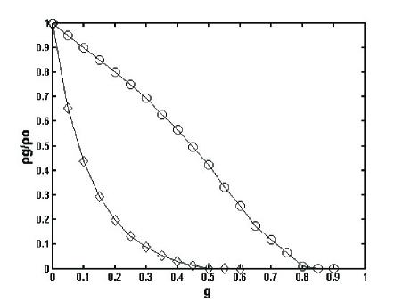
(a)

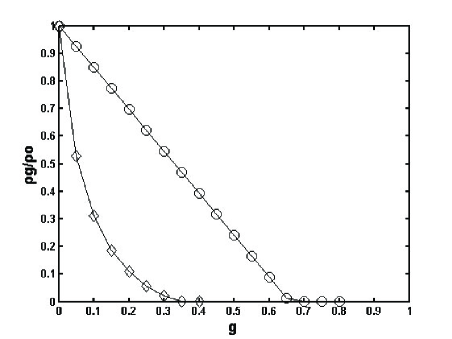
(b)

Figure 1: The relation of $\rho_{g}/\rho_{0}$ and density $g$ on the WS model with $N=10^{4}$, $\langle k\rangle=8$, $P=1$, $\lambda=0.25$ (a) circles represent the random immunization and diamonds represent the random “network monitors”, (b) circles represent the targeted immunization and diamonds represent the targeted “network monitors”.

3 Eradicating epidemics on SF networks

In this section, we focus on heterogeneous networks especially on SF networks (we do not consider degree correlations here). Firstly, we test whether the random “network monitors” is effective or not on SF networks. We write the mean-field rate equation as:

$$\frac{\mathrm{d}\rho_{k}(t)}{\mathrm{d}t}=\lambda(1-g)k(1-\rho_{k}(t))\Theta(t)-f(k,g)\rho_{k}(t)$$ (7)

Here, $g$ represents the density of “network monitors” and the function $f(k,g)$ can be written as $f(k,g)=$min$(1,k\\ \sum\limits_{k^{\prime}}k^{\prime}p(k^{\prime})g_{k^{\prime}}/\langle k\rangle)$, which is the probability that an infected node with k links connects with some “network monitor”. In addition, $\rho_{k}(t)$ represents the density of infected nodes that have degree $k$ and we define the quantity $\Theta(t)=\sum\limits_{k}kp_{k}\rho_{k}(t)/\sum\limits_{s}sp_{s}$ as the probability of the susceptible node pointing to an infected node at time $t$. In Eq. (7), we observe that if we can keep $f(k,g)\equiv 1$, then the random “network monitors” is most efficient. It is apparent that if above condition is fulfilled, the effect of random “network monitors” is equivalent to the effect of random immunization strategy in the SIS model. From Ref. 2 we know that this immunization strategy is not particularly effective on SF networks in the SIS model. As a consequence, random “network monitors” is also not effective on SF networks.

Next, we investigate whether the targeted “network monitors” is effective or not on SF networks. After applying the targeted “network monitors”, we obtain the following mean-field equation:

$$\frac{\mathrm{d}\rho_{k}(t)}{\mathrm{d}t}=\lambda k(1-\rho_{k}(t)-g_{k})\Theta(t)-f(k,g)\rho_{k}(t)$$ (8)

In Eq. (8), $g_{k}$ represents the density of “network monitors” with degree $k$ and the function $f(k,g)$ can be written as $f(k,g)=$min$(1,k\sum\limits_{k^{\prime}}k^{\prime}p(k^{\prime})g_{k^{\prime}}/\langle k\rangle)$. Here we assume that after applying the targeted “network monitors”, the probability that a node with $k$ links is healthy is $(1-\rho_{k}(t)-g_{k})$. In the stationary state ($\mathrm{d}\rho_{k}(t)/\mathrm{d}t=0$) we obtain Eq. (9) from Eq. (8):

$$\lambda k(1-\rho_{k}-g_{k})\Theta=f(k,g)\rho_{k}$$ (9)

From Eq. (9) we can get the solution of $\rho_{k}(t)$ in the stationary state: $\rho_{k}=((1-g_{k})\lambda k\Theta)/(f(k,g)+\lambda k\Theta)$. Now inserting this result into the definition of $\Theta$, we can obtain Eq. (10):

$$\Theta=\frac{1}{\langle k\rangle}\sum\limits_{k}kp(k)\frac{(1-g_{k})\lambda k\Theta}{f(k,g)+\lambda k\Theta}$$ (10)

Here, we define an auxiliary function

$$F(\Theta)=\frac{1}{\langle k\rangle}\sum\limits_{k}kp(k)\frac{(1-g_{k})\lambda k\Theta}{f(k,g)+\lambda k\Theta}-\Theta$$

It is apparent that $F(0)=0$. Since $\frac{1}{\langle k\rangle}\sum\limits_{k}kp(k)\frac{(1-g_{k})\lambda k\Theta}{f(k,g)+\lambda k\Theta}\leq\frac{1}{\langle k\rangle}\sum\limits_{k}kp(k)\frac{(1-g_{k})\lambda k\Theta}{\lambda k\Theta}<1$, we have $F(1)<0$. If $F^{\prime}(0)<0$, then $F(\Theta)<0$ for some $\Theta\in(0,1]$. But if $F^{\prime}(0)\geq 0$, there is a $\Theta_{1}\in(0,1)$ that satisfies $F(\Theta_{1})>0$. Then by the intermediate theorem, there is a $\Theta\in(\Theta_{1},1)$ satisfies $F(\Theta)=0$. Consequently, if there is a $\Theta\in(0,1)$ that satisfies $F(\Theta)=0$, $F^{\prime}(0)\geq 0$. It is equivalent to say that if there is a non-zero solution of Eq. (10), then:

$$\frac{\mathrm{d}}{\mathrm{d}\Theta}(\frac{1}{\langle k\rangle}\sum\limits_{k}kp(k)\frac{(1-g_{k})\lambda k\Theta}{f(k,g)+\lambda k\Theta})\mid_{\Theta=0}\geq 1$$ (11)

So we can get Eq. (12):

$$\frac{\lambda}{\langle k\rangle}\sum_{k}\frac{k^{2}(1-g_{k})p(k)}{f(k,g_{c})}=1$$ (12)

Here $g_{c}$ represents critical density of “network monitors”. We define a new quantity $k_{t}$. When $k>k_{t}$ the density of “network monitors” $g_{k}=1$ and when $k\leq k_{t}$ the density of “network monitors” $g_{k}=0$. So we rewrite Eq. (12) as follows:

$$\frac{\lambda}{\langle k\rangle}\sum\limits_{k=0}^{k_{t}}\frac{k^{2}p(k)}{f(k,g_{c})}=1$$ (13)

From the definition of $k_{t}$ we can get $g_{c}=\sum\limits_{k>k_{t}}p(k)\approx 1-\int\nolimits_{0}^{k_{t}}p(k)\mathrm{d}k$. Then we can obtain the expression of $k_{t}$ as a function of $g_{c}$. Finally, we insert this expression into Eq. (13) to get the critical density $g_{c}$.

In order to support our analysis, we perform numerical simulations on the BA network 17 with the network size $N=10^{4}$, $m_{0}=7$, $m=4$ and $\lambda=0.25$. Initially, we infect only one node.

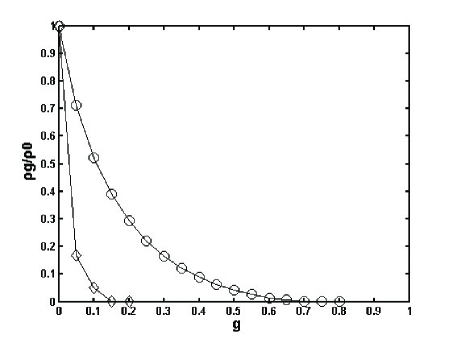
Figure 2: The relation of $\rho_{g}/\rho_{0}$ and density $g$ on the BA model with $N=10^{4}$, $m_{0}=7$, $m=4$, $\lambda=0.25$. Circles represent the strategy of random “network monitors” and diamonds represent the strategy of targeted “network monitors”.

Fig. 2 shows the relation between reduced density of infected nodes $\rho_{g}/\rho_{0}$ in the end and the density of “network monitors” $g$. In Fig. 2, circles represent the data of the random “network monitors”. We observe that the random “network monitors” is not particularly effective. We should immunize large proportion of nodes as monitors to eradicate infection. On the contrary, we find that the targeted “network monitors” is effective. This fact can be observed in Fig. 2, in which the critical density of “network monitors” $g_{c}\approx 0.15$.

4 Discussion and conclusions

The main conclusion can be summarized as follows:
  $1.$ If we can only install and update the antivirus programs with the fraction $\alpha$ ($0<\alpha<<1$) computer nodes on the network, the random immunization and the targeted immunization are not efficient to prevent computer viruses spreading on the homogeneous networks.
  $2.$ We introduce a policy to protect the computer networks, namely, “network monitors”. Specifically, we choose some computer nodes on the network as the “network monitors”. They play two roles. On the one hand, They are immune to computer viruses. On the other hand, “network monitors” can monitor their neighboring nodes’ behaviors. If they find their neighbors infected by computer viruses, they can eliminate computer viruses from infected neighbors. Based on different approach to select nodes as the “network monitors”, we divide the “network monitors” into two types, one is the random “network monitors” and the other is the targeted “network monitors”. Through analysis, we find that the random “network monitors” and the targeted “network monitors” are effective on WS networks. Besides, the targeted “network monitors” is effective on SF networks. Numerical simulations confirm our analysis.

In fact, our new strategy is similar with the contact tracing 18 but we explicitly set monitors on the network. If possible, we can initially install antivirus programs in each computer node on the network and then only update antivirus programs in “network monitors” . So the recovering probability of the infective computer node is generally not zero, since old version antivirus programs can “kill” ordinary viruses. Then the number of “network monitors” chosen to eradicate computer viruses is smaller than our analysis. It demonstrates that the strategy of the “network monitors” is practical and efficient that we need only update small fraction computers’ antivirus programs and fire walls so that the security of the whole computer network can be kept.

The author thanks Robert Ellis, Hemanshu Kaul and Michael Pelsmajer for meaningful comments.

References

- (1) D.H. Zanette and M. Kuperman, Physica A 309, 445 (2002)
- (2) R. Pastor-Satorras and A. Vespignani, Phys. Rev. E 65, 036104 (2002)
- (3) N. Madar, T. Kalisky, R. Cohen, D. ben-Avraham and S. Havlin, Eur. Phys. J. B 38, 269 (2004)
- (4) R. Cohen, S. Havlin and D. ben-Avraham, Phys. Rev. Lett. 91, 247901 (2003)
- (5) M.E.J. Newman, SIAM Rev. 45, 167 (2003)
- (6) M.E.J. Newman, Phys. Rev. E 66, 016128 (2002)
- (7) M.E.J. Newman, S.H. Strogatz and D.J. Watts, Phys. Rev. E 64, 026118 (2001)
- (8) C. Moore and M.E.J. Newman, Phys. Rev. E 61, 5678 (2000)
- (9) R. Albert, H. Jeong, and A.-L. Barabási, Nature (London) 406, 378 (2000).
- (10) D.S. Callaway, M.E.J. Newman, S.H. Strogatz, and D.J. Watts, Phys. Rev. Lett. 85, 5468 (2000)
- (11) R. Cohen, K. Erez, D. ben-Avraham and S. Havlin, Phys. Rev. Lett. 85, 4626 (2000)
- (12) R. Cohen, K. Erez, D. ben-Avraham and S. Havlin, Phys. Rev. Lett. 86, 3682 (2001)
- (13) D.J. Watts and S.H. Strogatz, Nature (London) 393, 440 (1998).
- (14) B. Bolloba s, Random Graphs (Academic Press, New York,1985).
- (15) M. Barthélemy, A. Barrat, R. Pastor-Satorras and A. Vespignani, Phys. Rev. Lett. 92, 178701 (2004)
- (16) R. Albert and A.-L. Barabási, Rev. Mod. Phys. 74, 47 (2002)
- (17) A.-L. Barabási and R. Albert, Science 286, 509 (1999)
- (18) R. Huerta and L.S. Tsimring, Phys. Rev. E 66, 056115 (2002)