Incremental Learning of 3D-DCT Compact Representations for Robust Visual Tracking

Abstract

Visual tracking usually requires an object appearance model that is robust to changing illumination, pose and other factors encountered in video. Many recent trackers utilize appearance samples in previous frames to form the bases upon which the object appearance model is built. This approach has the following limitations: (a) the bases are data driven, so they can be easily corrupted; and (b) it is difficult to robustly update the bases in challenging situations.

In this paper, we construct an appearance model using the 3D discrete cosine transform (3D-DCT). The 3D-DCT is based on a set of cosine basis functions, which are determined by the dimensions of the 3D signal and thus independent of the input video data. In addition, the 3D-DCT can generate a compact energy spectrum whose high-frequency coefficients are sparse if the appearance samples are similar. By discarding these high-frequency coefficients, we simultaneously obtain a compact 3D-DCT based object representation and a signal reconstruction-based similarity measure (reflecting the information loss from signal reconstruction). To efficiently update the object representation, we propose an incremental 3D-DCT algorithm, which decomposes the 3D-DCT into successive operations of the 2D discrete cosine transform (2D-DCT) and 1D discrete cosine transform (1D-DCT) on the input video data. As a result, the incremental 3D-DCT algorithm only needs to compute the 2D-DCT for newly added frames as well as the 1D-DCT along the third dimension, which significantly reduces the computational complexity. Based on this incremental 3D-DCT algorithm, we design a discriminative criterion to evaluate the likelihood of a test sample belonging to the foreground object. We then embed the discriminative criterion into a particle filtering framework for object state inference over time. Experimental results demonstrate the effectiveness and robustness of the proposed tracker.

I Introduction

Visual tracking of a moving object is a fundamental problem in computer vision. It has a wide range of applications including visual surveillance, human behavior analysis, motion event detection, and video retrieval. Despite much effort on this topic, it remains a challenging problem because of object appearance variations due to illumination changes, occlusions, pose changes, cluttered and moving backgrounds, etc. Thus, a crucial element of visual tracking is to use an effective object appearance model that is robust to such challenges.

Since it is difficult to explicitly model complex appearance changes, a popular approach is to learn a low-dimensional subspace (e.g., eigenspace [1, 2]), which accommodates the object’s observed appearance variations. This allows the appearance model to reflect the time-varying properties of object appearance during tracking (e.g., learning the appearance of the object from multiple observed poses). By computing the sample-to-subspace distance (e.g., reconstruction error [1, 2]), the approach can measure the information loss that results from projecting a test sample to the low-dimensional subspace. Using the information loss, the approach can evaluate the likelihood of a test sample belonging to the foreground object. Since the approach is data driven, it needs to compute the subspace basis vectors as well as the corresponding coefficients.

Inspired by the success of subspace learning for visual tracking, we propose an alternative object representation based on the 3D discrete cosine transform (3D-DCT), which has a set of fixed projection bases (i.e., cosine basis functions). Using these fixed projection bases, the proposed object representation only needs to compute the corresponding projection coefficients (3D-DCT coefficients). Compared with incremental principal component analysis [1], this leads to a much simpler computational process, which is more robust to many types of appearance change and enables fast implementation.

The DCT has a long history in the signal processing community as a tool for encoding images and video. It has been shown to have desirable properties for representing video, many of which also make it a promising object representation for visual tracking in video:

• As illustrated in Fig. 1, the DCT leads to a compact object representation with sparse transform coefficients if a signal is self-correlated in both spatial and temporal dimensions. This means that the reconstruction error induced by removing a subset of coefficients is typically small. Additionally, high-frequency image noise or rapid appearance changes are often isolated in a small number of coefficients;

• The DCT’s cosine basis functions are determined by the signal dimensions that are fixed at initialization. Thus, the DCT’s cosine basis functions are fixed throughout tracking, resulting in a simple procedure of constructing the DCT-based object representation;

• The DCT only requires single-level cosine decomposition to approximate the original signal, which again is computationally efficient and also lends itself to incremental calculation, which is useful for tracking.

Our idea is simply to represent a new sample by concatenating it with a collection of previous samples to form a 3D signal, and calculating its coefficients in the 3D-DCT space with some high-frequency components removed. Since the 3D-DCT encodes the temporal redundancy information of the 3D signal, the representation can capture the correlation between the new sample and the previous samples. Given a compression ratio (derived from discarding some high-frequency components), if the new sample can still be effectively reconstructed with a relatively low reconstruction error, then it is correlated with the previous samples and is likely to be an object sample. The fact that every sample is represented by using the same cosine basis functions makes it very easy to perform the likelihood evaluations of samples.

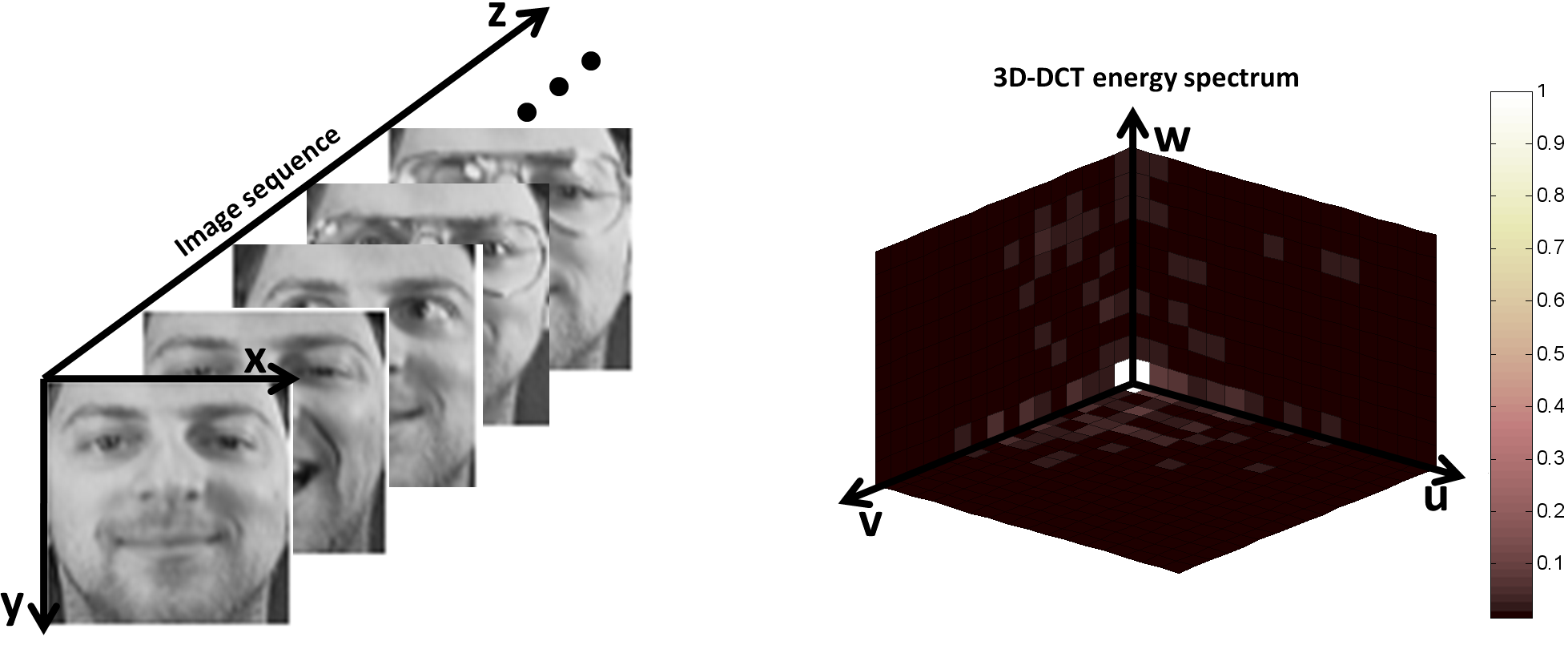
Figure 1: Illustration of 3D-DCT’s compactness. The left part shows a face image sequence, and the right part displays the corresponding energy spectrum of 3D-DCT. Clearly, it is seen from the right part that the energy spectrums of 3D-DCT are compact.

The DCT is not the only choice for compact representations using data-independent bases; others include Fourier and wavelet basis functions, which are also widely used in signal processing. The coefficients of these basis functions are capable of capturing the energy information at different frequencies. For example, both sine and cosine basis functions are adopted by the discrete Fourier transform (DFT) to generate the amplitude and phase frequency spectrums; wavelet basis functions (e.g., Haar and Gabor) aim to capture local detailed information (e.g., texture) of a signal at multiple resolutions by the wavelet transform (WT). Although we do not conduct experiments with these functions in this work, they can be used in our framework with only minor modification.

Using the 3D-DCT object representation, we propose a discriminative learning based tracker. The main contributions of this tracker are three-fold:

1. We utilize the signal compression power of the 3D-DCT to construct a novel representation of a tracked object. The representation retains the dense low-frequency 3D-DCT coefficients, and discards the relatively sparse high-frequency 3D-DCT coefficients. Based on this compact representation, the signal reconstruction error (measuring the information loss from signal reconstruction) is used to evaluate the likelihood of a test sample belonging to the foreground object given a set of training samples.

2. We propose an incremental 3D-DCT algorithm for efficiently updating the representation. The incremental algorithm decomposes 3D-DCT into the successive operations of the 2D-DCT and 1D-DCT on the input video data, and it only needs to compute the 2D-DCT for newly added frames (referred to in Equ. (18)) as well as the 1D-DCT along the third dimension, resulting in high computational efficiency. In particular, the cosine basis functions can be computed in advance, which significantly reduces the computational cost of the 3D-DCT.

3. We design a discriminative criterion (referred to in Equ. (20)) for predicting the confidence score of a test sample belonging to the foreground object. The discriminative criterion considers both the foreground and the background 3D-DCT reconstruction likelihoods, which enables the tracker to capture useful discriminative information for adapting to complicated appearance changes.

II Related work

Since our work focuses on learning compact object representations based on the 3D-DCT, we first discuss the DCT and its applications in relevant research fields. Then, we briefly review the related tracking algorithms using different types of object representations. As claimed in [3, 4], the DCT aims to use a set of mutually uncorrelated cosine basis functions to express a discrete signal in a linear manner. It has a wide range of applications in computer vision, pattern recognition, and multimedia, such as face recognition [5], image retrieval [6, 7], video object segmentation [8], video caption localization [9], etc. In these applications, the DCT is typically used for feature extraction, and aims to construct a compact DCT coefficient-based image representation that is robust to complicated factors (e.g., facial geometry and illumination changes). In this paper, we focus on how to construct an effective DCT-based object representation for robust visual tracking.

In the field of visual tracking, researchers have designed a variety of object representations, which can be roughly classified into two categories: generative object representations and discriminative object representations.

Recently, much work has been done in constructing generative object representations, including the integral histogram [10], kernel density estimation [11], mixture models [12, 13], subspace learning [1, 14], linear representation [15, 16, 17, 18, 19], visual tracking decomposition [20], covariance tracking [21, 2, 22], and so on. Some representative tracking algorithms based on generative object representations are reviewed as follows. Jepson et al. [13] design a more elaborate mixture model with an online EM algorithm to explicitly model appearance changes during tracking. Wang et al. [12] present an adaptive appearance model based on the Gaussian mixture model in a joint spatial-color space. Comaniciu et al. [23] propose a kernel-based tracking algorithm using the mean shift-based mode seeking procedure. Following the work of [23], some variants of the kernel-based tracking algorithm are proposed, e.g., [11, 24, 25]. Ross et al. [1] propose a generalized tracking framework based on the incremental PCA (principal component analysis) subspace learning method with a sample mean update. A sparse approximation based tracking algorithm using $\ell_{1}$-regularized minimization is proposed by Mei and Ling [15]. To achieve a real-time performance, Li et al. [18] present a compressive sensing $\ell_{1}$ tracker using an orthogonal matching pursuit algorithm, which is up to 6000 times faster than [15].

In contrast, another type of tracking algorithms try to construct a variety of discriminative object representations, which aim to maximize the inter-class separability between the object and non-object regions using discriminative learning techniques, including SVMs [26, 27, 28, 29], boosting [30, 31], discriminative feature selection [32], random forest [33], multiple instance learning [34], spatial attention learning [35], discriminative metric learning [36, 37], data-driven adaptation [38], etc. Some popular tracking algorithms based on discriminative object representations are described as follows. Grabner et al. [30] design an online AdaBoost classifier for discriminative feature selection during tracking, resulting in the robustness to the appearance variations caused by out-of-plane rotations and illumination changes. To alleviate the model drifting problem with [30], Grabner et al. [31] present a semi-supervised online boosting algorithm for tracking. Liu and Yu [39] present a gradient-based feature selection mechanism for online boosting learning, leading to the higher tracking efficiency. Avidan [40] builds an ensemble of online learned weak classifiers for pixel-wise classification, and then employ mean shift for object localization. Instead of using single-instance boosting, Babenko et al. [34] present a tracking system based on online multiple instance boosting, where an object is represented as a set of image patches. Besides, SVM-based object representations have also attracted much attention in recent years. Based on off-line SVM learning, Avidan [26] proposes a tracking algorithm for distinguishing a target vehicle from backgrounds. Later, Tian et al. [27] present a tracking system based on an ensemble of linear SVM classifiers, which can be adaptively weighted according to their discriminative abilities during different periods. Instead of using supervised learning, Tang et al. [28] present an online semi-supervised learning based tracker, which constructs two feature-specific SVM classifiers in a co-training framework.

As our tracking algorithm is based on the DCT, we give a brief review of the discrete cosine transform and its three basic versions for 1D, 2D, and 3D signals in the next section.

III The 3D-DCT for object representation

We first give an introduction to the 3D-DCT in Section III-A. Then, we derive and formulate the DCT’s matrix forms (used for object representation) in Section III-B. Next, we address the problem of how to use the 3D-DCT as a compact object representation in Section III-C. Finally, we propose an incremental 3D-DCT algorithm to efficiently compute the 3D-DCT in Section III-D.

III-A 3D-DCT definitions and notations

The goal of the discrete cosine transform (DCT) is to express a discrete signal, such as a digital image or video, as a linear combination of mutually uncorrelated cosine basis functions (CBFs), each of which encodes frequency-specific information of the discrete signal.

We briefly define the 1D-DCT, 2D-DCT, and 3D-DCT, which are applied to 1D signal $\left(f_{\mathbf{I}}(x)\right)_{x=0}^{N_{1}-1}$, 2D signal $\left(f_{\mathbf{II}}(x,y)\right)_{N_{1}\times N_{2}}$ and 3D signal $\left(f_{\mathbf{III}}(x,y,z)\right)_{N_{1}\times N_{2}\times N_{3}}$ respectively:

$$C_{\mathbf{I}}(u)=\alpha_{1}(u)\sum_{x=0}^{N_{1}-1}f_{\mathbf{I}}(x)\cos\left[\frac{\pi(2x+1)u}{2N_{1}}\right],$$ (1)

$$C_{\mathbf{II}}(u,v)=\alpha_{1}(u)\alpha_{2}(v)\sum_{x=0}^{N_{1}-1}\sum_{y=0}^{N_{2}-1}f_{\mathbf{II}}(x,y)\cos\left[\frac{\pi(2x+1)u}{2N_{1}}\right]\cos\left[\frac{\pi(2y+1)v}{2N_{2}}\right],$$ (2)

$$\begin{array}[]{l}C_{\mathbf{III}}(u,v,w)=\alpha_{1}(u)\alpha_{2}(v)\alpha_{3}(w)\sum_{x=0}^{N_{1}-1}\sum_{y=0}^{N_{2}-1}\sum_{z=0}^{N_{3}-1}f_{\mathbf{III}}(x,y,z)\\ \hskip 88.2037pt\cdot\left\{\cos\left[\frac{\pi(2x+1)u}{2N_{1}}\right]\cos\left[\frac{\pi(2y+1)v}{2N_{2}}\right]\cos\left[\frac{\pi(2z+1)w}{2N_{3}}\right]\right\},\end{array}$$ (3)

where $u\in\{0,1,\ldots,N_{1}-1\}$, $v\in\{0,1,\ldots,N_{2}-1\}$, $w\in\{0,1,\ldots,N_{3}-1\}$ and $\alpha_{k}(u)$ is defined as

$$\alpha_{k}(u)=\left\{\begin{array}[]{ll}\sqrt{\frac{1}{N_{k}}},&\mbox{if}\thickspace u=0;\\ \sqrt{\frac{2}{N_{k}}},&\mbox{otherwise};\end{array}\right.$$ (4)

where $k$ is a positive integer.

The corresponding inverse DCTs (referred to as 1D-IDCT, 2D-IDCT, and 3D-IDCT) are defined as:

$$f_{\mathbf{I}}(x)=\sum_{u=0}^{N_{1}-1}C_{\mathbf{I}}(u)\underbrace{\alpha_{1}(u)\cos\left[\frac{\pi(2x+1)u}{2N_{1}}\right]}_{\mbox{1D-DCT CBF}},$$ (5)

$$f_{\mathbf{II}}(x,y)=\sum_{u=0}^{N_{1}-1}\sum_{v=0}^{N_{2}-1}C_{\mathbf{II}}(u,v)\underbrace{\alpha_{1}(u)\alpha_{2}(v)\cos\left[\frac{\pi(2x+1)u}{2N_{1}}\right]\cos\left[\frac{\pi(2y+1)v}{2N_{2}}\right]}_{\mbox{2D-DCT CBF}},$$ (6)

$$\begin{array}[]{l}f_{\mathbf{III}}(x,y,z)=\sum_{w=0}^{N_{3}-1}\sum_{u=0}^{N_{1}-1}\sum_{v=0}^{N_{2}-1}C_{\mathbf{III}}(u,v,w)\cdot\\ \underbrace{\alpha_{1}(u)\alpha_{2}(v)\alpha_{3}(w)\cos\left[\frac{\pi(2x+1)u}{2N_{1}}\right]\cos\left[\frac{\pi(2y+1)v}{2N_{2}}\right]\cos\left[\frac{\pi(2z+1)w}{2N_{3}}\right]}_{\mbox{3D-DCT CBF}}.\end{array}$$ (7)

The low-frequency CBFs reflect the larger-scale energy information (e.g., mean value) of the discrete signal, while the high-frequency CBFs capture the smaller-scale energy information (e.g., texture) of the discrete signal. Based on these CBFs, the original discrete signal can be transformed into a DCT coefficient space whose dimensions are mutually uncorrelated. Furthermore, the output of the DCT is typically sparse, which is useful for signal compression and also for tracking, as will be shown in the following sections.

III-B 3D-DCT matrix formulation

Let $\mathbf{C}_{\mathbf{I}}=\left(C_{\mathbf{I}}(0),C_{\mathbf{I}}(1),\ldots,C_{\mathbf{I}}(N_{1}-1)\right)^{T}$ denote the 1D-DCT coefficient column vector. Based on Equ. (1), $\mathbf{C}_{\mathbf{I}}$ can be rewritten in a matrix form: $\mathbf{C}_{\mathbf{I}}=\mathbf{A}_{1}\mathbf{f}$, where $\mathbf{f}$ is a column vector: $\mathbf{f}=(f_{\mathbf{I}}(0),f_{\mathbf{I}}(1),\ldots,f_{\mathbf{I}}(N_{1}-1))^{T}$ and $\mathbf{A}_{1}=\left(a_{1}(u,x)\right)_{N_{1}\times N_{1}}$ is a cosine basis matrix whose entries are given by:

$$a_{1}(u,x)=\alpha_{1}(u)\cos\left[\frac{\pi(2x+1)u}{2N_{1}}\right].$$ (8)

The matrix form of 1D-IDCT can be written as: $\mathbf{f}=\mathbf{A}_{1}^{-1}\mathbf{C}_{\mathbf{I}}$. Since $\mathbf{A}_{1}$ is an orthonormal matrix, $\mathbf{f}=\mathbf{A}_{1}^{T}\mathbf{C}_{\mathbf{I}}$.

The 2D-DCT coefficient matrix $\mathbf{C}_{\mathbf{II}}=(C_{\mathbf{II}}(u,v))_{N_{1}\times N_{2}}$ corresponding to Equ. (2) is formulated as: $\mathbf{C}_{\mathbf{II}}=\mathbf{A}_{1}\mathbf{F}\mathbf{A}_{2}^{T}$, where $\mathbf{F}=(f_{\mathbf{II}}(x,y))_{N_{1}\times N_{2}}$ is the original 2D signal, $\mathbf{A}_{1}$ is defined in Equ. (8), and $\mathbf{A}_{2}$ is defined as $(a_{2}(v,y))_{N_{2}\times N_{2}}$ such that

$$a_{2}(v,y)=\alpha_{2}(v)\cos\left[\frac{\pi(2y+1)v}{2N_{2}}\right].$$ (9)

The matrix form of the 2D-IDCT can be expressed as: $\mathbf{F}=\mathbf{A}_{1}^{-1}\mathbf{C}_{\mathbf{II}}(\mathbf{A}_{2}^{T})^{-1}$. Since the DCT basis functions are orthonormal, we have $\mathbf{F}=\mathbf{A}_{1}^{T}\mathbf{C}_{\mathbf{II}}\mathbf{A}_{2}$.

Similarly, the 3D-DCT can be decomposed into a succession of the 2D-DCT and 1D-DCT operations. Let $\mathcal{F}=(f_{\mathbf{III}}(x,y,z))_{N_{1}\times N_{2}\times N_{3}}$ denote a 3D signal. Mathematically, $\mathcal{F}$ can be viewed as a three-order tensor, i.e., $\mathcal{F}\in\mathcal{R}^{N_{1}\times N_{2}\times N_{3}}$. Consequently, we need to introduce terminology for the mode-$m$ product defined in tensor algebra [41]. Let $\mathcal{B}\in\mathcal{R}^{I_{1}\times I_{2}\times\ldots\times I_{M}}$ denote an $M$-order tensor, each element of which is represented as $b(i_{1},\ldots,i_{m}\ldots,i_{M})$ with $1\leq i_{m}\leq I_{m}$. In tensor terminology, each dimension of a tensor is associated with a “mode”. The mode-$m$ product of the tensor $\mathcal{B}$ by a matrix $\mathbf{\Phi}=(\phi(j_{m},i_{m}))_{J_{m}\times I_{m}}$ is denoted as $\mathcal{B}\times_{m}\mathbf{\Phi}$ whose entries are as follows:

$$\left(\mathcal{B}\times_{m}\mathbf{\Phi}\right)(i_{1},\ldots,i_{m-1},j_{m},i_{m+1},\ldots,i_{M})=\sum_{i_{m}}b(i_{1},\ldots,i_{m},\ldots,i_{M})\phi(j_{m},i_{m}),$$ (10)

where $\times_{m}$ is the mode-$m$ product operator and $1\leq m\leq M$. Given two matrices $\mathbf{G}\in\mathcal{R}^{J_{m}\times I_{m}}$ and $\mathbf{H}\in\mathcal{R}^{J_{n}\times I_{n}}$ such that $m\neq n$, the following relation holds:

$$(\mathcal{B}\times_{m}\mathbf{G})\times_{n}\mathbf{H}=(\mathcal{B}\times_{n}\mathbf{H})\times_{m}\mathbf{G}=\mathcal{B}\times_{m}\mathbf{G}\times_{n}\mathbf{H}.$$ (11)

Based on the above tensor algebra, the 3D-DCT coefficient matrix $\mathbf{C}_{\mathbf{III}}=(C_{\mathbf{III}}(u,v,w))_{N_{1}\times N_{2}\times N_{3}}$ can be formulated as: $\mathbf{C}_{\mathbf{III}}=\mathcal{F}\times_{1}\mathbf{A}_{1}\times_{2}\mathbf{A}_{2}\times_{3}\mathbf{A}_{3}$, where $\mathbf{A}_{3}=(a_{3}(w,z))_{N_{3}\times N_{3}}$ has a similar definition to $\mathbf{A}_{1}$ and $\mathbf{A}_{2}$:

$$a_{3}(w,z)=\alpha_{3}(w)\cos\left[\frac{\pi(2z+1)w}{2N_{3}}\right].$$ (12)

Accordingly, 3D-IDCT is formulated as: $\mathcal{F}=\mathbf{C}_{\mathbf{III}}\times_{1}\mathbf{A}_{1}^{-1}\times_{2}\mathbf{A}^{-1}_{2}\times_{3}\mathbf{A}^{-1}_{3}$. Since $\mathbf{A}_{k}(1\leq k\leq 3)$ is an orthonormal matrix, $\mathcal{F}$ can be rewritten as:

$$\mathcal{F}=\mathbf{C}_{\mathbf{III}}\times_{1}\mathbf{A}_{1}^{T}\times_{2}\mathbf{A}^{T}_{2}\times_{3}\mathbf{A}^{T}_{3}.$$ (13)

In fact, the 1D-DCT and 2D-DCT are two special cases of the 3D-DCT because 1D vectors and 2D matrices are 1-order and 2-order tensors, respectively, namely, $\mathbf{f}\times_{1}\mathbf{A}_{1}=\mathbf{A}_{1}\mathbf{f}$ and $\mathbf{F}\times_{1}\mathbf{A}_{1}\times_{2}\mathbf{A}_{2}=\mathbf{A}_{1}\mathbf{F}\mathbf{A}_{2}^{T}$.

III-C Compact object representation using the 3D-DCT

For visual tracking, an input video sequence can be viewed as 3D data, so the 3D-DCT is a natural choice for object representation. Given a sequence of normalized object image regions $\mathcal{F}=\left(f_{\mathbf{III}}(x,y,z)\right)_{N_{1}\times N_{2}\times N_{3}}$ from previous frames and a candidate image region $\left(\tau(x,y)\right)_{N_{1}\times N_{2}}$ in the current frame, we have a new image sequence $\mathcal{F}^{{}^{\prime}}=\left(f_{\mathbf{III}}(x,y,z)\right)_{N_{1}\times N_{2}\times(N_{3}+1)}$ where the first $N_{3}$ images correspond to $\mathcal{F}$ and the last image (i.e., the $(N_{3}+1)$th image) is $\left(\tau(x,y)\right)_{N_{1}\times N_{2}}$. According to Equ. (13), $\mathcal{F}^{{}^{\prime}}$ can be expressed as:

$$\mathcal{F}^{{}^{\prime}}=\mathbf{C}^{{}^{\prime}}_{\mathbf{III}}\times_{1}\mathbf{A}_{1}^{T}\times_{2}\mathbf{A}^{T}_{2}\times_{3}(\mathbf{A}^{{}^{\prime}}_{3})^{T},$$ (14)

where $\mathbf{C}^{{}^{\prime}}_{\mathbf{III}}\in\mathcal{R}^{N_{1}\times N_{2}\times(N_{3}+1)}$ is the 3D-DCT coefficient matrix: $\mathbf{C}^{{}^{\prime}}_{\mathbf{III}}=\mathcal{F}^{{}^{\prime}}\times_{1}\mathbf{A}_{1}\times_{2}\mathbf{A}_{2}\times_{3}\mathbf{A}^{{}^{\prime}}_{3}$ and $\mathbf{A}^{{}^{\prime}}_{3}\in\mathcal{R}^{(N_{3}+1)\times(N_{3}+1)}$ is a cosine basis matrix whose entry is defined as:

$$a^{{}^{\prime}}_{3}(w,z)=\left\{\begin{array}[]{ll}\sqrt{\frac{1}{N_{3}+1}},&\mbox{if}\thickspace w=0;\\ \sqrt{\frac{2}{N_{3}+1}}\cos\left[\frac{\pi(2z+1)w}{2(N_{3}+1)}\right],&\mbox{otherwise}.\end{array}\right.$$ (15)

According to the properties of the 3D-DCT, the larger the values of $(u,v,w)$ are, the higher frequency the corresponding elements of $\mathbf{C}^{{}^{\prime}}_{\mathbf{III}}$ encode. Usually, the high-frequency coefficients are sparse while the low-frequency coefficients are relatively dense. Recently, PCA (principal component analysis) tracking [1] builds a compact subspace model which maintains a set of principal eigenvectors controlling the degree of structural information preservation. Inspired by PCA tracking [1], we compress the 3D-DCT object representation by retaining the relatively low-frequency elements of $\mathbf{C}^{{}^{\prime}}_{\mathbf{III}}$ around the origin, i.e., $\{(u,v,w)|u\leq\delta_{u},v\leq\delta_{v},w\leq\delta_{w}\}$. As a result, we can obtain a compact 3D-DCT coefficient matrix $C^{\ast}_{\mathbf{III}}$. Then, $\mathcal{F}^{{}^{\prime}}$ can be approximated by:

$$\mathcal{F}^{{}^{\prime}}\approx\mathcal{F}^{\ast}=\mathbf{C}^{\ast}_{\mathbf{III}}\times_{1}\mathbf{A}_{1}^{T}\times_{2}\mathbf{A}^{T}_{2}\times_{3}(\mathbf{A}^{{}^{\prime}}_{3})^{T}.$$ (16)

Let $\mathcal{F}^{\ast}=\left(f^{\ast}_{\mathbf{III}}(x,y,z)\right)_{N_{1}\times N_{2}\times(N_{3}+1)}$ denote the corresponding reconstructed image sequence of $\mathcal{F}^{{}^{\prime}}$. The loss of high frequency components introduces a reconstruction error $\|\tau-f^{\ast}_{\mathbf{III}}(:,:,N_{3}+1)\|$, which forms the basis of the likelihood measure, as shown in Section IV-B.

Input: • Cosine basis matrices $\mathbf{A}_{1}$ and $\mathbf{A}_{2}$ (whose values are fixed given $N_{1}$ and $N_{2}$) • Cosine basis matrices $\mathbf{A}^{{}^{\prime}}_{3}$ • New image $\left(\tau(x,y)\right)_{N_{1}\times N_{2}}$ • $\mathbf{D}=\mathcal{F}\times_{1}\mathbf{A}_{1}\times_{2}\mathbf{A}_{2}$ of the previous image sequence $\mathcal{F}=\left(f_{\mathbf{III}}(x,y,z)\right)_{N_{1}\times N_{2}\times N_{3}}$

begin

      

1. Use the FFT to efficiently compute the 2D-DCT of $\tau$;

2. Update $\mathbf{D}^{{}^{\prime}}$ according to Equ. (18);

3. Employ the FFT to efficiently obtain the 1D-DCT of $\mathbf{D}^{{}^{\prime}}$ along the third dimension.

Output:

• 3D-DCT (i.e., $\mathbf{C}^{{}^{\prime}}_{\mathbf{III}}$) of the current image sequence $\mathcal{F}^{{}^{\prime}}=\left(f_{\mathbf{III}}(x,y,z)\right)_{N_{1}\times N_{2}\times(N_{3}+1)}$

Algorithm 1 Incremental 3D-DCT for object representation.

III-D Incremental 3D-DCT

Given a sequence of training images, we have shown how to use the 3D-DCT to represent an object for visual tracking, in Equ. (16). As the object’s appearance changes with time, it is also necessary to update the object representation. Consequently, we propose an incremental 3D-DCT algorithm which can efficiently update the 3D-DCT based object representation as new data arrive.

Given a new image $\left(\tau(x,y)\right)_{N_{1}\times N_{2}}$ and the transform coefficient matrix $\mathbf{D}=\mathcal{F}\times_{1}\mathbf{A}_{1}\times_{2}\mathbf{A}_{2}\in\mathcal{R}^{{N_{1}\times N_{2}\times N_{3}}}$ of previous images $\mathcal{F}=\left(f_{\mathbf{III}}(x,y,z)\right)_{N_{1}\times N_{2}\times N_{3}}$, the incremental 3D-DCT algorithm aims to efficiently compute the 3D-DCT coefficient matrix $\mathbf{C}^{{}^{\prime}}_{\mathbf{III}}\in\mathcal{R}^{{N_{1}\times N_{2}\times(N_{3}+1)}}$ of the previous images with the current image appended: $\mathcal{F}^{{}^{\prime}}=\left(f_{\mathbf{III}}(x,y,z)\right)_{N_{1}\times N_{2}\times(N_{3}+1)}$ with the last image being $\left(\tau(x,y)\right)_{N_{1}\times N_{2}}$. Mathematically, $\mathbf{C}^{{}^{\prime}}_{\mathbf{III}}$ is formulated as:

$$\mathbf{C}^{{}^{\prime}}_{\mathbf{III}}=\mathcal{F}^{{}^{\prime}}\times_{1}\mathbf{A}_{1}\times_{2}\mathbf{A}_{2}\times_{3}\mathbf{A}^{{}^{\prime}}_{3},$$ (17)

where $\mathbf{A}^{{}^{\prime}}_{3}\in\mathcal{R}^{(N_{3}+1)\times(N_{3}+1)}$ is referred to in Equ. (14). In principle, Equ. (17) can be computed in the following two stages: 1) compute the 2D-DCT coefficients for each image, i.e., $\mathbf{D}^{{}^{\prime}}=\mathcal{F}^{{}^{\prime}}\times_{1}\mathbf{A}_{1}\times_{2}\mathbf{A}_{2}$; and 2) calculate the 1D-DCT coefficients along the time dimension, i.e, $\mathbf{C}^{{}^{\prime}}_{\mathbf{III}}=\mathbf{D}^{{}^{\prime}}\times_{3}\mathbf{A}^{{}^{\prime}}_{3}$.

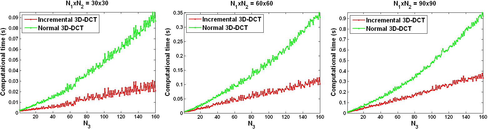
Figure 2: Comparison on the computational time between the normal 3D-DCT and our incremental 3D-DCT. The three subfigures correspond to different configurations of $N_{1}\times N_{2}$ (i.e., $30\times 30$, $60\times 60$, and $90\times 90$). In each subfigure, the x-axis is associated with $N_{3}$; the y-axis corresponds to the computational time. Clearly, as $N_{3}$ increases, the computational time of the normal 3D-DCT grows much faster than that of the incremental 3D-DCT.

According to the definition of the 3D-DCT, the CBF matrices $\mathbf{A}_{1}$ and $\mathbf{A}_{2}$ only depend on the row and column dimensions (i.e., $N_{1}$ and $N_{2}$), respectively. Since both $N_{1}$ and $N_{2}$ are unchanged during visual tracking, both $\mathbf{A}_{1}$ and $\mathbf{A}_{2}$ remain constant. In addition, $\mathcal{F}^{{}^{\prime}}$ is a concatenation of $\mathcal{F}$ and $\left(\tau(x,y)\right)_{N_{1}\times N_{2}}$ along the third dimension. According to the property of tensor algebra, $\mathbf{D}^{{}^{\prime}}$ can be decomposed as:

$$\mathbf{D}^{{}^{\prime}}(:,:,k)=\left\{\begin{array}[]{ll}\mathbf{D}(:,:,k),&\mbox{if}\thickspace 1\leq k\leq N_{3};\\ \tau\times_{1}\mathbf{A}_{1}\times_{2}\mathbf{A}_{2},&k=N_{3}+1;\end{array}\right.$$ (18)

Given $\mathbf{D}$, $\mathbf{D}^{\prime}$ can be efficiently updated by only computing the term $\tau\times_{1}\mathbf{A}_{1}\times_{2}\mathbf{A}_{2}$. Moreover, $\mathbf{A}^{{}^{\prime}}_{3}$ is only dependent on the variable $N_{3}$. Once $N_{3}$ is fixed, $\mathbf{A}^{{}^{\prime}}_{3}$ is also fixed. In addition, $\tau\times_{1}\mathbf{A}_{1}\times_{2}\mathbf{A}_{2}$ can be viewed as the 2D-DCT along the first two dimensions (i.e., $x$ and $y$); and $\mathbf{C}^{{}^{\prime}}_{\mathbf{III}}=\mathbf{D}^{{}^{\prime}}\times_{3}\mathbf{A}^{{}^{\prime}}_{3}$ can be viewed as the 1D-DCT along the time dimension. To further reduce the computational time of the 1D-DCT and 2D-DCT, we employ a fast algorithm using the Fast Fourier Transform (FFT) to efficiently compute the DCT and its inverse [3, 4]. The complete procedure of the incremental 3D-DCT algorithm is summarized in Algorithm 1.

The complexity of our incremental algorithm is $O(N_{1}N_{2}(\log N_{1}+\log N_{2})+N_{1}N_{2}N_{3}\log N_{3})$ at each frame. In contrast, using a traditional batch-mode strategy for DCT computation, the complexity of the normal 3D-DCT algorithm becomes $O(N_{1}N_{2}N_{3}(\log N_{1}+\log N_{2}+\log N_{3}))$. To illustrate the computational efficiency of the incremental 3D-DCT algorithm, Fig. 2 shows the computational time of the incremental 3D-DCT and normal 3D-DCT algorithms for different values of $N_{1}$, $N_{2}$, and $N_{3}$. Although the computation time of both algorithms increases with $N_{3}$, the growth rate of the incremental 3D-DCT algorithm is much lower.

Input: New frame $t$, previous object state $\mathbf{Z}_{t-1}^{\ast}$, previous positive and negative sample sets: $\mathcal{F}_{+}=\left(f^{+}_{\mathbf{III}}(x,y,z)\right)_{N_{1}\times N_{2}\times N^{+}_{3}}$ and $\mathcal{F}_{-}=\left(f^{-}_{\mathbf{III}}(x,y,z)\right)_{N_{1}\times N_{2}\times N^{-}_{3}}$, maximum buffer size $\mathbb{T}$.

Initialization:

– $t=1$.

– Manually set the initial object state $\mathbf{Z}_{t}^{\ast}$.

– Collect positive (or negative) samples to form training sets $\mathcal{F}_{+}=\mathbb{Z}^{+}_{t}$ and $\mathcal{F}_{-}=\mathbb{Z}^{-}_{t}$ (see Section IV-A).

begin

• Sample $V$ candidate object states $\{\mathbf{Z}_{tj}\}_{j=1}^{V}$ according to Equ. (21).

• Crop out the corresponding image regions $\{o_{tj}\}_{j=1}^{V}$ of $\{\mathbf{Z}_{tj}\}_{j=1}^{V}$.

• Resize each candidate image region $o_{tj}$ to $N_{1}\times N_{2}$ pixels.

•  

  for each $\mathbf{Z}_{tj}$ do

1.        

   Find the $K$ nearest neighbors $\mathcal{F}_{+}^{K}\in\mathcal{R}^{N_{1}\times N_{2}\times K}$ (or $\mathcal{F}_{-}^{K}\in\mathcal{R}^{N_{1}\times N_{2}\times K}$) of a candidate

sample $\tau$ (i.e., $\tau=o_{tj}$) from $\mathcal{F}_{+}$ (or $\mathcal{F}_{-}$).

Obtain the 3D signals $\mathcal{F}_{+}^{{}^{\prime}}$ and $\mathcal{F}_{-}^{{}^{\prime}}$ through the concatenations of $(\mathcal{F}_{+}^{K},\tau)$ and $(\mathcal{F}_{-}^{K},\tau)$. 3. Perform the incremental 3D-DCT in Algorithm 1 to compute the 3D-DCT coefficient matrices: $\mathbf{C}^{{}^{\prime}}_{\mathbf{III}_{+}}$ and $\mathbf{C}^{{}^{\prime}}_{\mathbf{III}_{-}}$. 4.         Compute the compact 3D-DCT coefficient matrices $\mathbf{C}^{\ast}_{\mathbf{III}_{+}}$ and $\mathbf{C}^{\ast}_{\mathbf{III}_{-}}$ by discarding the high-frequency coefficients of

$\mathbf{C}^{{}^{\prime}}_{\mathbf{III}_{+}}$ and $\mathbf{C}^{{}^{\prime}}_{\mathbf{III}_{-}}$.

Calculate the reconstructed representations of $\mathcal{F}_{+}^{{}^{\prime}}$ and $\mathcal{F}_{-}^{{}^{\prime}}$ as $\mathcal{F}^{\ast}_{+}$ and $\mathcal{F}^{\ast}_{-}$ by Equ. (16). 6. Compute the reconstruction likelihoods $\mathcal{L}_{\tau_{+}}$ and $\mathcal{L}_{\tau_{-}}$ using Equ. (19). 7.         Calculate the final likelihood $\mathcal{L}^{\ast}_{\tau}$ using Equ. (20).

Determine the optimal object state $\mathbf{Z}_{t}^{\ast}$ by the MAP estimation (referred to in Equ. (22)). • Select positive (or negative) samples $\mathbb{Z}^{+}_{t}$ (or $\mathbb{Z}^{-}_{t}$) (referred to in Sec. IV-A). • Update the training sample sets $\mathcal{F}_{+}$ and $\mathcal{F}_{-}$ with $\mathcal{F}_{+}\bigcup\mathbb{Z}^{+}_{t}$ and $\mathcal{F}_{-}\bigcup\mathbb{Z}^{-}_{t}$. •   $N^{+}_{3}=N^{+}_{3}+|\mathbb{Z}^{+}_{t}|$ and $N^{-}_{3}=N^{-}_{3}+|\mathbb{Z}^{-}_{t}|$. • Maintain the positive and negative sample sets as follows: – If $N^{+}_{3}>\mathbb{T}$, then $\mathcal{F}_{+}$ is truncated to keep the last $\mathbb{T}$ elements. – If $N^{-}_{3}>\mathbb{T}$, then $\mathcal{F}_{-}$ is truncated to keep the last $\mathbb{T}$ elements.

Output: Current object state $\mathbf{Z}_{t}^{\ast}$, updated positive and negative sample sets $\mathcal{F}_{+}$ and $\mathcal{F}_{-}$.

Algorithm 2 Incremental 3D-DCT object tracking.

IV Incremental 3D-DCT based tracking

In this section, we propose a complete 3D-DCT based tracking algorithm, which is composed of three main modules:

• training sample selection: select positive and negative samples for discriminative learning;

• likelihood evaluation: compute the similarity between candidate samples and the 3D-DCT based observation model;

• motion estimation: generate candidate samples and estimate the object state.

Algorithm 2 lists the workflow of the proposed tracking algorithm. Next, we will discuss the three modules in detail.

IV-A Training sample selection

Similar to [34], we take a spatial distance-based strategy for training sample selection. Namely, the image regions from a small neighborhood around the object location are selected as positive samples, while the negative samples are generated by selecting the image regions which are relatively far from the object location. Specifically, we draw a number of samples $\mathbb{Z}_{t}$ from Equ. (21), and then an ascending sort for the samples from $\mathbb{Z}_{t}$ is made according to their spatial distances to the current object location, resulting in a sorted sample set $\mathbb{Z}_{t}^{s}$. By selecting the first few samples from $\mathbb{Z}_{t}^{s}$, we have a subset $\mathbb{Z}^{+}_{t}$ that is the final positive sample set, as shown in the middle part of Fig. 3. The negative sample set $\mathbb{Z}^{-}_{t}$ is generated in the area around the current tracker location, as shown in the right part of Fig. 3.

IV-B Likelihood evaluation

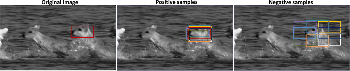
Figure 3: Illustration of training sample selection. The left subfigure plots the bounding box corresponding to the current tracker location; the middle subfigure shows the selected positive samples; and the right subfigure displays the selected negative samples. Different colors are assoicated with different samples.

During tracking, each of positive and negative samples is normalized to $N_{1}\times N_{2}$ pixels. Without loss of generality, we assume the numbers of the positive and negative samples to be $N^{+}_{3}$ and $N^{-}_{3}$. The positive and negative sample sequences are denoted as $\mathcal{F}_{+}=\left(f^{+}_{\mathbf{III}}(x,y,z)\right)_{N_{1}\times N_{2}\times N^{+}_{3}}$ and $\mathcal{F}_{-}=\left(f^{-}_{\mathbf{III}}(x,y,z)\right)_{N_{1}\times N_{2}\times N^{-}_{3}}$, respectively. Based on $\mathcal{F}_{+}$ and $\mathcal{F}_{-}$, we evaluate the likelihood of a candidate sample $\left(\tau(x,y)\right)_{N_{1}\times N_{2}}$ belonging to the foreground object. Since the appearance of $\mathcal{F}_{+}$ and $\mathcal{F}_{-}$ is likely to vary significantly as time progresses, it is not necessary for the 3D-DCT to use all samples in $\mathcal{F}_{+}$ and $\mathcal{F}_{-}$ to represent the candidate sample $\left(\tau(x,y)\right)_{N_{1}\times N_{2}}$. As pointed out by [42], locality is more essential than sparsity because locality usually results in sparsity but not necessarily vice versa. As a result, a locality-constrained strategy is taken to construct a compact object representation using the proposed incremental 3D-DCT algorithm.

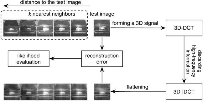
Figure 4: Illustration of the process of computing the reconstruction likelihood between test images and training images using the 3D-DCT and 3D-IDCT.

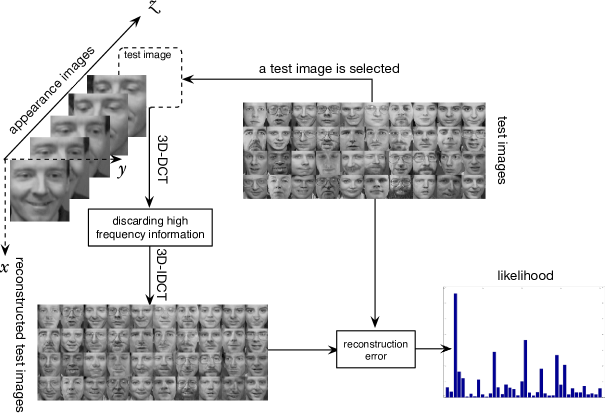
Figure 5: Example of computing the likelihood scores between test images and training images. The left part shows the training image sequence; the top-right part displays the test images; the bottom-middle part exhibits the reconstructed images by 3D-DCT and 3D-IDCT; the bottom-right part plots the corresponding likelihood scores (computed by Equ. (19)).

Specifically, we first compute the $K$-nearest neighbors (referred to as $\mathcal{F}_{+}^{K}\in\mathcal{R}^{N_{1}\times N_{2}\times K}$ and $\mathcal{F}_{-}^{K}\in\mathcal{R}^{N_{1}\times N_{2}\times K}$) of the candidate sample $\tau$ from $\mathcal{F}_{+}$ and $\mathcal{F}_{-}$, sort them by their sum-squared distance to $\tau$ (as shown in the top-left part of Fig. 4), and then utilize the incremental 3D-DCT algorithm to construct the compact object representation. Let $\mathcal{F}_{+}^{{}^{\prime}}$ and $\mathcal{F}_{-}^{{}^{\prime}}$ denote the concatenations of $(\mathcal{F}_{+}^{K},\tau)$ and $(\mathcal{F}_{-}^{K},\tau)$, respectively. Through the incremental 3D-DCT algorithm, the corresponding 3D-DCT coefficient matrices $\mathbf{C}^{{}^{\prime}}_{\mathbf{III}_{+}}$ and $\mathbf{C}^{{}^{\prime}}_{\mathbf{III}_{-}}$ can be efficiently calculated. After discarding the high-frequency coefficients, we can obtain the corresponding compact 3D-DCT coefficient matrices $\mathbf{C}^{\ast}_{\mathbf{III}_{+}}$ and $\mathbf{C}^{\ast}_{\mathbf{III}_{-}}$. Based on Equ. (16), the reconstructed representations of $\mathcal{F}_{+}^{{}^{\prime}}$ and $\mathcal{F}_{-}^{{}^{\prime}}$ are obtained as $\mathcal{F}^{\ast}_{+}$ and $\mathcal{F}^{\ast}_{-}$, respectively. We compute the following reconstruction likelihoods:

$$\begin{array}[]{l}\mathcal{L}_{\tau_{+}}=\exp\left(-\frac{1}{2\gamma^{2}_{+}}\|\tau-f^{\ast}_{\mathbf{III}_{+}}(:,:,K+1)\|^{2}\right),\\ \mathcal{L}_{\tau_{-}}=\exp\left(-\frac{1}{2\gamma^{2}_{-}}\|\tau-f^{\ast}_{\mathbf{III}_{-}}(:,:,K+1)\|^{2}\right),\end{array}$$ (19)

where $\gamma_{+}$ and $\gamma_{-}$ are two scaling factors, $f^{\ast}_{\mathbf{III}_{+}}(:,:,K+1)$ and $f^{\ast}_{\mathbf{III}_{-}}(:,:,K+1)$ are respectively the last images of $\mathcal{F}^{\ast}_{+}$ and $\mathcal{F}^{\ast}_{-}$. Figs. 4 and 5 illustrates the process of computing the reconstruction likelihood between test samples and training samples (i.e., car and face samples) using the 3D-DCT and 3D-IDCT. Based on $\mathcal{L}_{\tau_{+}}$ and $\mathcal{L}_{\tau_{-}}$, we define the final likelihood evaluation criterion:

$$\begin{array}[]{ll}\mathcal{L}^{\ast}_{\tau}&=\rho\left(\mathcal{L}_{\tau_{+}}-\lambda\mathcal{L}_{\tau_{-}}\right)\\ \end{array}$$ (20)

where $\lambda$ is a weight factor and $\rho(x)=\frac{1}{1+\exp(-x)}$ is the sigmoid function.

To demonstrate the discriminative ability of the proposed 3D-DCT based observation model, we plot a confidence map defined in the entire image search space (shown in Fig. 6(a)). Each element of the confidence map is computed by measuring the likelihood score of the candidate bounding box centered at this pixel belonging to the learned observation model, according to Equ. (20). For better visualization, $\mathcal{L}^{\ast}_{\tau}$ is normalized to [0, 1]. After calculating all the normalized likelihood scores at different locations, we have a confidence map which is shown in Fig. 6(b). From Fig. 6(b), we can see that the confidence map has an obvious uni-modal peak, which indicates that the proposed observation model has a good discriminative ability in this image.

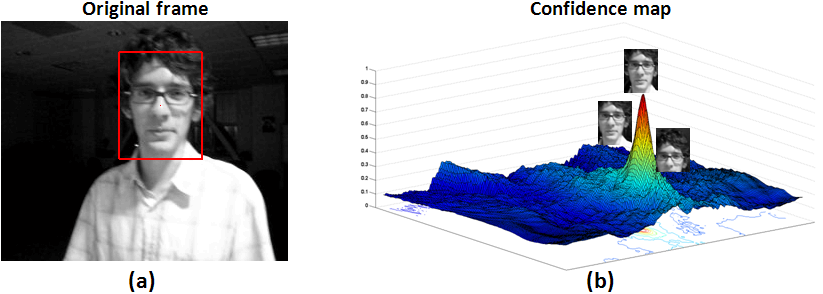
Figure 6: Demonstration of the discriminative ability of the 3D-DCT based object representation used by our tracker. (a) shows the original frame; and (b) displays a confidence map, each element of which corresponds to an image patch in the entire image search space.

IV-C Motion estimation

The motion estimation module is based on a particle filter [43] that is a Markov model with hidden state variables. The particle filter can be divided into the prediction and the update steps:

$$p(\mathbf{Z}_{t}\mid\mathcal{O}_{t-1})\propto\int p(\mathbf{Z}_{t}\mid\mathbf{Z}_{t-1})p(\mathbf{Z}_{t-1}\mid\mathcal{O}_{t-1})d\mathbf{Z}_{t-1},$$

$$p(\mathbf{Z}_{t}\mid\mathcal{O}_{t})\propto p(o_{t}\mid\mathbf{Z}_{t})p(\mathbf{Z}_{t}\mid\mathcal{O}_{t-1}),$$

where $\mathcal{O}_{t}=\{o_{1},\ldots,o_{t}\}$ are observation variables, $p(o_{t}\mid\mathbf{Z}_{t})$ denotes the observation model, and $p(\mathbf{Z}_{t}\mid\mathbf{Z}_{t-1})$ represents the state transition model. For the sake of computational efficiency, we only consider the motion information in translation and scaling. Specifically, let $\mathbf{Z}_{t}=(\mathcal{X}_{t},\mathcal{Y}_{t},\mathcal{S}_{t})$ denote the motion parameters including $\mathcal{X}$ translation, $\mathcal{Y}$ translation, and scaling. The motion model between two consecutive frames is assumed to be a Gaussian distribution:

$$p(\mathbf{Z}_{t}|\mathbf{Z}_{t-1})=\mathcal{N}(\mathbf{Z}_{t};\mathbf{Z}_{t-1},\Sigma),$$ (21)

where $\Sigma$ denotes a diagonal covariance matrix with diagonal elements: $\sigma_{\mathcal{X}}^{2}$, $\sigma_{\mathcal{Y}}^{2}$, and $\sigma_{\mathcal{S}}^{2}$. For each state $\mathbf{Z}_{t}$, there is a corresponding image region $o_{t}$ that is normalized to $N_{1}\times N_{2}$ pixels by image scaling. The likelihood $p(o_{t}\mid\mathbf{Z}_{t})$ is defined as: $p(o_{t}\mid\mathbf{Z}_{t})\propto\mathcal{L}^{\ast}_{\tau}$ where $\mathcal{L}^{\ast}_{\tau}$ is defined in Equ. (20). Thus, the optimal object state $\mathbf{Z}_{t}^{\ast}$ at time $t$ can be determined by solving the following maximum a posterior (MAP) problem:

$$\mathbf{Z}_{t}^{\ast}=\underset{\mathbf{Z}_{t}}{\arg\max}\thinspace p(\mathbf{Z}_{t}\mid\mathcal{O}_{t}).$$ (22)

V Experiments

V-A Data description and implementation details

We evaluate the performance of the proposed tracker (referred to as ITDT) on twenty video sequences, which are captured in different scenes and composed of 8-bit grayscale images. In these video sequences, several complicated factors lead to drastic appearance changes of the tracked objects, including illumination variation, occlusion, out-of-plane rotation, background distraction, small target, motion blurring, pose variation, etc. In order to verify the effectiveness of the proposed tracker on these video sequences, a large number of experiments are conducted. These experiments have two main goals: to verify the robustness of the proposed ITDT in various challenging situations, and to evaluate the adaptive capability of ITDT in tolerating complicated appearance changes.

The proposed ITDT is implemented in Matlab on a workstation with an Intel Core 2 Duo 2.66GHz processor and 3.24G RAM. The average running time of the proposed ITDT is about 0.8 second per frame. During tracking, the pixels values of each frame are normalized into $[0,1]$. For the sake of computational efficiency, we only consider the object state information in 2D translation and scaling in the particle filtering module, where the particle number is set to 200. Each particle is associated with an image patch. After image scaling, the image patch is normalized to $N_{1}\times N_{2}$ pixels. In the experiments, the parameters $(N_{1},N_{2})$ are chosen as $(30,30)$. The scaling factors ($\gamma_{+}$, $\gamma_{-}$) in Equ. (19) are both set to 1.2. The weight factor $\lambda$ in Equ. (20) is set to 0.1. The number of nearest neighbors $K$ in Algorithm 2 is chosen as 15. The parameter $\mathbb{T}$ (i.e., maximum buffer size) in Algorithm 2 is set to 500. These parameter settings remain the same throughout all the experiments in the paper. As for the user-defined tasks on different video sequences, these parameter settings can be slightly readjusted to achieve a better tracking performance.

V-B Competing trackers

We compare the proposed tracker with several other state-of-the-art trackers qualitatively and quantitatively. The competing trackers are referred to as FragT (Fragment-based tracker [10]), MILT (multiple instance boosting-based tracker [34]), VTD (visual tracking decomposition [20]), OAB (online AdaBoost [30]), IPCA (incremental PCA [1]), and L1T ($\ell_{1}$ tracker [15]). Furthermore, IPCA, VTD, and L1T make use of particle filters for state inference while FragT, MILT, and OAB utilize the strategy of sliding window search for state inference. We directly use the public source codes of FragT, MILT, VTD, OAB, IPCA, and L1T. In the experiments, OAB has two different versions, i.e., OAB1 and OAB5, which utilize two different positive sample search radiuses (i.e., $r=1$ and $r=5$ selected in the same way as [34]) for learning AdaBoost classifiers.

We select these seven competing trackers for the following reasons. First, as a recently proposed discriminant learning-based tracker, MILT takes advantage of multiple instance boosting for object/non-object classification. Based on the multi-instance object representation, MILT is capable of capturing the inherent ambiguity of object localization. In contrast, OAB is based on online single-instance boosting for object/non-object classification. The goal of comparing ITDT with MILT and OAB is to demonstrate the discriminative capabilities of ITDT in handling large appearance variations. In addition, based on a fragment-based object representation, FragT is capable of fully capturing the spatial layout information of the object region, resulting in the tracking robustness. Based on incremental principal component analysis, IPCA constructs an eigenspace-based observation model for visual tracking. L1T converts the problem of visual tracking to that of sparse approximation based on $\ell_{1}$-regularized minimization. As a recently proposed tracker, VTD uses sparse principal component analysis to decompose the observation (or motion) model into a set of basic observation (or motion) models, each of which covers a specific type of object appearance (or motion). Thus, comparing ITDT with FragT, IPCA, L1T, and VTD can show their capabilities of tolerating complicated appearance changes.

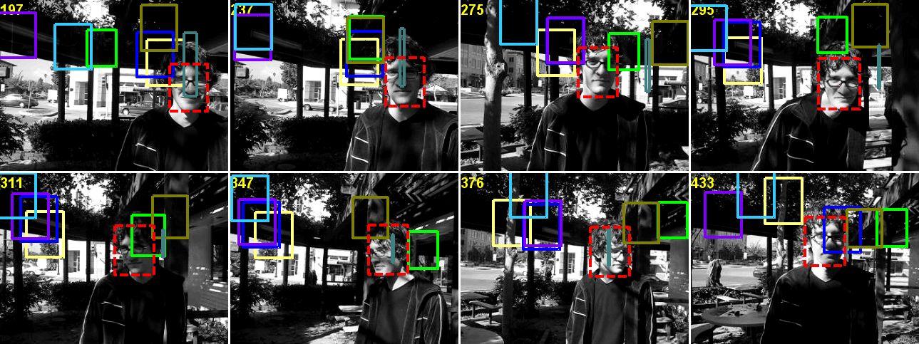
Figure 7: The tracking results of the eight trackers over the representative frames (i.e., the 197th, 237th, 275th, 295th, 311th, 347th, 376th, and 433rd frames) of the “trellis70” video sequence in the scenarios with drastic illumination changes and head pose variations.

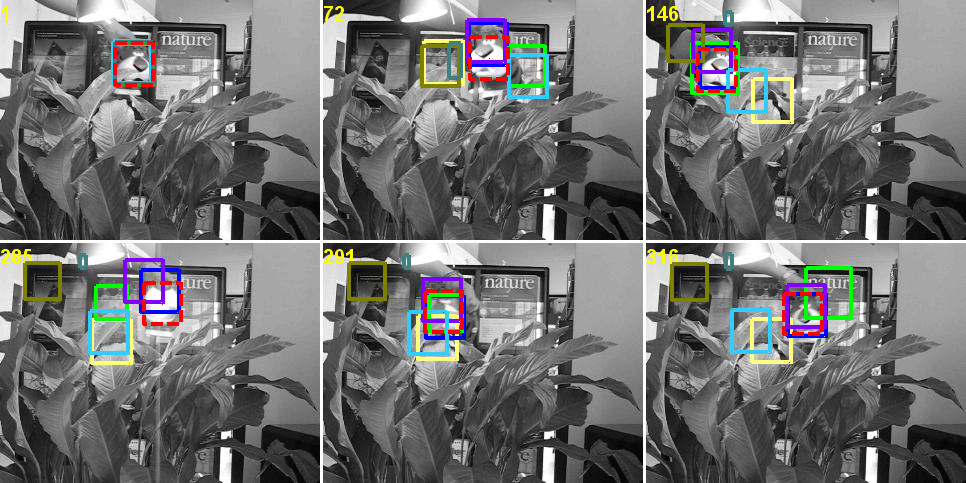
Figure 8: The tracking results of the eight trackers over the representative frames (i.e., the 1st, 72nd, 146th, 285th, 291st, and 316th frames) of the “tiger” video sequence in the scenarios with partial occlusion, illumination change, pose variation, and motion blurring.

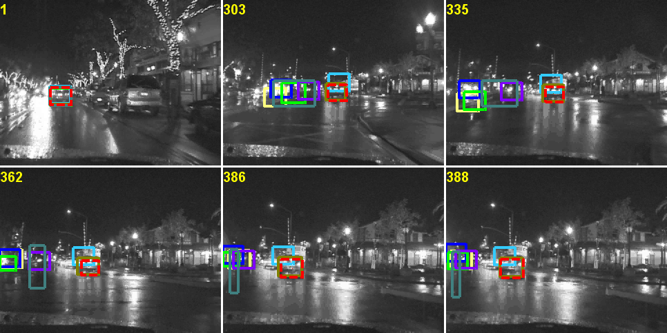
Figure 9: The tracking results of the eight trackers over the representative frames (i.e., the 1st, 303rd, 335th, 362nd, 386th, and 388th frames) of the “car11” video sequence in the scenarios with varying lighting conditions and background clutters.

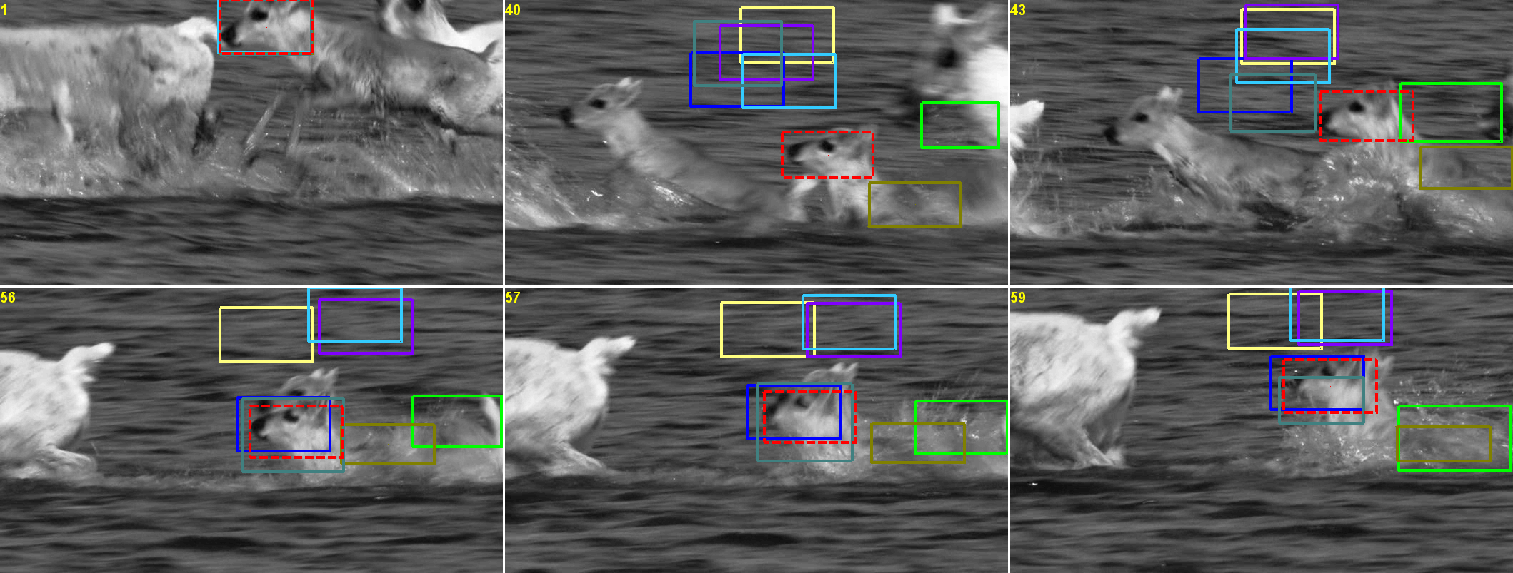
Figure 10: The tracking results of the eight trackers over the representative frames (i.e., the 1st, 40th, 43rd, 56th, 57th, and 59th frames) of the “animal” video sequence in the scenarios with motion blurring and background distraction.

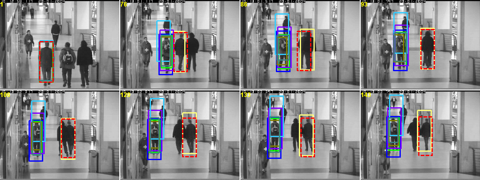
Figure 11: The tracking results of the eight trackers over the representative frames (i.e., the 1st, 76th, 86th, 93rd, 106th, 120th, 133rd, and 143rd frames) of the “sub-three-persons” video sequence in the scenarios with severe occlusions.

Figure 12: The tracking results of the eight trackers over the representative frames (i.e., the 1st, 154th, 204th, 283rd, 330th, and 393rd frames) of the “woman” video sequence in the scenarios with partial occlusions and body pose variations.

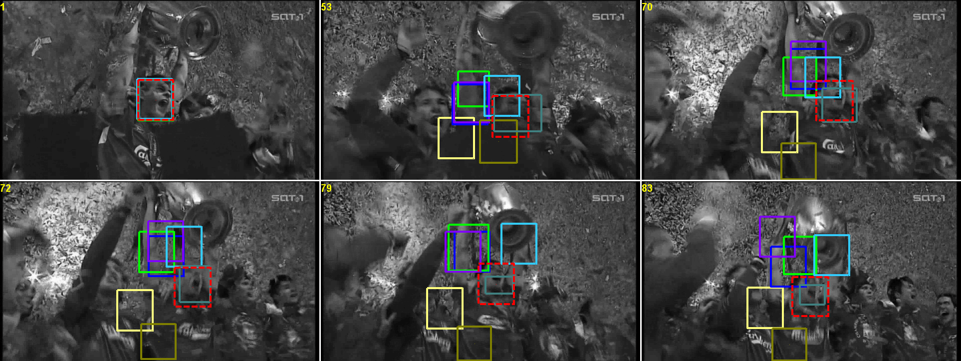
Figure 13: The tracking results of the eight trackers over the representative frames (i.e., the 1st, 53rd, 70th, 72nd, 79th, and 83rd frames) of the “soccer” video sequence in the scenarios with partial occlusions, head pose variations, background clutters, and motion blurring.

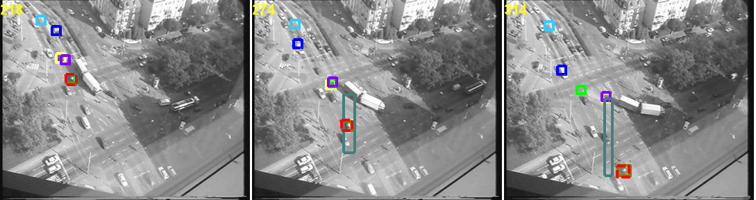
Figure 14: The tracking results of the eight trackers over the representative frames (i.e., the 218th, 274th, and 314th frames) of the “video-car” video sequence in the scenarios with small target and background clutter.

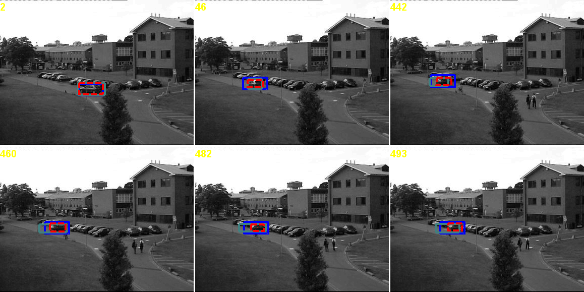
Figure 15: The tracking results of the three best trackers (i.e., ITDT, MILT, and L1T for a better visualization) over the representative frames (i.e., the 2nd, 46th, 442nd, 460th, 482nd, and 493rd frames) of the “pets-car” video sequence in the scenarios with partial occlusion and car pose variation.

V-C Tracking results

Due to space limit, we only report tracking results for the eight trackers (highlighted by the bounding boxes in different colors) over representative frames of the first twelve video sequences, as shown in Figs. 7–18 (the caption of each figure includes the name of its corresponding video sequence). Complete quantitative comparisons for all the twenty video sequences can be found in Tab. I.

As shown in Fig. 7, a man walks under a treillage. Suffering from large changes in environmental illumination and head pose, VTD and OAB5 start to fail in tracking the face after the 170th frame while OAB1, IPCA, MILT, and FragT break down after the 182nd, 201st, 202nd, and 205th frames, respectively. L1T fails to track the face from the 252nd frame. In contrast to these competing trackers, the proposed ITDT is able to successfully track the face till the end of the video.

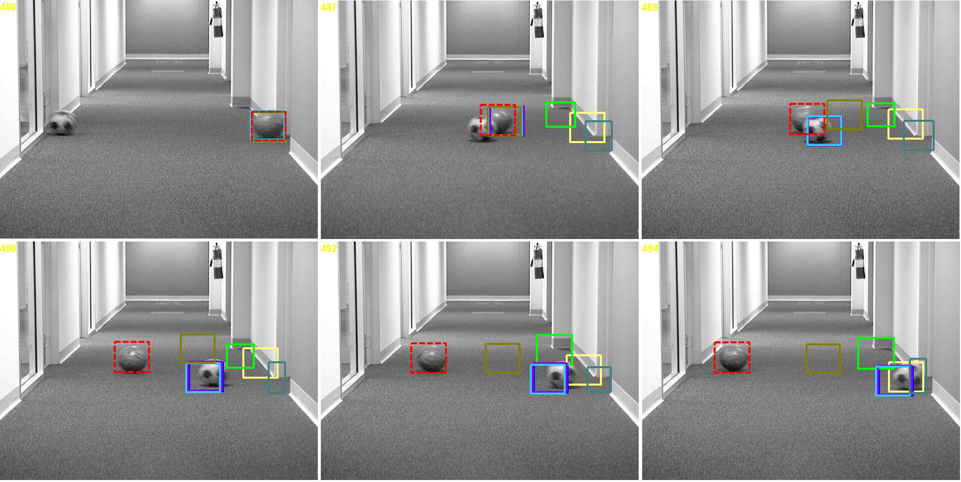
Figure 16: The tracking results of the eight trackers over the representative frames (i.e., the 1st, 8th, 9th, 11th, 13th, and 15th) of the “TwoBalls” video sequence in the scenarios with severe occlusions and motion blurring.

Fig. 8 shows that a tiger toy is shaken strongly. Affected by drastic pose variation, illumination change, and partial occlusion, L1T, IPCA, OAB5, and FragT fail in tracking the tiger toy after the 72nd, 114th, 154th, and 224th frames, respectively. From the 113th frame, VTD fails to track the tiger toy intermittently. OAB1 is not lost in tracking the tiger toy, but it achieves inaccurate tracking results. In contrast, both MILT and ITDT are capable of accurately tracking the tiger toy in the situations of illumination changes and partial occlusions.

As shown in Fig. 9, there is a car moving quickly in a dark road scene with background clutter and varying lighting conditions. After the 271st frame, VTD fails to track the car due to illumination changes. Distracted by background clutter, MILT, FragT, L1T, and OAB1 break down after the 196th, 208th, 286th, and 295th frames, respectively. OAB5 can keep tracking the car, but obtain inaccurate tracking results. In contrast, only ITDT and IPCA succeed in accurately tracking the car throughout the video sequence.

Fig. 10 shows that several deer run and jump in a river. Because of drastic pose variation and motion blurring, FragT fails in tracking the head of a deer after the 5th frame while IPCA, VTD, OAB1, and OAB5 lose the head of the deer after the 13th, 17th, 39th, and 52nd frames, respectively. L1T and MILT are incapable of accurately tracking the head of the deer all the time, and lose the target intermittently. Compared with these trackers, the proposed ITDT is able to accurately track the head of the deer throughout the video sequence.

In the video sequence shown in Fig. 11, several persons walk along a corridor. One person is occluded severely by the other two persons. All the competing trackers except for FragT and ITDT suffer from severe occlusion taking place between the 56th frame and the 76th frame. As a result, they fail to track the person after the 76th frame thoroughly. On the contrary, FragT and ITDT can track the person successfully. However, FragT achieves less accurate tracking results than ITDT.

Figure 17: The tracking results of the three best trackers (i.e., ITDT, L1T, and VTD for a better visualization) over the representative frames (i.e., the 112th, 194th, 237th, 312th, 442nd, 460th, 464th, and 468th frames) of the “girl” video sequence in the scenarios with severe occlusion, in-plane/out-of-plane rotation, and head pose variation.

Fig. 12 shows that woman with varying body poses walks along a pavement. In the meantime, her body is occluded by several cars. After the 127th frame, MILT, OAB1, IPCA, and VTD start to drift away from the woman as a result of partial occlusion. L1T begins to lose the woman after the 147th frame while OAB5 fails to track the woman from the 205th frame. From the 227th frame, FragT stays far away from the woman. Only ITDT can keep tracking the woman over time.

In the video sequence shown in Fig. 13, a number of soccer players assemble together and scream excitedly, jumping up and down. Moreover, their heads are partially occluded by many pieces of floating paper. FragT, IPCA, MILT, and OAB5 fail to track the face from the 49th, 52nd, 49th, and 87th frames, respectively. From the 48th frame to the 94th frame, VTD and OAB1 achieve unsuccessful tracking performances. After the 94th frame, they capture the location of the face again. Compared with these competing trackers, the proposed ITDT can achieve good performance throughout the video sequence.

In Fig. 14, several small-sized cars densely surrounded by other cars move in a blurry traffic scene. Due to the influence of background distraction and small target, MILT, OAB5, FragT, OAB1, VTD, and L1T fail to track the car from the 69th, 160th, 190th, 196th, 246th, and 314th frames, respectively. In contrast, both ITDT and IPCA are able to locate the car accurately at all times.

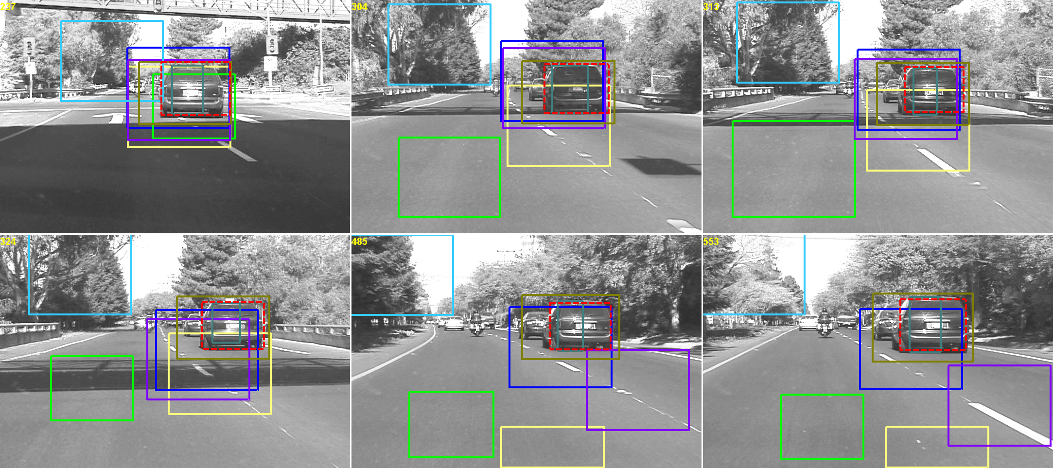
Figure 18: The tracking results of the eight trackers over the representative frames (i.e., the 237th, 304th, 313th, 324th, 485th, and 553rd frames) of the “car4” video sequence in the scenarios with shadow disturbance and pose variation.

As shown in Fig. 15, a driver tries to parallel park in the gap between two cars. At the end of the video sequence, the car is partially occluded by another car. FragT, VTD, OAB1, and IPCA achieve inaccurate tracking performances after the 122nd frame. Subsequently, they begin to drift away after the 435th frame, while OAB5 begins to break down from the 486th frame. MILT and L1T are able to track the car, but achieve inaccurate tracking results. In contrast to these competing trackers, the proposed ITDT is able to perform accurate car tracking throughout the video.

Fig. 16 shows that two balls are rolled on the floor. In the middle of the video sequence, one ball is occluded by the other ball. L1T, FragT and VTD fail in tracking the ball in the 3rd, 5th, and 6th frames, respectively. Before the 8th frame, OAB1, OAB5, MILT, and IPCA achieves inaccurate tracking results. After that, IPCA fails to track the ball thoroughly while OAB1, OAB5, and MILT are distracted by another ball due to severe occlusion. In contrast, only ITDT can successfully track the ball continuously even in the case of severe occlusion.

In the video sequence shown in Fig. 17, a girl rotates her body drastically. At the end, her face is occluded by the other person’s face. Suffering from severe occlusion, IPCA fails to track the face from the 442nd frame while OAB5 begins to break down after the 486th frame. Due to the influence of the head’s out-of-plane rotation, MILT, OAB1, OAB5, FragT, and L1T obtain inaccurate tracking results from the 88th frame to the 265th frame. VTD can track the face persistently, but achieves inaccurate tracking results in most frames. On the contrary, the proposed ITDT can achieve accurate tracking results throughout the video sequence.

As shown in Fig. 18, a car is moving in a highway. Due to the influence of both shadow disturbance and pose variation, OAB5 and OAB1 fail to track the car thoroughly after the 241st and 331st frames, respectively. In contrast, VTD is able to track the car before the 240th frame. However, it tracks the car inaccurately or unsuccessfully after the 240th frame. MILT begin to achieve inaccurate tracking results after the 323rd frame. In contrast, ITDT can track the car accurately in the situations of shadow disturbance and pose variation throughout the video sequence, while both IPCA and L1T achieve less accurate tracking results than ITDT.

V-D Quantitative comparison

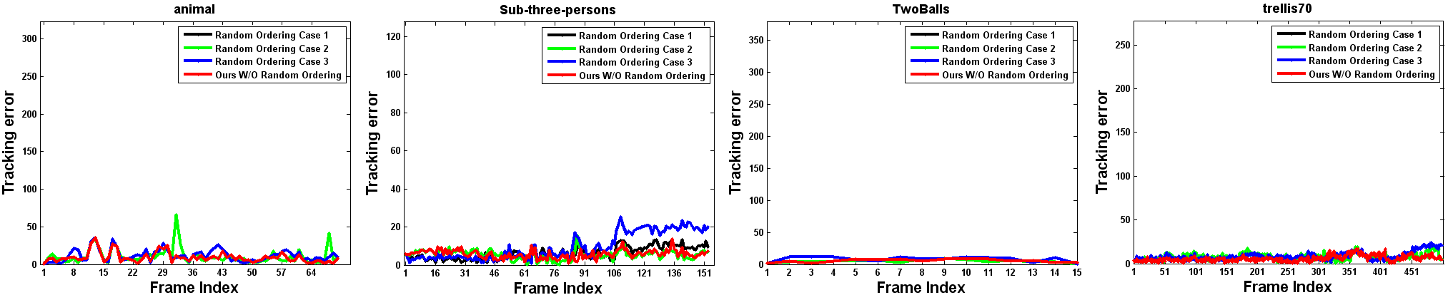
Figure 19: Quantitative tracking performances using different cases of “temporal ordering” (obtained by small-scale random permutation) on the four video sequences. The error curves of the four video sequences in this figure have the same y-axis scale as those of the four video sequences in Fig. 22.

V-D1 Evaluation criteria

For all the twenty video sequences, the object center locations are labeled manually and used as the ground truth. Hence, we can quantitatively evaluate the performances of the eight trackers by computing their pixel-based tracking location errors from the ground truth.

In order to better evaluate the quantitative tracking performance of each tracker, we define a criterion called the tracking success rate (TSR) as: $\mbox{TSR}=\frac{N_{s}}{N}$. Here $N$ is the total number of the frames from a video sequence, and $N_{s}$ is the number of the frames in which a tracker can successfully track the target. The larger the value of TSR is, the better performance the tracker achieves. Furthermore, we introduce an evaluation criterion to determine the success or failure of tracking in each frame: $\frac{\mbox{TLE}}{\mbox{max}\left(W,H\right)}$, where TLE is the pixel-based tracking location error with respect to the ground truth, $W$ is the width of the ground truth bounding box for object localization, and $H$ is the height of the ground truth bounding box. If $\frac{\mbox{TLE}}{\mbox{max}\left(W,H\right)}<0.25$, the tracker is considered to be successful; otherwise, the tracker fails. For each tracker, we compute its corresponding TSRs for all the video sequences. These TSRs are finally used as the criterion for the quantitative evaluation of each tracker.

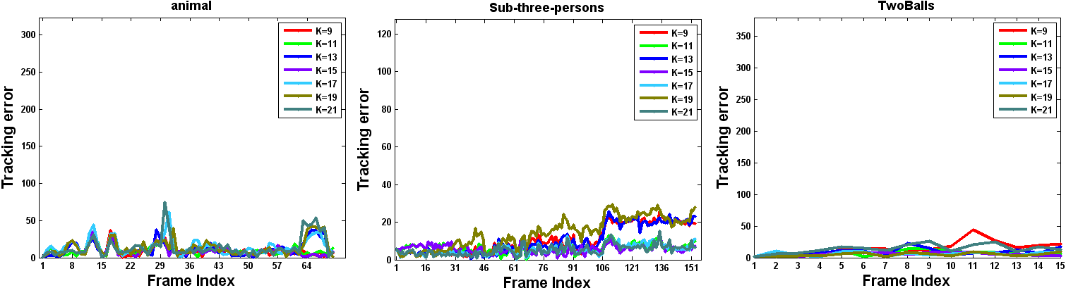
Figure 20: Quantitative tracking performances using different choices of $K$ on the three video sequences. The error curves of the three video sequences in this figure have the same y-axis scale as those of the three video sequences in Fig. 22.

V-D2 Investigation of nearest neighbor construction

The $K$ nearest neighbors used in our 3D-DCT representation are always ordered according to their distances to the current sample (as described in Sec. IV-B). In order to examine the influence of sorting such $K$ nearest neighbors, we randomly exchange a few of them and perform the tracking experiments again, as shown in Fig. 19. It is seen from Fig. 19 that the tracking performances using different ordering cases are close to each other.

In order to evaluate the effect of nearest neighbor selection, we conduct one experiment on three video sequences using difference choices of $K$ such that $K\in\{9,11,13,15,17,19,21\}$, as shown in Fig. 20. From Fig. 20, we can see that the tracking performances using different configurations of $K$ within a certain range are close to each other. Therefore, our 3D-DCT representation is not very sensitive to the choice of $K$ which lies in a certain interval.

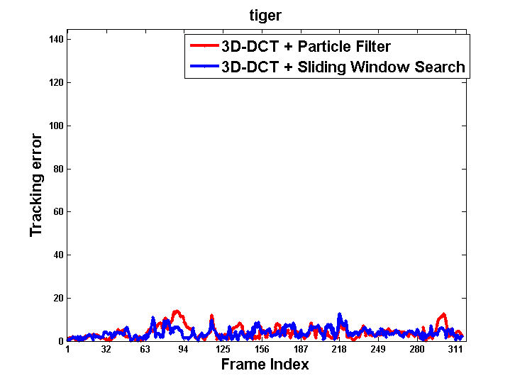
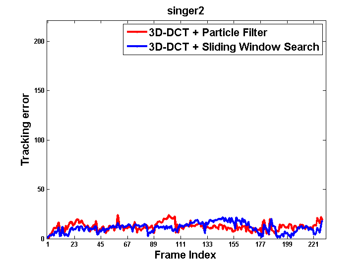
Figure 21: Quantitative tracking performances of different state inference methods, i.e., sliding window search-based object tracking (referred to as “3D-DCT+Sliding Window Search”) and its comparison with particle filter-based tracking (referred to as “3D-DCT + Particle Filter”) on the three video sequences. The error curves of the three video sequences in this figure have the same y-axis scale as those of the three video sequences in Fig. 22 and the supplementary file. Clearly, their tracking performances are almost consistent with each other.

V-D3 Comparison of object representation and state inference

From Tab. I, we see that our tracker achieves equal or higher tracking accuracies than the competing trackers in most cases. Moreover, our tracker utilizes the same state inference method (i.e., particle filter) as IPCA, L1T, and VTD. Consequently, our 3D-DCT object representation play a more critical role in improving the tracking performance than those of IPCA, L1T, and VTD.

Furthermore, we make a performance comparison between our particle filter-based method (referred to as “3D-DCT + Particle Filter”) and a simple state inference method (referred to as “3D-DCT + Sliding Window Search”). Clearly, Fig. 21 shows that the tracking performances of two state inference methods are close to each other. Besides, Tab. I shows that our “3D-DCT + Particle Filter” obtains more accurate tracking results than those of MILT and OAB, which also use a sliding window for state inference. Therefore, we conclude that the 3D-DCT object representation is mostly responsible for the enhanced tracking performance relative to MILT and OAB.

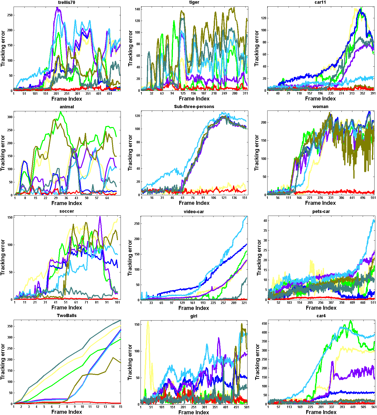
Figure 22: The tracking location error plots obtained by the eight trackers over the first twelve videos. In each sub-figure, the x-axis corresponds to the frame index number, and the y-axis is associated with the tracking location error.

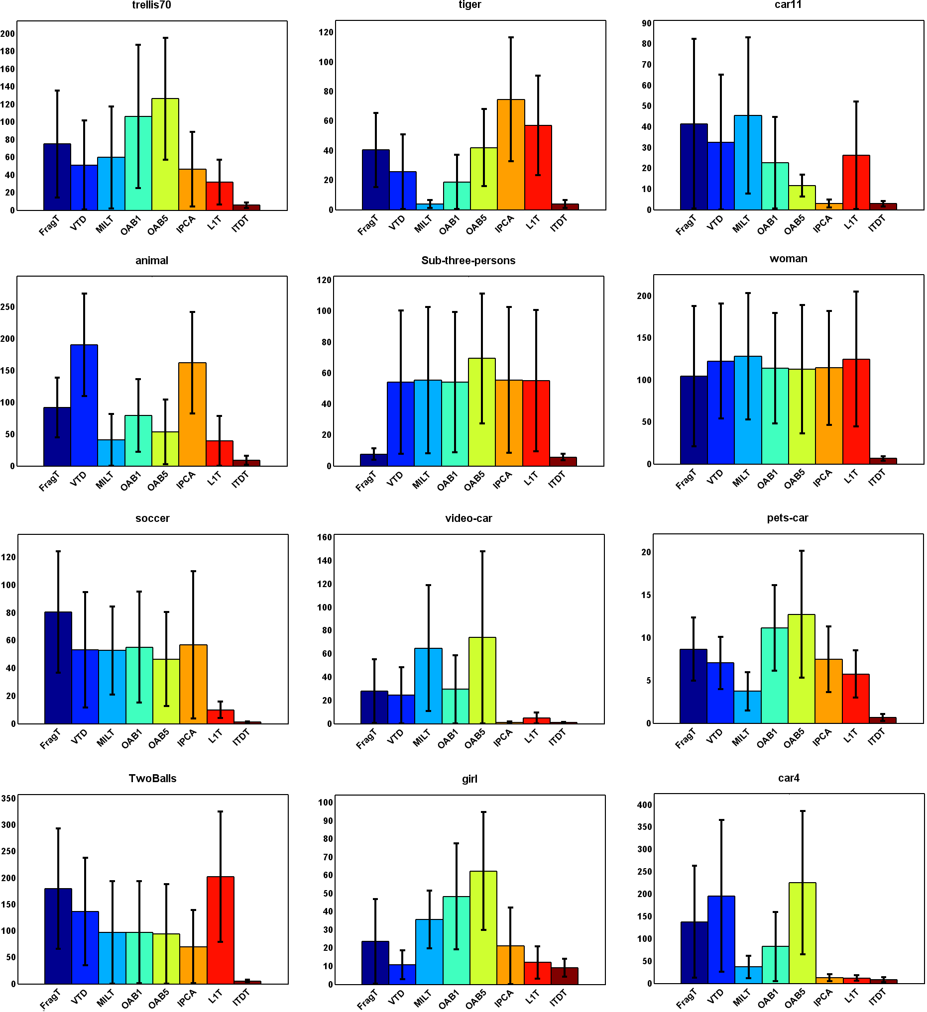
Figure 23: The quantitative comparison results of the eight trackers over the first twelve videos. The figure reports the mean and standard deviation of their tracking location errors over the first twelve videos. In each sub-figure, the x-axis shows the competing trackers, the y-axis is associated with the means of their tracking location errors, and the error bars correspond to the standard deviations of their tracking location errors.

V-D4 Comparison of competing trackers

Fig. 22 plots the tracking location errors (highlighted in different colors) obtained by the eight trackers for the first twelve video sequences. Furthermore, we also compute the mean and standard deviation of the tracking location errors for the first twelve video sequences, and report the results in Fig. 23.

Moreover, Tab. I reports all the corresponding TSRs of the eight trackers over the total twenty video sequences. From Tab. I, we can see that the mean and standard deviation of the TSRs obtained by the proposed ITDT is respectively 0.9802 and 0.0449, which are the best among all the eight trackers. The proposed ITDT also achieves the largest TSR over 19 out of 20 video sequences. As for the “surfer” video sequence, the proposed ITDT is slightly inferior to the best MILT (i.e., 1.33% difference). We believe this is because in the “surfer” video sequence, the tracked object (i.e., the surfer’s head) has an low-resolution appearance with drastic motion blurring. In addition, the surfer’s body has a similar color appearance to the tracked object, which usually leads to the distraction of the trackers using color information. Furthermore, the tracked object’s appearance is varying greatly due to the influence of pose variation and out-of-plane rotation. Under such circumstances, the trackers using local features are usually more effective than those using global features. Therefore, the MILT using Haar-like features slightly outperforms the proposed ITDT using color features in the “surfer” video sequence. In summary, the 3D-DCT based object representation used by the proposed ITDT is able to exploit the correlation between the current appearance sample and the previous appearance samples in the 3D-DCT reconstruction process, and encodes the discriminative information from object/non-object classes. This may have contributed to the tracking robustness in complicated scenarios (e.g., partial occlusions and pose variations).

TABLE I: The quantitative comparison results of the eight trackers over the twenty video sequences. The table reports their tracking success rates (i.e., TSRs) over each video sequence.

	FragT	VTD	MILT	OAB1	OAB5	IPCA	L1T	ITDT
trellis70	0.2974	0.4072	0.3493	0.2295	0.0339	0.3593	0.3972	1.0000
tiger	0.1672	0.5205	0.9495	0.2808	0.1767	0.1104	0.1451	0.9495
car11	0.4020	0.4326	0.1043	0.3181	0.2799	0.9211	0.5700	0.9898
animal	0.1408	0.0845	0.6761	0.3099	0.5352	0.1690	0.5352	0.9859
sub-three-persons	1.0000	0.4610	0.4481	0.4610	0.2662	0.4481	0.4481	1.0000
woman	0.2852	0.2004	0.2058	0.2148	0.1859	0.2148	0.2509	0.9530
soccer	0.1078	0.3824	0.2941	0.3725	0.4118	0.4902	0.9510	1.0000
video-car	0.4711	0.6353	0.1550	0.4225	0.0578	1.0000	0.9058	1.0000
pets-car	0.2959	0.4062	0.8801	0.1799	0.1199	0.4081	0.6983	1.0000
two-balls	0.1250	0.2500	0.3125	0.3125	0.3750	0.5625	0.1250	1.0000
girl	0.6335	0.9044	0.2211	0.1773	0.1633	0.8466	0.8845	0.9741
car4	0.4139	0.3783	0.4849	0.4547	0.2327	0.9982	1.0000	1.0000
shaking	0.1534	0.2767	0.9918	0.9890	0.8438	0.0110	0.0411	0.9973
pktest02	0.1667	1.0000	1.0000	1.0000	0.2333	1.0000	1.0000	1.0000
davidin300	0.4545	0.7900	0.9654	0.3550	0.4762	1.0000	0.8528	1.0000
surfer	0.2128	0.4149	0.9894	0.3112	0.0399	0.4069	0.2766	0.9761
singer2	0.9304	1.0000	1.0000	0.3783	0.2087	1.0000	0.6739	1.0000
seq-jd	0.8020	0.7723	0.5545	0.5446	0.3168	0.6634	0.2277	0.8020
cubicle	0.7255	0.9020	0.2353	0.4706	0.8627	0.7255	0.6863	1.0000
seq-simultaneous	0.6829	0.3171	0.2927	0.6829	0.6585	0.3171	0.5854	0.9756
mean	0.4234	0.5268	0.5555	0.4233	0.3239	0.5826	0.5629	0.9802
s.t.d.	0.2817	0.2768	0.3382	0.2315	0.2438	0.3360	0.3126	0.0449

VI Conclusion

In this paper, we have proposed an effective tracking algorithm based on the 3D-DCT. In this algorithm, a compact object representation has been constructed using the 3D-DCT, which can produce a compact energy spectrum whose high-frequency components are discarded. The problem of constructing the compact object representation has been converted to that of how to efficiently compress and reconstruct the video data. To efficiently update the object representation during tracking, we have also proposed an incremental 3D-DCT algorithm which decomposes the 3D-DCT into the successive operations of the 2D-DCT and 1D-DCT on the video data. The incremental 3D-DCT algorithm only needs to compute 2D-DCT for newly added frames as well as the 1D-DCT along the time dimension, leading to high computational efficiency. Moreover, by computing and storing the cosine basis functions beforehand, we can significantly reduce the computational complexity of the 3D-DCT. Based on the incremental 3D-DCT algorithm, a discriminative criterion has been designed to measure the information loss resulting from 3D-DCT based signal reconstruction, which contributes to evaluating the confidence score of a test sample belonging to the foreground object. Since considering both the foreground and the background reconstruction information, the discriminative criterion is robust to complicated appearance changes (e.g., out-of-plane rotation and partial occlusion). Using this discriminative criterion, we have conducted visual tracking in the particle filtering framework which propagates sample distributions over time. Compared with several state-of-the-art trackers on challenging video sequences, the proposed tracker is more robust to the challenges including illumination changes, pose variations, partial occlusions, background distractions, motion blurring, complicated appearance changes, etc. Experimental results have demonstrated the effectiveness and robustness of the proposed tracker.

References

- [1] D. A. Ross, J. Lim, R. Lin, and M. Yang, “Incremental learning for robust visual tracking,” Int. J. Computer Vision, vol. 77, no. 1, pp. 125–141, 2008.
- [2] X. Li, W. Hu, Z. Zhang, X. Zhang, M. Zhu, and J. Cheng, “Visual tracking via incremental log-euclidean riemannian subspace learning,” in Proc. IEEE Conf. Computer Vision & Pattern Recognition, 2008, pp. 1–8.
- [3] A. K. Jain, Fundamentals of Digital Image Processing, New Jersey: Prentice Hall Inc., 1989.
- [4] S. A. Khayam, “The discrete cosine transform (DCT): theory and application,” Technical report, Michigan State University, 2003.
- [5] Z. M. Hafed and M. D. Levine, “Face recognition using the discrete cosine transform,” Int. J. Computer Vision, vol. 43, no. 3, pp. 167–188, 2001.
- [6] G. Feng and J. Jiang, “JPEG compressed image retrieval via statistical features,” Pattern Recognition, vol. 36, no. 4, pp. 977–985, 2003.
- [7] D. He, Z. Gu, and N. Cercone, “Efficient image retrieval in dct domain using hypothesis testing,” in Proc. Int. Conf. Image Processing, 2009, pp. 225–228.
- [8] D. Chen, Q. Liu, M. Sun, and J. Yang, “Mining appearance models directly from compressed video,” IEEE Trans. Multimedia, vol. 10, no. 2, pp. 268–276, 2008.
- [9] Y. Zhong, H. Zhang, and A. K. Jain, “Automatic caption localization in compressed video,” IEEE Trans. Pattern Analysis & Machine Intelligence, vol. 22, no. 4, pp. 385–392, 2000.
- [10] A. Adam, E. Rivlin, and I. Shimshoni, “Robust fragments-based tracking using the integral histogram,” in Proc. IEEE Conf. Computer Vision & Pattern Recognition, 2006, pp. 798–805.
- [11] C. Shen, J. Kim, and H. Wang, “Generalized kernel-based visual tracking,” IEEE Trans. Circuits & Systems for Video Technology, vol. 20, no. 1, pp. 119–130, 2010.
- [12] H. Wang, D. Suter, K. Schindler, and C. Shen, “Adaptive object tracking based on an effective appearance filter,” IEEE Trans. Pattern Analysis & Machine Intelligence, vol. 29, no. 9, pp. 1661–1667, 2007.
- [13] A. D. Jepson, D. J. Fleet, and T. F. El-Maraghi, “Robust online appearance models for visual tracking,” in Proc. IEEE Conf. Computer Vision & Pattern Recognition, 2001, pp. 415–422.
- [14] X. Li, W. Hu, Z. Zhang, X. Zhang, and G. Luo, “Robust visual tracking based on incremental tensor subspace learning,” in Proc. Int. Conf. Computer Vision, 2007, pp. 1–8.
- [15] X. Mei and H. Ling, “Robust visual tracking and vehicle classification via sparse representation,” IEEE Trans. Pattern Analysis & Machine Intelligence, 2011.
- [16] B. Liu, L. Yang, J. Huang, P. Meer, L. Gong, and C. Kulikowski, “Robust and fast collaborative tracking with two stage sparse optimization,” in Proc. Euro. Conf. Computer Vision, 2010.
- [17] B. Liu, J. Huang, C. Kulikowski, and L. Yang, “Robust tracking using local sparse appearance model and k-selection,” in Proc. IEEE Conf. Computer Vision & Pattern Recognition, 2011.
- [18] H. Li, C. Shen, and Q. Shi, “Real-time visual tracking with compressed sensing,” in Proc. IEEE Conf. Computer Vision & Pattern Recognition, 2011.
- [19] X. Li, C. Shen, Q. Shi, D. Anthony, and A. van den Hengel, “Non-sparse linear representations for visual tracking with online reservoir metric learning,” Proc. IEEE Conf. Computer Vision & Pattern Recognition, 2012.
- [20] J. Kwon and K. M. Lee, “Visual tracking decomposition,” in Proc. IEEE Conf. Computer Vision & Pattern Recognition, 2010, pp. 1269–1276.
- [21] F. Porikli, O. Tuzel, and P. Meer, “Covariance tracking using model update based on lie algebra,” in Proc. IEEE Conf. Computer Vision & Pattern Recognition, 2006, pp. 728–735.
- [22] Y. Wu, J. Cheng, J. Wang, and H. Lu, “Real-time visual tracking via incremental covariance tensor learning,” in Proc. Int. Conf. Computer Vision, 2009, pp. 1631–1638.
- [23] D. Comaniciu, V. Ramesh, and P. Meer, “Kernel-based object tracking,” IEEE Trans. Pattern Analysis & Machine Intelligence, vol. 25, no. 5, pp. 564–577, 2003.
- [24] C. Shen, M. J. Brooks, and A. van den Hengel, “Fast Global Kernel Density Mode Seeking: Applications To Localization And Tracking,” IEEE Trans. Image Processing, vol. 16, no. 5, pp. 1457–1469, 2007.
- [25] W. Qu and D. Schonfeld, “Robust control-based object tracking,” IEEE Trans. Image Processing, vol. 17, no. 9, pp. 1721–1726, 2008.
- [26] S. Avidan, “Support vector tracking,” IEEE Trans. Pattern Analysis & Machine Intelligence, vol. 26, no. 8, pp. 1064–1072, 2004.
- [27] M. Tian, W. Zhang, and F. Liu, “On-line ensemble SVM for robust object tracking,” in Proc. Asian Conf. Computer Vision, 2007, pp. 355–364.
- [28] F. Tang, S. Brennan, Q. Zhao, and H. Tao, “Co-tracking using semi-supervised support vector machines,” in Proc. Int. Conf. Computer Vision, 2007.
- [29] X. Li, A. Dick, H. Wang, C. Shen, and A. van den Hengel, “Graph mode-based contextual kernels for robust svm tracking,” in Proc. Int. Conf. Computer Vision, 2011, pp. 1156–1163.
- [30] H. Grabner, M. Grabner, and H. Bischof, “Real-time tracking via on-line boosting,” in Proc. British Machine Vision Conf., 2006, pp. 47–56.
- [31] H. Grabner, C. Leistner, and H. Bischof, “Semi-supervised on-line boosting for robust tracking,” in Proc. Euro. Conf. Computer Vision, 2008, pp. 234–247.
- [32] R. T. Collins, Y. Liu, and M. Leordeanu, “Online selection of discriminative tracking features,” IEEE Trans. Pattern Analysis & Machine Intelligence, vol. 27, no. 10, pp. 1631–1643, 2005.
- [33] J. Santner, C. Leistner, A. Saffari, T. Pock, and H. Bischof, “Prost: Parallel robust online simple tracking,” in Proc. IEEE Conf. Computer Vision & Pattern Recognition, 2010, pp. 723–730.
- [34] B. Babenko, M. Yang, and S. Belongie, “Visual tracking with online multiple instance learning,” in Proc. IEEE Conf. Computer Vision & Pattern Recognition, 2009, pp. 983–990.
- [35] J. Fan, Y. Wu, and S. Dai, “Discriminative spatial attention for robust tracking,” in Proc. Euro. Conf. Computer Vision, 2010, pp. 480–493.
- [36] X. Wang, G. Hua, and T. X. Han, “Discriminative tracking by metric learning,” in Proc. Euro. Conf. Computer Vision, 2010, pp. 200–214.
- [37] N. Jiang, W. Liu, and Y. Wu, “Learning adaptive metric for robust visual tracking,” IEEE Trans. Image Processing, vol. 20, no. 8, pp. 2288–2300, 2011.
- [38] M. Yang, Z. Fan, J. Fan, and Y. Wu, “Tracking non-stationary visual appearances by data-driven adaptation,” IEEE Trans. Image Processing, vol. 18, no. 7, pp. 1633–1644, 2009.
- [39] X. Liu and T. Yu, “Gradient feature selection for online boosting,” in Proc. Int. Conf. Computer Vision, 2007, pp. 1–8.
- [40] S. Avidan, “Ensemble tracking,” IEEE Trans. Pattern Analysis & Machine Intelligence, vol. 29, no. 2, pp. 261–271, 2007.
- [41] L. D. Lathauwer, B. Moor, and J. Vandewalle, “On the best rank-1 and rank- approximation of higher-order tensors,” SIAM Journal of Matrix Analysis and Applications, vol. 21, no. 4, pp. 1324–1342, 2000.
- [42] J. Wang, J. Yang, K. Yu, F. Lv, T. Huang, and Y. Gong, “Locality-constrained linear coding for image classification,” in Proc. IEEE Conf. Computer Vision & Pattern Recognition, 2010, pp. 3360–3367.
- [43] M. Isard and A. Blake, “Contour tracking by stochastic propagation of conditional density,” in Proc. Euro. Conf. Computer Vision, 1996, pp. 343–356.