Coefficient of performance under optimized figure of merit in minimally nonlinear irreversible refrigerator

Abstract

We apply the model of minimally nonlinear irreversible heat engines developed by Izumida and Okuda [EPL 97, 10004 (2012)] to refrigerators. The model assumes extended Onsager relations including a new nonlinear term accounting for dissipation effects. The bounds for the optimized regime under an appropriate figure of merit and the tight-coupling condition are analyzed and successfully compared with those obtained previously for low-dissipation Carnot refrigerators in the finite-time thermodynamics framework. Besides, we study the bounds for the nontight-coupling case numerically. We also introduce a leaky low-dissipation Carnot refrigerator and show that it serves as an example of the minimally nonlinear irreversible refrigerator, by calculating its Onsager coefficients explicitly.

1 Introduction

Nowadays, the optimization of thermal heat devices is receiving a special attention because of its straightforward relation with the depletion of energy resources and the concerns of sustainable development. A number of different performance regimes based on different figures of merit have been considered with special emphasis in the analysis of possible universal and unified features. Among them, the efficiency at maximum power (EMP) $\eta_{\rm maxP}$ for heat engines working along cycles or in steady-state is largely the issue most studied independently of the thermal device nature (macroscopic, stochastic or quantum) and/or the model characteristics [1, 2, 3, 4, 5, 6, 7, 8, 9, 10, 11, 12, 13, 14]. Even theoretical results have been faced with an experimental realization for micrometre-sized stochastic heat engines performing a Stirling cycle [15].

For most of the Carnot-like heat engine models analyzed in the finite-time thermodynamics (FTT) framework [5, 6] the EMP regime allows for valuable and simple expressions of the optimized efficiency, which under endoreversible assumptions (i.e., all considered irreversibilities coming from the couplings between the working system and the external heat reservoirs through linear heat transfer laws) recover the paradigmatic Curzon-Ahlborn value [16] $\eta_{\rm maxP}=1-\sqrt{\tau}\equiv\eta_{\rm CA}$ using $\tau\equiv T_{\rm c}/T_{\rm h}$, where $T_{\rm c}$ and $T_{\rm h}$ denote the temperature of the cold and hot heat reservoirs, respectively. A significant conceptual advance was reported by Esposito et al. [17] by considering a low-dissipation Carnot heat engine model. In this model the entropy production in the hot (cold) heat exchange process is assumed to be inversely proportional to the time duration of the process (see eqs. (30) and (31) for more details). Then the reversible regime is approached in the limit of infinite times and the maximum power regime allows us to recover the Curzon-Ahlborn value when symmetric dissipation is considered. This derivation does not require the assumption of any specific heat transfer law nor the small temperature difference. Considering extremely asymmetric dissipation limits, these authors also derived that EMP is bounded from the lower and upper sides as

$$\frac{\eta_{\rm C}}{2}\leq\eta_{{\rm maxP}}\leq\frac{\eta_{\rm C}}{2-\eta_{\rm C}},$$ (1)

where $\eta_{\rm C}\equiv 1-\tau$ is the Carnot efficiency. The Curzon-Ahlborn value $\eta_{\rm CA}$ (i.e., the symmetric dissipation limit) is located between these bounds. Additional studies on various heat engine models [18, 19, 20] confirmed and generalized above results.

Work by de Tomás et al. [21] extended the low dissipation Carnot heat engine model to refrigerators and besides proposed a unified figure of merit ($\chi$-criterion described below) focusing the attention in the common characteristics of every heat energy converter (the working systems and total cycle time) instead of any specific coupling to external heat sources which can vary according to a particular arrangement. For refrigerators, we denote the heat absorbed by the working system from the cold heat reservoir by $Q_{\rm c}$, the heat evacuated from the working system to the hot heat reservoir by $Q_{\rm h}$ and the work input to the working system by $W\equiv Q_{\rm h}-Q_{\rm c}$. For heat engines, we may inversely choose natural directions of heat transfers and work. That is, we denote the heat absorbed by the working system from the hot heat reservoir by $Q_{\rm h}$, the heat evacuated from the working system to the cold heat reservoir by $Q_{\rm c}$ and the work output by $W\equiv Q_{\rm h}-Q_{\rm c}$. Then we can define this $\chi$-criterion as the product of the converter efficiency $z$ times the heat $Q_{\rm in}$ exchanged between the working system and the heat reservoir, divided by the time duration of cycle $t_{\rm cycle}$:

$$\chi=\frac{z\,Q_{\rm in}}{t_{\rm cycle}},$$ (2)

where $Q_{\rm in}=Q_{\rm c}$, $z=\varepsilon\equiv Q_{\rm c}/W$ for refrigerators and $Q_{\rm in}=Q_{\rm h}$, $z=\eta\equiv W/Q_{\rm h}$ for heat engines. It becomes power as $\chi=W/t_{\rm cycle}$ when applied to heat engines and also allows us to obtain the optimized coefficient of performance (COP) $\varepsilon_{{\rm max\chi}}$ under symmetric dissipation conditions when applied to refrigerators [21]:

$$\varepsilon_{{\rm max\chi}}=\sqrt{1+\varepsilon_{\rm C}}-1\equiv\varepsilon_{\rm CA},$$ (3)

where $\varepsilon_{\rm C}\equiv\tau/(1-\tau)$ is the Carnot COP. This result could be considered as the genuine counterpart of the Curzon-Ahlborn efficiency for refrigerators. It was first obtained in FTT for Carnot-like refrigerators by Yan and Chen [22] taking as target function $\varepsilon\dot{Q}_{\rm c}$, where $\dot{Q}_{\rm c}$ is the cooling power of the refrigerator, later and independently by Velasco et al. [23, 24] using a maximum per-unit-time COP and by Allahverdyan et al. [25] in the classical limit of a quantum model with two n-level systems interacting via a pulsed external field. Very recent results by Wang et al. [26] generalized the previous results for refrigerators [21] and they obtained the following bounds of the COP considering extremely asymmetric dissipation limits:

$$0\leq\varepsilon_{{\rm max\chi}}\leq\frac{\sqrt{9+8\varepsilon_{\rm C}}-3}{2}.$$ (4)

These bounds for refrigerators play the same role that eq. (1) for heat engines.

A shortcoming of the all above results is the model dependence. Thus additional research work [27, 28, 29, 30] has been devoted to obtain model-independent results on efficiency and COP using the well founded formalism of linear irreversible thermodynamics (LIT) for both cyclic and steady-state models including explicit calculations of the Onsager coefficients using molecular kinetic theory [31, 32, 33]. Beyond the linear regime a further improvement was reported by Izumida and Okuda [34] by proposing a model of minimally nonlinear irreversible heat engines described by extended Onsager relations with nonlinear terms accounting for power dissipation. The validity of the theory was checked by comparing the results for EMP and its bounds with eq. (1). Now, the main goal of the present paper is to extend the application of this nonlinear irreversible theory [34] to refrigerators and analyze their COP under maximum $\chi$-condition. To get this we first present the model and analyze the results when the tight-coupling condition is met. Then we also study the nontight-coupling case numerically. Finally we extend the low-dissipation Carnot refrigerator model [26] to a leaky model and show that it serves as an example of the minimally nonlinear irreversible refrigerator by calculating its Onsager coefficients explicitly.

2 Minimally nonlinear irreversible refrigerator model

Refrigerators are generally classified into two types, that is, steady-state refrigerators and cyclic ones. Our theory can be applied to both cases. Since the working system stays unchanged for steady-state refrigerators and comes back to the original state after one-cycle for cyclic refrigerators, the entropy production rate $\dot{\sigma}$ of the refrigerators agrees with the entropy increase rate of the heat reservoirs as

$$\dot{\sigma}=\frac{\dot{Q}_{\rm c}+\dot{W}}{T_{\rm h}}-\frac{\dot{Q}_{\rm c}}{T_{\rm c}}=\frac{\dot{W}}{T_{\rm h}}+\dot{Q}_{\rm c}\left(\frac{1}{T_{\rm h}}-\frac{1}{T_{\rm c}}\right),$$ (5)

where the dot denotes the quantity per unit time for steady-state refrigerators and the quantity divided by the time duration of cycle $t_{\rm cycle}$ for cyclic refrigerators. From the decomposition of $\dot{\sigma}$ into the sum of the product of thermodynamic flux $J_{i}$ and its conjugate thermodynamic force $X_{i}$ as $\dot{\sigma}=J_{1}X_{1}+J_{2}X_{2}$, we can define $J_{1}\equiv\dot{x}$, $X_{1}\equiv F/T_{\rm h}$ and $J_{2}\equiv\dot{Q}_{\rm c}$, $X_{2}\equiv 1/T_{\rm h}-1/T_{\rm c}$ for steady-state refrigerators, where $\dot{W}=F\dot{x}$ with $F$ and $x$ denoting the time-independent external generalized force and its conjugate variable, respectively. Likewise we can also define

$$J_{1}\equiv\frac{1}{t_{\rm cycle}},\ X_{1}\equiv\frac{W}{T_{\rm h}},$$ (6)

$$J_{2}\equiv\dot{Q}_{\rm c}=\frac{Q_{\rm c}}{t_{\rm cycle}},\ X_{2}\equiv\frac{1}{T_{\rm h}}-\frac{1}{T_{\rm c}},$$ (7)

for cyclic refrigerators, where $X_{1}$ and $X_{2}$ play the role of driver and driven forces, respectively. 

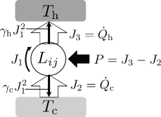
Figure 1: Schematic illustration of the minimally nonlinear irreversible refrigerator described by eqs. (12) and (13).

Anyway, we assume that the refrigerators are described by the following extended Onsager relations [34]:

$$J_{1}=L_{11}X_{1}+L_{12}X_{2},$$ (8)

$$J_{2}=L_{21}X_{1}+L_{22}X_{2}-\gamma_{\rm c}{J_{1}}^{2},$$ (9)

where $L_{ij}$’s are the Onsager coefficients with reciprocity $L_{12}=L_{21}$. The nonlinear term $-\gamma_{\rm c}J_{1}^{2}$ means the power dissipation into the cold heat reservoir and $\gamma_{\rm c}>0$ denotes its strength. We also disregard other possible nonlinear terms by assuming that their coefficients are too small when compared with the power dissipation term.

In the limit of $X_{i}$’s $\to 0$, the thermodynamic forces can be approximated as $X_{1}\simeq W/T$ ($X_{1}=F/T$) and $X_{2}\simeq\Delta T/T^{2}$ for the cyclic (steady-state) refrigerators, where $\Delta T\equiv T_{\rm h}-T_{\rm c}$ and $T\equiv(T_{\rm h}+T_{\rm c})/2$. These expressions of the forces are consistent with [27, 31]. Then the extended Onsager relations in eqs. (8) and (9) recover the usual linear Onsager relations such as in [27, 31]. Thus our minimally nonlinear irreversible model naturally includes the linear irreversible model as a special case. The non-negativity of the entropy production rate $\dot{\sigma}=J_{1}X_{1}+J_{2}X_{2}$, which is a quadratic form of $X_{i}$’s in the linear irreversible model, leads to the restriction of the Onsager coefficients [31, 35, 36] to

$$L_{11}\geq 0,L_{22}\geq 0,L_{11}L_{22}-L_{12}L_{21}\geq 0.$$ (10)

Although our model includes the power dissipation as the nonlinear term, we also assume eq. (10) holds. This idea that the dissipation is included in the scope of the linear irreversible thermodynamics is also found in [37, 38, 39].

The power input $P$ is given by $P\equiv\dot{W}=J_{1}X_{1}T_{\rm h}>0$. Then the heat flux into the hot heat reservoir $\dot{Q}_{\rm h}\equiv P+\dot{Q}_{\rm c}\equiv J_{3}$ is given as

$$J_{3}=P+\dot{Q}_{\rm c}=J_{1}X_{1}T_{\rm h}+J_{2}.$$ (11)

By solving eq. (8) with respect to $X_{1}$ and substituting it into eqs. (9) and (11), we can rewrite $J_{2}$ and $J_{3}$ by using $J_{1}$ instead of $X_{1}$ as (see fig. 1):

$$J_{2}=\frac{L_{21}}{L_{11}}J_{1}+L_{22}(1-q^{2})X_{2}-\gamma_{\rm c}{J_{1}}^{2},$$ (12)

$$J_{3}=\frac{L_{21}}{L_{11}}\frac{T_{\rm h}}{T_{\rm c}}J_{1}+L_{22}(1-q^{2})X_{2}+\gamma_{\rm h}{J_{1}}^{2},$$ (13)

where $q\equiv\frac{L_{12}}{\sqrt{L_{11}L_{22}}}$ is the usual coupling strength parameter ($|q|\leq 1$ from eq. (10)) and $\gamma_{\rm h}$ denotes the strength of the power dissipation into the hot heat reservoir as

$$\gamma_{\rm h}\equiv\frac{T_{\rm h}}{L_{11}}-\gamma_{\rm c}>0.$$ (14)

Eqs. (12) and (13) allow a clearer description of the refrigerator than eqs. (8) and (9) by considering $J_{1}$ as the control parameter instead of $X_{1}$ at constant $X_{2}$. So, each term in eqs. (12) and (13) has explicit physical meanings (see also [34]): the two first terms mean the reversible heat transport between the working system and the heat reservoirs; the second ones account for coupling effects between the heat reservoirs; and the third ones account for the power dissipation ($\sim J_{1}^{2}$) into the heat reservoirs, which inevitably occurs in a finite-time motion ($J_{1}\neq 0$).

Using eqs. (12) and (13) instead of eqs. (8) and (9), the power input $P=J_{3}-J_{2}$ and the entropy production rate $\dot{\sigma}=\frac{J_{3}}{T_{\rm h}}-\frac{J_{2}}{T_{\rm c}}$ are written as

$$P=\frac{L_{21}}{L_{11}}\left(\frac{1}{\tau}-1\right)J_{1}+\frac{T_{\rm h}}{L_{11}}{J_{1}}^{2},$$ (15)

and

$$\dot{\sigma}=L_{22}(1-q^{2})X_{2}^{2}+J_{1}^{2}\left(\frac{\gamma_{\rm c}}{T_{\rm c}}+\frac{\gamma_{\rm h}}{T_{\rm{h}}}\right).$$ (16)

For the refrigerator, the converter efficiency $z$ in eq. (2) is the COP $\varepsilon$ defined as

$$\varepsilon\equiv\frac{\dot{Q}_{\rm c}}{P}=\frac{J_{2}}{P}=\frac{\frac{L_{21}}{L_{11}}J_{1}+L_{22}(1-q^{2})X_{2}-\gamma_{\rm c}J_{1}^{2}}{\frac{L_{21}}{L_{11}}(\frac{1}{\tau}-1)J_{1}+\frac{T_{\rm h}}{L_{11}}J_{1}^{2}},$$ (17)

where we used eqs. (12) and (15). We also introduce the $\chi$-criterion as a product of the COP $\varepsilon$ and the cooling power $J_{2}$, identifying the cooling power $Q_{\rm in}/t_{\rm cycle}$ in eq. (2) as $\dot{Q}_{\rm c}=J_{2}$:

$$\chi=\frac{{J_{2}}^{2}}{P}=\frac{\left(\frac{L_{21}}{L_{11}}J_{1}+L_{22}(1-q^{2})X_{2}-\gamma_{\rm c}{J_{1}}^{2}\right)^{2}}{\frac{L_{21}}{L_{11}}\left(\frac{1}{\tau}-1\right)J_{1}+\frac{T_{\rm h}}{L_{11}}{J_{1}}^{2}},$$ (18)

where we used eqs. (12) and (15). Though eq. (2) using $Q_{\rm in}/t_{\rm cycle}$ appears to be valid only for cyclic heat energy converters, eq. (18) using $J_{2}$ is valid even for steady-state refrigerators. In order to get a positive cooling power $J_{2}>0$, we see from eq. (12) that $J_{1}$ should be located in a finite range as

$$\frac{L_{21}-\sqrt{D}}{2L_{11}\gamma_{\rm c}}<J_{1}<\frac{L_{21}+\sqrt{D}}{2L_{11}\gamma_{\rm c}},$$ (19)

where the discriminant $D$ is given by

$$D\equiv L_{21}^{2}+4L_{11}^{2}L_{22}\gamma_{\rm c}(1-q^{2})X_{2}>0.$$ (20)

We consider the optimization of the $\chi$-criterion with respect to $J_{1}$ in this range. In the following, we first analyze the case $|q|=1$ called the tight-coupling condition. Afterward we consider the nontight-coupling case $|q|\neq 1$.

2.1 Tight-coupling case $|q|=1$

In the tight-coupling case, eq. (19) becomes

$$0<J_{1}<\frac{L_{21}}{\gamma_{\rm c}L_{11}}.$$ (21)

We find $J_{1}=J_{1}^{\rm max\chi}$ which gives the maximum of $\chi$ by solving the equation $\partial\chi/\partial J_{1}=0$. Noticing that $J_{1}=L_{21}/(\gamma_{c}L_{11})$ as the solution of $J_{2}=0$ is always one of the solutions of $\partial\chi/\partial J_{1}=0$, we can simplify that equation to the following quadratic one:

$$J_{1}^{2}+\frac{3L_{21}}{2\varepsilon_{\rm C}T_{\rm h}}J_{1}-\frac{L_{21}^{2}}{2\gamma_{\rm c}L_{11}\varepsilon_{\rm C}T_{\rm h}}=0.$$ (22)

Solving this equation, we obtain the sole physically acceptable solution which satisfies ${\partial}^{2}\chi/\partial{J_{1}}^{2}<0$ and locates in the range given by eq. (21) as

$$J_{1}^{{\rm max\chi}}=\frac{2{L_{21}}}{3\gamma_{\rm c}{L_{11}}+\gamma_{\rm c}{L_{11}}\sqrt{8\varepsilon_{\rm C}\left(1+\frac{\gamma_{\rm h}}{\gamma_{\rm c}}\right)+9}}.$$ (23)

Substituting eq. (23) into eq. (17), we can obtain the general expression of the COP under maximum $\chi$-condition for the model of minimally nonlinear irreversible refrigerators with the tight-coupling condition:

$$\varepsilon_{{\rm max\chi}}=\frac{\sqrt{9+8\varepsilon_{\rm C}\left(1+\frac{\gamma_{\rm h}}{\gamma_{\rm c}}\right)}-3}{2\left(1+\frac{\gamma_{\rm h}}{\gamma_{\rm c}}\right)}.$$ (24)

It is a monotonic decreasing function of the dissipation ratio $\gamma_{\rm h}/\gamma_{\rm c}$. Considering that the assumption $\gamma_{\rm c}>0$ and $\gamma_{\rm c}<T_{\rm h}/L_{11}$ due to the non-negativity of $\gamma_{\rm h}$ as in eq. (14), the range of the dissipation ratio for the tight-coupling case is restricted to

$$0<\frac{\gamma_{\rm h}}{\gamma_{\rm c}}<\infty.$$ (25)

Then we can obtain the lower and the upper bounds by considering asymmetric dissipation limits $\gamma_{\rm h}/\gamma_{\rm c}\to\infty$ and $\gamma_{\rm h}/\gamma_{\rm c}\to 0$, respectively, as

$$\varepsilon_{\rm max\chi}^{-}\equiv 0<\varepsilon_{{\rm max\chi}}<\frac{\sqrt{9+8\varepsilon_{\rm C}}-3}{2}\equiv\varepsilon_{\rm max\chi}^{+},$$ (26)

in full agreement with the results reported in [26] and expressed in above eq. (4). Here we stress that eq. (26) has been derived in a model-independent way and is valid for general refrigerators, regardless of the types of refrigerator (steady-state or cyclic). It is also interesting to see from eq. (26) that the lower bound for $\varepsilon_{\rm max\chi}$ is $0$, which is in contrast to the case of the heat engines (see eq. (21) in [34]). One may feel that this is a counterintuitive result at a first glance since the limit of the zero dissipation $\gamma_{\rm c}\to 0$ in the cold heat reservoir seems to be an advantageous condition for a refrigerator. This behavior can be understood as follows: from eq. (23), $J_{1}^{\rm max\chi}$ diverges as $\sim O(\gamma_{\rm c}^{-1/2})$. Then we can confirm $J_{2}^{\rm max\chi}\sim O(\gamma_{\rm c}^{-1/2})$ and $P_{\rm max\chi}\sim O(\gamma_{\rm c}^{-1})$ from eqs. (12) and (15), respectively, which leads to $\varepsilon_{\rm max\chi}=J_{2}^{\rm max\chi}/P_{\rm max\chi}\sim O(\gamma_{\rm c}^{1/2})\to 0$. This is an anomalous situation where the refrigerator transfers the infinite amount of heat from the cold heat reservoir to the hot one, consuming the infinite amount of work.

2.2 Nontight-coupling case $|q|\neq 1$

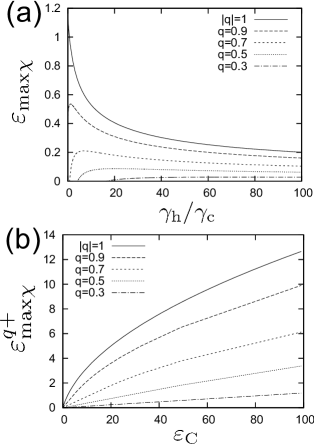
Figure 2: Numerical solutions for the nontight-coupling case $|q|\neq 1$: (a) Dependence of $\varepsilon_{\rm max\chi}$ on the dissipation ratio $\gamma_{\rm h}/\gamma_{\rm c}$ under given temperatures ($T_{\rm h}=1$ and $T_{\rm c}=0.7$) for some $q$’s. We also plot eq. (24) for the tight-coupling case $|q|=1$ for comparison. We always set $L_{11}=1$, $L_{22}=1$. Giving $q$, we can determine $L_{21}$ as $L_{21}=\sqrt{q^{2}L_{11}L_{22}}$. (b) Dependence of the upper bound $\varepsilon_{\rm max\chi}^{q+}$ on $\varepsilon_{\rm C}$ for some $q$’s. We also plot the upper bound $\varepsilon_{\rm max\chi}^{+}$ for the tight-coupling case $|q|=1$ in eq. (26) for comparison. We used the same values for $L_{ij}$’s as in (a). We fixed $T_{\rm h}=1$ and changed $T_{\rm c}$.

Comparing with the tight-coupling case, we found that the analytic solution of the nontight-coupling case becomes too complicated to write down explicitly. Thus we here solve the optimization problem numerically. We first note that eq. (20) implies the restriction

$$\gamma_{\rm c}<-\frac{L_{12}^{2}}{4(1-q^{2})L_{11}^{2}L_{22}X_{2}}\equiv\gamma_{\rm c}^{+},$$ (27)

for given Onsager coefficients $L_{ij}$’s and $X_{2}$. Such restriction does not appear in the tight-coupling case. Besides, we note that we also have the restriction $0<\gamma_{\rm c}<T_{\rm h}/L_{11}$ due to the assumption of the non-negativity of $\gamma_{\rm c}$ and $\gamma_{\rm h}$ as in eq. (14). Thus, by combining these two inequalities, we obtain the restriction of the dissipation ratio for the nontight-coupling case, depending on the value of $\gamma_{\rm c}^{+}$ as

$$0<\frac{\gamma_{\rm h}}{\gamma_{\rm c}}<\infty$$ (28)

in the case of ${T_{\rm h}}/{L_{11}}\leq\gamma_{\rm c}^{+}<\infty$, and

$$\frac{\frac{T_{\rm h}}{L_{11}}-\gamma_{\rm c}^{+}}{\gamma_{\rm c}^{+}}<\frac{\gamma_{\rm h}}{\gamma_{\rm c}}<\infty$$ (29)

in the case of $0<\gamma_{\rm c}^{+}<{T_{\rm h}}/{L_{11}}$, respectively.

We can obtain $\varepsilon_{\rm max\chi}$ numerically as follows: we fix the values of $L_{11}$, $L_{22}$, $q$, $T_{\rm h}$ and $T_{\rm c}$. Choosing $\gamma_{\rm c}$ so as to satisfy $0<\gamma_{\rm c}<T_{\rm h}/L_{11}$ and eq. (27), which also determines $\gamma_{\rm h}$ from eq. (14), we can find $\varepsilon$ at the maximum value of $\chi$ by calculating eq. (18) as $J_{1}$ is varied in the range of eq. (19).

We first consider typical dependence of $\varepsilon_{\rm max\chi}$ on the dissipation ratio $\gamma_{\rm h}/\gamma_{\rm c}$ under given temperatures for some $q$’s. By changing $\gamma_{\rm c}$, we plotted $\varepsilon_{\rm max\chi}$ as a function of $\gamma_{\rm h}/\gamma_{\rm c}$ in fig. 2 (a). As one of the interesting characteristics, we can see that the dependence can become non-monotonic and $\varepsilon_{\rm max\chi}$ attains the maximum value at a finite dissipation ratio for each $q$. This contrasts to the tight-coupling case in eq. (26), where its upper bound $\varepsilon_{\rm max\chi}^{+}$ is always attained in the asymmetric dissipation limit $\gamma_{\rm h}/\gamma_{\rm c}\to 0$.

Next we determine the upper bound $\varepsilon_{\rm max\chi}^{q+}$ and the lower bound $\varepsilon_{\rm max\chi}^{q-}$ for the nontight-coupling case under various temperatures. By changing $\varepsilon_{\rm C}$, we evaluated the maximum value of $\varepsilon_{\rm max\chi}$ as $\varepsilon_{\rm max\chi}^{q+}$ for some $q$’s (see fig. 2 (b)). We found that $\varepsilon_{\rm max\chi}^{q+}$ is always lower than $\varepsilon_{\rm max\chi}^{+}$ in eq. (26) and monotonically decreases as $q$ is decreased for each $\varepsilon_{\rm C}$. Meanwhile we also found that the lower bound $\varepsilon_{\rm max\chi}^{q-}$ agrees with $0$ for each $q$ (data not shown), which can always be attained in the asymmetric dissipation limit $\gamma_{\rm h}/\gamma_{\rm c}\to\infty$ as in the tight-coupling case in eq. (26). We also note that in the case where $\gamma_{\rm h}/\gamma_{\rm c}$ satisfies eq. (29), the lower bound $\varepsilon_{\rm max\chi}^{q-}=0$ can be realized also at the lower endpoint of eq. (29), that is, in the limit of $\gamma_{\rm h}/\gamma_{\rm c}\to(T_{\rm h}/L_{11}-\gamma_{\rm c}^{+})/\gamma_{\rm c}^{+}$. (See the lines of $q=0.3$, $0.5$ and $0.7$ in fig. 2 (a).) In this case, $\varepsilon_{\rm max\chi}^{q-}$ becomes $0$ since $J_{2}^{\rm max\chi}$ vanishes: in the lower endpoint of eq. (29), the discriminant $D$ in eq. (20) becomes $0$. Thus the solution of the inequality $J_{2}>0$ in eq. (19) approaches this multiple root in that limit, where $J_{2}$ in eq. (12) is identically $0$. This contrasts to the case of $\gamma_{\rm h}/\gamma_{\rm c}\to\infty$, where $J_{2}^{\rm max\chi}$ diverges.

3 Example: leaky low-dissipation Carnot refrigerator

As an example of the minimally nonlinear irreversible refrigerator, we here introduce a leaky low-dissipation Carnot refrigerator model. The original low-dissipation Carnot refrigerator without heat leak studied in [21, 26] is an extension of the quasistatic Carnot refrigerator by assuming that heat transfer accompanying finite-time operation in each isothermal process is inversely proportional to the duration of the process $t_{i}$:

$$Q_{\rm h}=T_{\rm h}\Delta S+\frac{T_{\rm h}\Sigma_{\rm h}}{t_{\rm h}},$$ (30)

$$Q_{\rm c}=T_{\rm c}\Delta S-\frac{T_{\rm c}\Sigma_{\rm c}}{t_{\rm c}},$$ (31)

where we denote by $\Delta S>0$ the quasistatic entropy change of the working system during each isothermal process, and by $\Sigma_{i}/t_{i}$ the corresponding entropy production with a constant strength $\Sigma_{i}>0$ [21, 26]. Then we formally modify this low-dissipation Carnot refrigerator to a leaky model by adding a heat leak term as follows:

$$Q_{\rm h}=T_{\rm h}\Delta S+\frac{T_{\rm h}\Sigma_{\rm h}}{t_{\rm h}}-\kappa(T_{\rm h}-T_{\rm c})(t_{\rm h}+t_{\rm c}),$$ (32)

$$Q_{\rm c}=T_{\rm c}\Delta S-\frac{T_{\rm c}\Sigma_{\rm c}}{t_{\rm c}}-\kappa(T_{\rm h}-T_{\rm c})(t_{\rm h}+t_{\rm c}),$$ (33)

where we assume the linear Fourier-type heat transfer from the hot heat reservoir to the cold one as the heat leak per cycle, denoting by $\kappa>0$ the effective thermal conductivity. We here reinterpret $Q_{\rm h}$ ($Q_{\rm c}$) as the net heat transfer into (from) the heat reservoir per cycle, instead of the heat transfer in each isothermal process, considering the heat leak contribution which always continues during one-cycle.

We show that this leaky low-dissipation Carnot refrigerator is an example of the minimally nonlinear irreversible refrigerator by rewriting eqs. (32) and (33) into the forms of eqs. (12) and (13): since it works as a cyclic refrigerator and according to eqs. (6) and (7), we can define its thermodynamic fluxes and forces as $J_{1}\equiv 1/t_{\rm cycle}=1/(t_{\rm h}+t_{\rm c})=1/((\alpha+1)t_{\rm h})$, $J_{2}\equiv\dot{Q}_{\rm c}=Q_{\rm c}/t_{\rm cycle}$, $X_{1}\equiv W/T_{\rm h}$ and $X_{2}\equiv 1/T_{\rm h}-1/T_{\rm c}$, with $\alpha\equiv t_{\rm c}/t_{\rm h}$. By using these definitions and eqs. (32) and (33), we can calculate the Onsager coefficients $L_{ij}$’s and the strength of the dissipation $\gamma_{i}$’s as

$$\left(\begin{array}[]{cc}L_{11}&L_{12}\\ L_{21}&L_{22}\end{array}\right)=\left(\begin{array}[]{cc}\frac{T_{\rm h}}{Y}&\frac{T_{\rm h}T_{\rm c}\Delta S}{Y}\\ \frac{T_{\rm h}T_{\rm c}\Delta S}{Y}&\frac{{T_{\rm c}^{2}{T_{\rm h}}{\Delta S}^{2}}}{Y}+T_{\rm h}T_{\rm c}\kappa\end{array}\right),$$ (38)

$$\gamma_{\rm h}=T_{\rm h}\Sigma_{\rm h}(\alpha+1),$$ (39)

$$\gamma_{\rm c}=\frac{T_{\rm c}\Sigma_{\rm c}(\alpha+1)}{\alpha},$$ (40)

respectively, where the common factor $Y$ in eq. (38) is given as

$$Y\equiv(\alpha+1)\left(T_{\rm h}\Sigma_{\rm h}+\frac{T_{\rm c}\Sigma_{\rm c}}{\alpha}\right).$$ (41)

From eq. (38) we see that the Onsager reciprocity $L_{12}=L_{21}$ holds as expected. In general, the Onsager coefficients show the nontight-coupling condition $|q|=\frac{L_{12}}{\sqrt{L_{11}L_{22}}}<1$, but recover the tight-coupling condition $|q|\to 1$ in the zero leak limit of $\kappa\to 0$. Thus our model eqs. (12) and (13) under the tight-coupling condition includes the low-dissipation Carnot refrigerator [21, 26] in eqs. (30) and (31) as a special case.

Finally we note that we obtained eq. (24) for the tight-coupling case maximizing $\chi$ only by one parameter $J_{1}$, whereas in the original low-dissipation model without the heat leak the optimization uses the two parameters $t_{\rm h}$ and $t_{\rm c}$ [21, 26]. Thus the parameter space for the maximization is different. In the formalism presented here, a further optimization of $\chi=\chi(\alpha)$ by $\alpha$ is still possible after the optimization by $J_{1}$ and it corresponds to the two-parameter maximization done in [21, 26]. But, that further optimization does not change the bounds in eq. (4). In particular, under symmetric conditions ($\Sigma_{\rm h}=\Sigma_{\rm c}$) the further optimization by $\alpha$ gives $\alpha_{\rm max\chi}=\sqrt{1-\tau}+1,$ from which we can straightforwardly obtain the symmetric optimization COP in eq. (3) [21].

4 Summary

We introduced the extended Onsager relations as the model of minimally nonlinear irreversible refrigerators, which can be applied to both steady-state and cyclic refrigerators. We analytically derived the general expression for the coefficient of performance (COP) under maximum $\chi$-condition when the tight-coupling condition is met and determined its upper and lower bounds which perfectly agree with the result derived previously in the low-dissipation Carnot refrigerator model in [26]. We also studied the nontight-coupling case numerically and found that its upper bound is always lower than that of the tight-coupling case, whereas all the cases have the same lower bound. Moreover, we introduce the leaky low-dissipation Carnot refrigerator. Calculating the Onsager coefficients and the strength of the power dissipation explicitly, we proved that this leaky low-dissipation Carnot refrigerator is an example of the minimally nonlinear irreversible refrigerator.

- [1] \NameEsposito M., Lindenberg K. Van den Broeck C. \REVIEWPhys. Rev. Lett.1022009130602.
- [2] \NameBenenti G., Saito K. Casati G. \REVIEWPhys. Rev. Lett.1062010060601.
- [3] \NameSánchez-Salas N., López-Palacios L., Velasco S. Calvo Hernández A. \REVIEWPhys. Rev. E822010051101.
- [4] \NameTu Z. C. \REVIEWChin. Phys. B212012020513.
- [5] \NameWu C., Chen L. Chen J. \BookAdvances in Finite-Time Thermodynamics: Analysis and Optimization \PublNova Science, New York \Year2004.
- [6] \NameDurmayaz A., Sogut O. S., Sahin B. Yavuz H. \REVIEWProg. Energy Combust. Sci.302004175.
- [7] \NameTu Z. C. \REVIEWJ. Phys. A: Math. Theor.412008312003.
- [8] \NameSchmiedl T. Seifert U. \REVIEWPhys. Rev. Lett.982007108301.
- [9] \NameSchmiedl T. Seifert U. \REVIEWEPL81200820003.
- [10] \NameSeifert U. \REVIEWPhys. Rev. Lett.1062011020601.
- [11] \NameGaveau B., Moreau M. Schulman L. S. \REVIEWPhys. Rev. Lett.1052011230602.
- [12] \NameEsposito M., Kawai R., Lindenberg K. Van den Broeck C. \REVIEWEPL89201020003.
- [13] \NameEsposito M., Kawai R., Lindenberg K. Van den Broeck C. \REVIEWPhys. Rev. E812010041106.
- [14] \NameAbe S. \REVIEWPhys. Rev. E832011041117.
- [15] \NameBlickle V. Bechinger C. \REVIEWNature Phys.82012143.
- [16] \NameCurzon F. Ahlborn B. \REVIEWAm. J. Phys.43197522.
- [17] \NameEsposito M., Kawai R., Lindenberg K. Van den Broeck C. \REVIEWPhys. Rev. Lett.1052010150603.
- [18] \NameYan H. Guo H. \REVIEWPhys. Rev. E852012011146.
- [19] \NameWang Y. Tu Z. C. \REVIEWPhys. Rev. E852012011127.
- [20] \NameWang Y. Tu. Z. C. \REVIEWEPL98201240001.
- [21] \Namede Tomás C., Calvo Hernández A. Roco J. M. M. \REVIEWPhys. Rev. E852012010104(R).
- [22] \NameYan Z. Chen J. \REVIEWJ. Phys. D231990136.
- [23] \NameVelasco S., Roco J. M. M., Medina A. Calvo Hernández A. \REVIEWPhys. Rev. Lett.7819973241.
- [24] \NameVelasco S., Roco J. M. M., Medina A. Calvo Hernández A. \REVIEWAppl. Phys. Lett.7119971130.
- [25] \NameAllahverdyan A. E., Hovhannisyan K. Mahler G. \REVIEWPhys. Rev. E812010051129.
- [26] \NameWang Y., Li M., Tu Z. C., Calvo Hernández A. Roco J. M. M. \REVIEWPhys. Rev. E862012011127.
- [27] \NameVan den Broeck C. \REVIEWPhys. Rev. Lett.952005190602.
- [28] \NameJiménez de Cisneros B., Arias-Hernández L. A. Calvo Hernández A. \REVIEWPhys. Rev. E732006057103.
- [29] \NameJiménez de Cisneros B. Calvo Hernández A. \REVIEWPhys. Rev. Lett.982007130602.
- [30] \NameJiménez de Cisneros B. Calvo Hernández A. \REVIEWPhys. Rev. E772008041127.
- [31] \NameIzumida Y. Okuda K. \REVIEWPhys. Rev. E802009021121.
- [32] \NameIzumida Y. Okuda K. \REVIEWEur. Phys. J. B.772010499.
- [33] \NameIzumida Y. Okuda K. \REVIEWEPL83200860003.
- [34] \NameIzumida Y. Okuda K. \REVIEWEPL97201210004.
- [35] \NameOnsager L. \REVIEWPhys. Rev.371931405.
- [36] \Namede Groot S. R. Mazur P. \BookNon-Equilibrium Thermodynamics \PublDover, New York \Year1984.
- [37] \NameCallen H. B. Welton T. A. \REVIEWPhys. Rev.83195134.
- [38] \NameApertet Y., Ouerdane H., Glavatskaya O., Goupil C. Lecoeur Ph. \REVIEWEPL97201228001.
- [39] \NameApertet Y., Ouerdane H., Goupil C. Lecoeur Ph. \REVIEWPhys. Rev. E852012041144.