Gibbsian Method for the Self-Optimization of Cellular Networks

Abstract

In this work, we propose and analyze a class of distributed algorithms performing the joint optimization of radio resources in heterogeneous cellular networks made of a juxtaposition of macro and small cells. Within this context, it is essential to use algorithms able to simultaneously solve the problems of channel selection, user association and power control. In such networks, the unpredictability of the cell and user patterns also requires distributed optimization schemes. The proposed method is inspired from statistical physics and based on the Gibbs sampler. It does not require the concavity/convexity, monotonicity or duality properties common to classical optimization problems. Besides, it supports discrete optimization which is especially useful to practical systems. We show that it can be implemented in a fully distributed way and nevertheless achieves system-wide optimality. We use simulation to compare this solution to today’s default operational methods in terms of both throughput and energy consumption. Finally, we address concrete issues for the implementation of this solution and analyze the overhead traffic required within the framework of 3GPP and femtocell standards.

1 Introduction

Today’s cellular mobile radio systems strongly rely on highly hierarchical network architectures that allow service providers to control and share radio resources among base stations and clients in a centralized manner. With the foreseen exponentially increasing number of users and traffic in the 4G and future wireless networks, existing deployment and practice becomes economically unsustainable. Network self-organization and self-optimization are among the key targets of future mobile networks so as to relax the heavy demand of human efforts in the network planning and optimization tasks and to reduce the system’s capital and operational expenditure (CAPEX/OPEX) [1, 2, 3]. The next-generation mobile networks (NGMN) are expected to provide a full coverage of broadband wireless service and support fair and efficient radio resource utilization with a high degree of operation autonomy and intelligence.

Due to the emerging high demand of broadband service and new applications, wireless networking also has to face the challenge of supporting fast increasing data traffic with the requirement of spectrum and energy utilization efficiency [4]. To enhance the network capacity and support pervasive broadband service, reducing cell size is one of the most effective approaches. Deployment of small cell base stations or femtocells has a great potential to improve the spatial reuse of radio resource and also enhance transmit power efficiency [5]. It is foreseen that the next generation of mobile cellular networks will consist of heterogeneous macro and small cells with different capabilities including transmit power and coverage range. In such networks due to the unpredictability of the base station and user patterns, network self-organization and self-optimization become necessary. Autonomic management and configuration of user association, i.e., assigning users to base stations, and radio resource allocation such as transmit power and channel selection would be highly desirable to practical systems [6].

The primary objective of the present work is to design distributed algorithms performing radio resource allocation and network self-optimization for today’s macro and small cell (e.g., 3GPP-LTE [2] and femtocell) mixed networks. In radio resource management, (i) power control, (ii) user association and (iii) channel selection are essential elements. It is known that system-wide radio resource optimization is usually very challenging [7]. A joint optimization of user association, channel selection and power control is in general non-convex and difficult to solve, even if centralized algorithms are allowed [8]. Notice that in classical networks made of macro cells only, optimizing any of the above three elements independently can effectively improve the system performance. However, this may not be true in heterogeneous networks made of a juxtaposition of macro and small cells. This would yield extra complexity and difficulties. Besides, future wireless networks will typically be large, have fairly random topologies, and lack centralized control entities for allocating resources and explicitly coordinating transmissions with global coordination. Instead, these networks will depend on individual nodes to operate autonomously and iteratively and to share radio resources efficiently. We have to see how individual nodes can perform autonomously and support inter-cell interference management in a distributed way for finding globally optimal configurations.

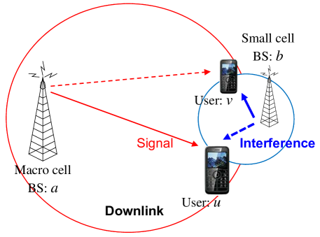
Figure 1: Since user $u$ is far from its BS $a$, the received signal at user $u$ may suffer strong interference due to the transmission of small cell BS $b$ destined to user $v$.

To begin with, we give two examples to illustrate the problems that may happen when conducting these optimizations under macro and small cell networks, in both the downlink and uplink respectively. Consider the downlink scenario in Figure 1 where there are two mobile users $u$ and $v$ under the macro and small cell base stations (BS) $a$ and $b$ which have different maximum transmit powers and coverage ranges. Notice that user $u$ can be covered by the macro cell BS $a$ but it is located near the edge of $a$’s coverage. Meanwhile, it is too close to the small cell BS $b$ and this will have a strong impact on its received signal-to-interference-plus-noise-ratio (SINR). Here, transmit power optimization will not be effective without prior user association and channel selection optimization. One may consider the option in which users $u$ and $v$ both associate with the small cell $b$. However, this may overload BS $b$. From the viewpoint of load balancing, it is better to have the two users attached to different cells, e.g., user $u$ is attached to BS $a$. However, user $u$ will then have a low SINR as long as the two transmissions use a same channel. Clearly, one should consider assigning two different channels for these two transmitter-receiver pairs and hence conduct a joint user association and channel selection optimization with respect to the link characteristics of the possible combinations and their available channels. If the system involves more users and cells, power control should be conducted as well to mitigate interference. This requires a joint optimization of all three elements.

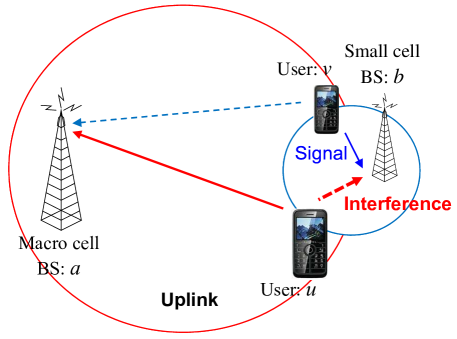
Figure 2: The signal received at BS $b$ sent from user $v$ can be strongly interfered by the transmission of user $u$ since $u$ has to use a relatively high power in order to send its signal to BS $a$ in long distance.

Figure 2 shows a similar problem in the uplink. Consider that one first conducts user association optimization. Since user $v$ is closer to BS $b$ than to BS $a$, from the viewpoint of load balancing, the recommended user association should be as follows: user $u$ attaches to BS $a$ while user $v$ attaches to BS $b$. As user $u$ is far away from its BS $a$, the transmit power has to be high enough. This will however yield a strong interference to the signal received at BS $b$ which is transmitted from user $v$. Note that in this case, user association optimization, power control or even their joint optimization are not able to solve the problem. However, if one also considers channel allocation and tries to select two different channels for these two transmitter-receiver pairs, a joint optimization will be able to resolve the conflict and enhance overall performance.

Let us now describe what aspects of the problem were considered so far and the novelty of our approach. When each optimization is conducted separately, the proper optimization sequence was studied in [9, 10] for the 802.11 WLAN case, based on careful experimental work and scenario analysis. Explicit rules were proposed when the cell patterns have a specific structure (e.g., in the hexagonal base station pattern case). However, for situations where the cell and user patterns are unpredictable as in the small cell case, no simple and universal rule is known and a joint optimization is necessary to achieve the best performance.

Various separate optimization problems were considered, mainly under the assumptions of centralized coordination and global information exchange. For example the transmission powers maximizing system throughput in the multiple interfering link case leads to a non-convex optimization problem which was studied in [11, 12]. A power control algorithm that guarantees strict throughput maximization in the general SINR regime is reported in [13]. It is built on multiplicative linear fractional programming, which is used for optimization problems expressible as a difference of two convex problems. However, this algorithm requires a centralized control and is only efficient for problem instances of small size due to the computation complexity. There is a lack of efficient algorithm operating in a distributed manner and ensuring global optimality in the above joint optimization.

Here, we propose and analyze a class of distributed algorithms performing the joint optimization of radio resources in a generalized heterogeneous macro and small cell network. Note that the optimization function does not have qualitative properties such as convexity or monotonicity. The proposed solution is inspired from statistical physics and based on the Gibbs sampler (see e.g., [14, 15]). It is a generalization of the work in [3] which only takes into account power control and user association and is thus limited to homogeneous mobile cellular networks. The paper describes the algorithm, shows that the latter can be implemented in a fully distributed manner and nevertheless achieves minimal system-wide potential delay, reports on its performance, and analyzes the overhead associated with the information exchange required in the implementation of this solution in today’s 3GPP-LTE and femtocell standards. The rest of the paper is organized as follows. Section 2 describes the system model and problem setup. Section 3 presents the proposed solution. Section 4 compares this solution to today’s default operation in terms of throughput and energy consumption. Section 5 investigates the overhead traffic generated by the algorithm. Finally, Section 6 contains the conclusion.

2 System Model and Problem Formulation

We consider a reuse-1 cellular radio system with a set $\mathcal{B}$ of base stations serving a population $\mathcal{U}$ of users. For each user $u\in\mathcal{U}$, it is assumed that there is a pair of orthogonal channels for the uplink and downlink. We assume that there is no interference between the uplink and downlink and we only consider the downlink. However, the method can be generalized to the uplink as well.

We assume that users can associate with any neighboring base station $b\in\mathcal{B}$ in the network which could be a macro or small cell base station, which is referred to as open access [5]. Today’s default operation attaches each user $u$ to the base station with the highest received power. Note that this is clearly sub-optimal. In general, if one simply associates users with the closest BS or to that with the strongest received signal, it is possible that some BSs have many users while others have only a few. The resulting overload might lead to a degradation of the network capacity.

Let $\mathcal{C}$ be the set of channels (e.g., frequency bands) which are common to all base stations. The base station serving user $u$ is denoted by $b_{u}$ and is restricted to some local set ${\mathcal{B}}_{u}$ of bases stations (typically ${\mathcal{B}}_{u}$ is the set of BSs the power of pilot signal of which is received by user $u$ above some threshold). The channel allocated by $b_{u}$ to user $u$ is denoted $c_{u}\in\mathcal{C}$. Here, for simplicity we consider that a user only takes one channel. The transmission power used by base station $b_{u}$ to $u$ is denoted by $P_{u}$.

The SINR at user $u$ is then:

$$\textrm{{sinr}}_{u}=\frac{P_{u}l(b_{u},u,c_{u})}{N_{u}(c_{u})+\sum\limits_{v\in\mathcal{U},v\neq u}\alpha(b_{u},b_{v},c_{u},c_{v})P_{v}l(b_{v},u,c_{v})}~{},$$ (1)

where $N_{u}(c)$ denotes the thermal noise of user $u$ on channel $c$, $l(b_{u},u,c)$ is the signal attenuation from BS $b_{u}$ to $u$ on channel $c$, and $\alpha(b,b^{\prime},c,c^{\prime})$ represents the orthogonality factor between some user associated with BS $b$ on channel $c$ and some user associated with BS $b^{\prime}$ on channel $c^{\prime}$.

Note that it makes sense to assume that $0\leq\alpha(\cdot)\leq 1$ and that the following symmetry holds: for all $b,b^{\prime},c,c^{\prime}$,

$$\alpha(b,b^{\prime},c,c^{\prime})=\alpha(b^{\prime},b,c^{\prime},c).$$

Here are some examples: if adjacent channel interference is negligible compared to co-channel interference, then one should take $\alpha(b,b^{\prime},c,c^{\prime})=0$ for $c\neq c^{\prime}$. One may also assume that $\alpha(b,b,c,c)=\alpha$ and $\alpha(b,b^{\prime},c,c)=\beta$ for $b\neq b^{\prime}$, where $\alpha$ and $\beta$ are some constants such that $\alpha<\beta$. The simplest case is that where $\alpha=\beta=1$.

Under the additive white Gaussian noise (AWGN) model, the achievable data rate at user $u$ in bit/s/Hz is given by:

$$r_{u}=K\log(1+\textrm{{sinr}}_{u})~{},$$ (2)

where $K$ is a constant depending on the width of the frequency band.

To achieve network throughput enhancement while supporting bandwidth sharing fairness among users, we adopt the notion of minimal potential delay fairness proposed in [16]. This solution for bandwidth sharing is intermediate between max-min and proportional fairness. It aims at minimizing the system-wide potential delay and is explained below.

Instead of maximizing the sum of throughputs, i.e., $\sum r_{u}$, which often leads to very low throughput for some users, we minimize the sum of the inverse of throughput, i.e., $\sum r_{u}^{-1}$, which can be seen as the total delay spent to send an information unit to all the users. Note that minimizing $\sum r_{u}^{-1}$ penalizes very low throughputs. More explicitly, a bandwidth allocation that provides minimal potential delay fairness is one that minimizes the following cost function:

$$C=\sum_{u\in\mathcal{U}}\frac{1}{r_{u}}~{},$$ (3)

which is the network’s aggregate transmission delay. It also indicates the long term throughput that a user expects to receive from a fully saturated network.

For mathematical convenience (see below), in this paper, we minimize the cost function

$$\mathcal{E}=\sum_{u\in\mathcal{U}}\frac{1}{e^{\frac{r_{u}}{K}}-1}=\sum_{u\in\mathcal{U}}\frac{1}{\textrm{{sinr}}_{u}}$$ (4)

instead of (3). We call $\mathcal{E}$ the global energy, following the terminology of Gibbs sampling. Note that if one operates in a low SINR regime such that the achievable data rate of a user is proportional to its SINR, e.g., $r_{u}=K\textrm{{sinr}}_{u}$, minimizing the potential delay $C$ is equivalent to minimizing the global energy $\mathcal{E}$.

Remark 1

$\mathcal{E}$ is a surrogate of $C$. We see that (3) and (4) have quite similar characteristics. The difference is that $(e^{\frac{r_{u}}{K}}-1)^{-1}$ increases more significantly than $r_{u}^{-1}$ when $r_{u}$ is low. As a result, the overall cost will increase more substantially. So, minimizing $\mathcal{E}$ rather than $C$ penalizes low throughputs more significantly and favors a higher level of user fairness.

By (1) and (2), the global energy $\mathcal{E}$ in (4) can be written as:

$$\mathcal{E}=\sum_{u\in\mathcal{U}}\frac{N_{u}(c_{u})+\sum\limits_{v\in\mathcal{U},v\neq u}\alpha(b_{u},b_{v},c_{u},c_{v})P_{v}l(b_{v},u,c_{v})}{P_{u}l(b_{u},u,c_{u})}$$ (5)

so that

$$\mathcal{E}=\sum_{u\in\mathcal{U}}\frac{N_{u}(c_{u})}{P_{u}l(b_{u},u,c_{u})}+~{}~{}~{}~{}~{}~{}~{}~{}~{}~{}~{}~{}~{}~{}~{}~{}~{}~{}~{}~{}~{}~{}~{}~{}~{}~{}~{}~{}~{}~{}~{}~{}~{}~{}~{}~{}~{}~{}~{}~{}~{}~{}~{}~{}~{}~{}~{}~{}~{}~{}~{}~{}~{}~{}~{}~{}~{}~{}$$

$$\sum_{\{u,v\}\subseteq\mathcal{U}}\left(\frac{\alpha(b_{u},b_{v},c_{u},c_{v})P_{v}l(b_{v},u,c_{v})}{P_{u}l(b_{u},u,c_{u})}+\right.\left.\frac{\alpha(b_{v},b_{u},c_{v},c_{u})P_{u}l(b_{u},v,c_{u})}{P_{v}l(b_{v},v,c_{v})}\right).$$ (6)

The optimization problem consists in finding a configuration (also referred to as a state) of user association, channel selection and power allocation which minimizes the above energy function. It is clear that the problem has a high combinatorial complexity and is in general hard to solve for large networks. However the additive structure of the energy can be used to conduct its minimization using a Gibbs sampler. This leverages the decomposition of $\mathcal{E}$ into a sum of local cost function for each user $u$ (say local energy $\mathcal{E}_{u}$) which can be manipulated in a distributed way in the resource allocation. We explain this setup and optimization in the next section.

3 Gibbs Sampler and Self Optimization

We now describe the distributed algorithm to perform the joint optimization of user association, channel selection and power control. It is based on a Gibbs sampler operating on a graph $\mathcal{G}$ of the network which can be defined as follows:

• The set of nodes in $\mathcal{G}$ is the set of users denoted by $u\in\mathcal{U}$.

• Each node $u$ is endowed with a state variable $s_{u}$ belonging to a finite set $\mathcal{S}$. The state of a node is a triple describing its user association, its channel and its transmit power; this state denoted by $s_{u}=\{b_{u},c_{u},P_{u}\}$. Here, we consider that transmit power is discretized. We denote the state of the graph by $\mathbf{s}\triangleq(s_{u})_{u\in\mathcal{U}}$.

• Two user nodes $u$ and $v$ are neighbors in this graph if either (i) the power $P_{0}$ of the pilot signal received from a possible association base station for $v$ at $u$ is above some threshold, say $\theta$ or (ii) the power received from a possible base station for $u$ is above $\theta$ at $v$. We denote the set of neighbors of $u$ by $\mathcal{N}_{u}$. Notice that $v\in\mathcal{N}_{u}$ if and only if $u\in\mathcal{N}_{v}$.

Below, for all subsets $\mathcal{V}\subseteq\mathcal{U}$, the cardinality of $\mathcal{V}$ is denoted by $|\mathcal{V}|$.

The global energy $\mathcal{E}=\mathcal{E}({\mathbf{s}})$ in (2) derives from a potential function $V(\mathcal{V})$ [15], that is

$$\mathcal{E}=\sum_{\mathcal{V}\subseteq\mathcal{U}}V(\mathcal{V}),$$ (7)

where the sum bears on the set of all cliques of the graph defined above and where the potential function $V(\cdot)$ has here the following form:

$$\left\{\begin{array}[]{rll}V(\mathcal{V})&=\displaystyle\frac{N_{u}(c_{u})}{P_{u}l(b_{u},u,c_{u})}&\;\textrm{ if }\;\mathcal{V}=\{u\},\vspace{0.15cm}\\ V(\mathcal{V})&=\displaystyle\frac{\alpha(b_{u},b_{v},c_{u},c_{v})P_{v}l(b_{v},u,c_{v})}{P_{u}l(b_{u},u,c_{u})}+\frac{\alpha(b_{v},b_{u},c_{v},c_{u})P_{u}l(b_{u},v,c_{u})}{P_{v}l(b_{v},v,c_{v})}\;\textrm{ ~{}~{}if }\;\mathcal{V}=\{u,v\},\vspace{0.15cm}\\ \vspace{0.15cm}V(\mathcal{V})&=\displaystyle 0&\;\textrm{ if }\;|\mathcal{V}|\geq 3.\end{array}\right.$$

A global energy which derives from such a potential function satisfying the condition $V(\mathcal{V})=0$ for $|\mathcal{V}|\geq 3$ is hence amenable to a distributed optimization using the Gibbs sampler, which is based on the evaluation of the local energy at each node:

$$\mathcal{E}_{u}=\sum_{\mathcal{V}\subseteq\mathcal{U}\ s.t.\ u\in\mathcal{V}}V(\mathcal{V})~{}.$$ (8)

Following the above definition of $V(\cdot)$, this can be re-written as:

$$\mathcal{E}_{u}({\mathbf{s}})=\underbrace{\frac{N_{u}(c_{u})+\sum\limits_{v\neq u,v\in{\cal N}_{u}}\alpha(b_{u},b_{v},c_{u},c_{v})P_{v}l(b_{v},u,c_{v})}{P_{u}l(b_{u},u,c_{u})}}_{=1/(\textrm{{sinr}}_{u})}+\sum_{v\neq u,v\in{\cal N}_{u}}\frac{\alpha(b_{v},b_{u},c_{v},c_{u})P_{u}l(b_{u},v,c_{u})}{P_{v}l(b_{v},v,c_{v})}~{}.$$ (9)

The local energy can be written in the following form:

$$\mathcal{E}_{u}(\mathbf{s})=A_{u}(\mathbf{s})+B_{u}(\mathbf{s}),$$ (10)

where $A_{u}(\mathbf{s})$ and $B_{u}(\mathbf{s})$ represent the first and second terms of (9), respectively. Notice that the first term $A_{u}(\mathbf{s})$ is equal to $1/\textrm{{sinr}}_{u}$. It is the “selfish” part of the energy function, which is small when $\textrm{{sinr}}_{u}$ is large. On the other hand, $B_{u}(\mathbf{s})$ is the “altruistic” part of the energy, which is small when the power of the interference incurred by all the other users because of $u$ is small compared to the power received from their own base stations.

Remark 2

One can consider that $\mathcal{E}_{u}$ consists of an individual cost of $u$ plus another term which corresponds to its impact on the others ($v\neq u$).

Remark 3

The above formulation is meant to handle joint power, channel, and user association optimization. However, it can easily be adapted to some special cases, e.g., to the case where the transmit power is a constant.

In the following, we describe more precisely the Gibbs sampler and its properties. First, we explain what it does. Each BS separately triggers a state transition for one of its users picked at random, say $u$, using a local random timer. This transition is selected based on the local energy $\mathcal{E}_{u}$. More precisely, given the state $(s_{v})_{v\neq u,\ v\in{\cal N}_{u}}$ of the neighbors of $u$, the new state $s_{u}$ is selected in the set ${\mathcal{S}}_{u}$ of potential states for user $u$ (this set is finite as power has been quantized to a finite set) with the probability

$$\pi_{u}(s_{u})=\frac{e^{-\frac{\mathcal{E}_{u}(s_{u},(s_{v})_{v\in\mathcal{N}_{u}})}{T}}}{\sum\limits_{s\in\mathcal{S}_{u}}e^{-\frac{\mathcal{E}_{u}(s,(s_{v})_{v\in\mathcal{N}_{u}})}{T}}}~{},~{}~{}s_{u}\in\mathcal{S}_{u}~{},$$ (11)

where $T>0$ is a parameter called the temperature.

We now list the properties of this sampler.

• These local random transitions drive the network to a steady state which is the Gibbs distribution associated with the global energy and temperature $T$, that is to a state with the following distribution (in steady state):

  $$\pi_{T}(\mathbf{s})=c\cdot e^{-\mathcal{E}(\mathbf{s})/T},$$

  with $c$ a normalizing constant. The proof is based on a reversibility argument similar to that of [15].

• This distribution puts more mass on low energy (small cost) configurations and when $T\rightarrow 0$, the distribution $\pi_{T}(\cdot)$ converges to a Dirac mass at the state of minimal cost if it is unique (otherwise to a uniform distribution on the minima).

• This procedure is distributed in that the transition of user $u$ only requires knowledge of the state of its neighbors. We discuss the structure of message exchanges in more detail below.

The exact procedure which users follow to conduct state transitions is summarized in Algorithm 1. Each user sets a timer, $t_{u}$, which decreases linearly with time. We consider discrete time in step of $\delta$ second(s) and simply set $\delta=1$. This timer has a duration randomly sampled according to a geometric distribution. When $t_{u}$ expires, a transition of $u$ occurs by which the state of this user is updated as indicated above.

every $\delta$ do  foreach $u$ do  if $t_{u}\leq 0$ then  forall $s$ in $\mathcal{S}_{u}$ do  $\displaystyle\mathcal{E}_{u}(s,(s_{v},v\neq u))\leftarrow A_{u}(s,(s_{v},v\neq u))+B_{u}(s,(s_{v},v\neq u))$;

$d_{u}(s,(s_{v},v\neq u))\leftarrow\exp\left(-\mathcal{E}_{u}(s,(s_{v},v\neq u))/T\right)$;

end sample $s_{u}\in\mathcal{S}$ according to the probability law $\pi_{u}(s,(s_{v},v\neq u))\triangleq d_{u}(s_{u})/\sum_{s\in\mathcal{S}_{u}}d_{u}(s,(s_{v},v\neq u))$;

sample $t_{u}\geq 0$ with distribution $geom(1)$;

else  $t_{u}\leftarrow t_{u}-\delta$;

end end end

Algorithm 1 State transition for the Gibbs sampler.

3.1 A Few Remarks

Greedy Variant

One may consider to perform the state transition by deterministically choosing the one that maximizes (11) namely the best response instead of selecting a state according to the Gibbsian probability distribution. It is known that a strategy of best response will drive the system to a local minimum but not necessarily to an optimal solution. Some discussions on the price of anarchy of a best response algorithm can be found in [17] and references therein. The basic idea of the probabilistic approach described above is to keep a possibility to escape from being trapped in a local minimum.

Temperature and Speed of Convergence

It is clear that the tuning of the temperature $T$ will strongly impact the system’s limiting distribution. It has to be chosen by taking the tradeoff between the convergence speed and the strict optimality of the limit distribution into account.

It is known that under conditions which ensure the compactness of the Markov forward operator and the irreducibility of the corresponding chain [18], the Gibbs sampler will converge geometrically fast (for $T$ fixed) to the Gibbs distribution. In Section 4, we will present simulation results illustrating this convergence.

Annealed Variant

For a fixed environment (i.e., user population, signal attenuation), if one decreases $T$ as $T=1/\ln(1+t)$, where $t$ is time, then the algorithm will drive the network to a state of minimal energy, starting from any state. A concrete proof of this result is similar to that of [15, pp. 311-313]. This proof is based on the notion of weak ergodicity of Markov chains and reversibility argument and is omitted.

3.2 Message Exchanges

Two base stations, say $b$ and $b^{\prime}$, are called implicit neighbors if there exist two neighboring users $u$ and $u^{\prime}$ such that $u$ can associate to $b$ and $u^{\prime}$ to $b^{\prime}$, i.e., if $b\in{\mathcal{B}}_{u}$, $b^{\prime}\in{\mathcal{B}}_{u^{\prime}}$, and either $\alpha(b,b^{\prime},c,c^{\prime})P_{0}l(b^{\prime},u,c^{\prime})>\theta$ or $\alpha(b,b^{\prime},c,c^{\prime})P_{0}l(b,u^{\prime},c)>\theta$ for some $c$, $c^{\prime}$. As we shall see, messages have to be exchanged between implicit neighbor base stations only (in addition to those between users and their current association base station).

The necessity for message exchange comes from the need of sampling $s_{u}$ in the algorithm. For this either user $u$ or its base station $\hat{b}_{u}$ before the sampling (below we assume that the sampling takes place on $\hat{b}_{u}$) has to have enough information to determine $\pi_{u}({s,(s_{v},v\neq u)})$ or equivalently $\mathcal{E}_{u}(s,(s_{v},v\neq u))$ for all $s\in{\mathcal{S}}_{u}$. For this, some measurements and information exchange between neighboring base stations and users are required.

The explicit definition of $\mathcal{E}_{u}$ in (9), shows that for the evaluation of $A_{u}(s)$, a user $u$ will have to estimate the following data and report them to its base station $\hat{b}_{u}$:

1. the receiver noise: $N_{u}(c)$ on each channel $c$,

2. the total received interferences: $\sum_{v\neq u}\alpha(b,b_{v},c,c_{v})P_{v}l(b_{v},u,c)$, for each $c$ and for each $b\in{\mathcal{B}}_{u}$, and

3. the path-loss or link gain: $l(b,u,c)$, for each $c$ and for each $b$ in the set ${\mathcal{B}}_{u}$.

In order for $u$ or $\hat{b}_{u}$ to evaluate $B_{u}(s)$, for all $s\in{\mathcal{S}}_{u}$, each user $v\in{\cal N}_{u}$ will have to estimate the following information and to report to its own base station $b_{v}$ (which will in turn communicate it to all its implicit neighbors including $b_{u}$ on the backhaul network):

1. the power of its received signal: $P_{v}l(b_{v},v,c_{v})$, and

2. the path-loss or link gain: $\alpha(b_{v},b,c_{v},c)l(b,v,c)$, for each $c$ and for each of $b\in{\mathcal{B}}_{u}$.

Note that the measurement of signal power, interference and path-loss $l(b,u,c)$ for each considered channel from either its own base station or neighboring base stations can be retrieved by the user terminal from for example the measurement of available RSCP (received signal code power) and/or RSSI (received signal strength indication).

By the above information exchange, for each $u$, base station $\hat{b}_{u}$ is able to compute $\mathcal{E}_{u}$ for all $s\in{\mathcal{S}}_{u}$ and hence to sample the new state $s_{u}$ of user $u$ according to the above algorithm. Notice that inter-cell communication takes place between implicit neighbor base stations only. There is no need to transmit this information via the wireless medium. We assume that this is supported by the backhaul network. The amount of overhead traffic generated by the algorithm can be evaluated. The results on the matter are presented in Section 5.

4 Simulation and Comparison

A performance investigation of the proposed solution is conducted below. We implement Algorithm 1 and compare its performance with today’s 3GPP default operations [19] by discrete event simulations.

In the current standard and 3G implementations, base stations are usually configured with a nominal fixed transmission power such that the pilot signal can be received by terminals over the covered area. The downlink transmit power is often the maximum allowable power as well for a better user reception and coverage. Note that the pilot signal is broadcasted continuously to allow user equipments (UE) to perform channel measurements and appropriate tuning. In user association, the current practice consists in attaching a user to the BS received with the strongest signal strength (rather than the nearest base station). Note that this could lead to attaching the users to a far macro cell BS which has a higher transmit power than that of a nearer small cell BS. This is in general sub-optimal. In channel allocation, the current practice often follows a heuristic scheme where channels of a BS are assigned to its users simply in a round-robin fashion, i.e., sequentially, and in such a way that the numbers of users on each channels are well balanced and almost equal.

In the simulations, we consider that mobile users are uniformly distributed in a geographic area of $1000$ meters times $650$ meters and we adopt the 3GPP-3GPP2 spatial channel model [20]. The distance dependent path-loss is given by:

$$l^{\textrm{(dB)}}(d)=-30.18-26\log_{10}(d)-X_{\sigma}^{\textrm{(dB)}}~{},$$ (12)

where $d$ is the transmitter-receiver distance and $X_{\sigma}$ refers to log-normal shadowing with zero mean and standard deviation 4 dB. With operating temperature 290 Kelvin and bandwidth 1 MHz, the thermal noise $N_{u}$ is equal to $4.0039\times 10^{-15}$ W, for all $u$.

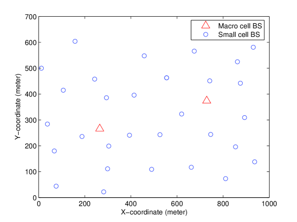
Figure 3: The geographic location of macro and small cell base stations (example).

Here we consider that there are two macro cell base stations with fixed locations as shown in Figure 3 and a number of small cell base stations which are randomly located in the geographical area. The maximum transmit power of macro and small cell base stations are 40W and 1W respectively. We assume that $P_{\delta}=0.1$ W. In the simulation, we consider a simple system where $\alpha=1$ and each user only takes one channel.

4.1 Numerical Examples

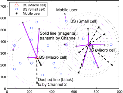
(a) Example 1: i) 8.7 b/s/Hz, ii) 0.012 b/s/Hz/W                                  

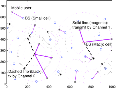
(b) Example 2: i) 35 b/s/Hz, ii) 0.106 b/s/Hz/W

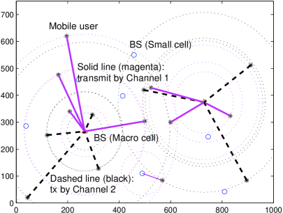
(c) Example 3: i) 7.5 b/s/Hz, ii) 0.009 b/s/Hz/W

Figure 4: Network before optimization (default operation). (a) Example 1: users are concentrated and fewer than BS. (b) Example 2: users are distributed and fewer than BS. (c) Example 3: more users than BS. Performance measure: i) system throughput, and ii) power efficiency. There are two orthogonal channels represented by solid-magenta and dashed-black lines.

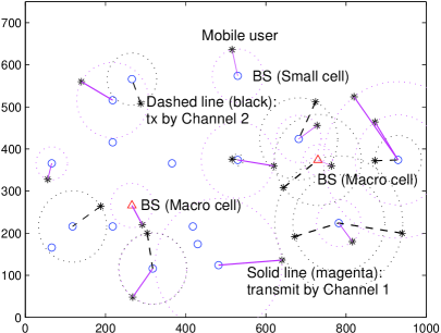
(a) Example 1: i) 43.5 b/s/Hz, ii) 3.45 b/s/Hz/W                                  

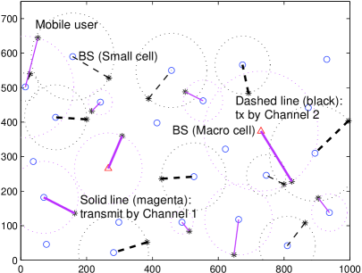
(b) Example 2: i) 75 b/s/Hz, ii) 4.41 b/s/Hz/W

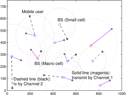
(c) Example 3: i) 32 b/s/Hz, ii) 2.13 b/s/Hz/W

Figure 5: Network after proposed joint optimization. Both the system throughput (b/s/Hz) and power utilization efficiency (b/s/Hz/W) are significantly improved.

To begin with, we illustrate the effectiveness of the algorithm by some examples with randomly generated small cell BS and users, as shown in Figures 4–5. To have readable graphical representation and comparison of the user association, channel allocation and transmission power before and after optimization, in these examples, we consider that the path-loss is simply distance dependent without log-normal shadowing. So, a user who is farther from a BS has a larger path-loss due to the larger distance. A line connecting a BS and a user indicates the user association and its thickness represents the strength of the transmit power. In these examples, we consider that there are two orthogonal channels in each BS, which are represented by different colors and line styles.

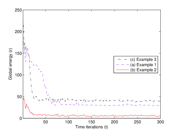
Figure 6: Convergence of the algorithm: (a) Example 1, (b) Example 2, and (c) Example 3, respectively.

Our simulations show that the proposed solution significantly outperforms the by-default configuration in both system throughput (in b/s/Hz) and power consumption efficiency (in b/s/Hz/W). Note that the latter has been improved by several orders of magnitude (also because our representation of the default operation has no power control mechanism). Figure 6 shows the corresponding convergence of the algorithm in the above three examples. We see that the algorithm usually converges in a few hundreds of iterations and is hence practical.

4.2 Average Performance

Secondly, we compare the performance of the proposed optimization with the default operation, with a fixed number of 32 BS (including the two macro BS) but with different numbers of users (denoted by $M$), i.e., different user densities, and different numbers of orthogonal channels (denoted by $K$). Users and small cells are randomly generated in the geographical area. For each $(M,K)$, 500 different topologies are sampled and the performance metrics are then averaged out.

Table 1 shows the the enhancement of the system throughput and of the power efficiency obtained by the joint optimization. Observe that for a given $M/K$ ratio, the spectrum utilization efficiency that results from the optimization increases with $K$. This observation is important for e.g., in 3GPP HSDPA (High Speed Downlink Packet Access) and LTE, where a high number of users and a high number of resources are typical.

5 Evaluation of Overhead Traffic

The aim of this Section is to evaluate the overhead traffic generated by the algorithms in a specific scenario which is based on the assumption that nodes form realizations of Poisson point processes in the Euclidean plane. These assumptions allow us to use elementary stochastic geometry to get estimates of this overhead traffic.

We concentrate on the channel selection and power control optimization, when assuming that users are associated with their closest or best base station. The overhead traffic has two main components: (i) the uplink radio traffic and (ii) the backhaul traffic.

5.1 Setting

The uplink radio overhead traffic is comprised of the set of messages that are sent by each mobile to its serving base station and that inform the latter of the path-loss that it experiences from each of its neighboring base stations. These data are required to run the algorithm, see e.g., (9). If one denotes by $\tau$ the frequency of the beaconing signals from the base stations and if one assumes that the users report their path-loss variables at each beacon, each mobile has to report $N\times\tau$ path-loss per second when the number of its neighboring base stations is $N$.

On the other hand, the backhaul traffic is between base stations (it is typically transported by a wireline infrastructure). We will say here that two base stations are neighbors if one of them has customers which see the other as a neighboring base station.

Consider a pair of neighboring base stations. Let $M_{1}$ denote the number customers of the first base station (say BS 1) which see the second (say BS 2) as a neighboring base station. Let $M_{2}$ be the symmetrical variable. Then the global backhaul traffic between the two stations is given by:

$$\sum_{i=1}^{M_{1}}\tau N_{1,i}+\sum_{j=1}^{M_{2}}\tau N_{2,j}$$ (13)

where $N_{1,i}$ denotes the number of neighboring base stations of BS 1 for user $i$ and $N_{2,j}$ denotes the number of neighboring base stations of BS 2 for user $j$. Note that their definitions are symmetric.

5.2 Stochastic Geometry Model

We first describe the model for the overhead traffic for a purely macro cellular network and then for an heterogeneous network with both macro and small cells.

5.2.1 Macro Cell Model

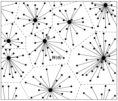
Figure 7: The dashed lines represent the boundaries of the cells. The solid lines link from the base stations to the users which they serve.

The base stations are assumed to form a Poisson point process of intensity $\lambda_{m}$ in the Euclidean plane. The users are assumed to form an independent Poisson point process of intensity $\lambda_{u}$ in the Euclidean plane. The association of the users to the closest BS makes the association region of a base station to be the Voronoi cell of this base station with respect to the collection of base stations. This association together with the downlinks are depicted in Figure 7.

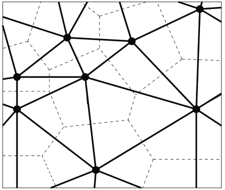
Figure 8: The solid lines represent the Delaunay graph and serve as model for the backhaul network.

The mean number of users of a typical cell, denoted by $\overline{M}$, is equal to $\lambda_{u}/\lambda_{m}$. In our model, we will assume that all users in a cell have for neighboring base stations the Delaunay neighbors of the base station which is the nucleus of the cell. This is depicted in Figure 8.

The mean number of Delaunay neighbors of a typical node is 6 and its coefficient of variation $CV(N)=\sqrt{Var(N)}/E(N)$ is $CV(N)=0.222$ (see e.g., [21]).

Hence, a rough estimate of the mean uplink radio overhead traffic is:

$$\overline{R}\approx 6\tau\frac{\lambda_{u}}{\lambda_{m}}.$$ (14)

This is only an estimate because there is a correlation between the number of users in a cell and the number of neighbors of the nucleus of this cell. We now give an upper bound on $\overline{R}$ in complement of this estimate.

The second moment of the number of users in a cell is (see [21]):

$$E(M^{2})=\frac{\lambda_{u}}{\lambda_{m}}+1.280\frac{\lambda_{u}^{2}}{\lambda_{m}^{2}}.$$ (15)

The second moment of the number of neighbors of a cell is given by:

$$E(N^{2})=Var(N)+E(N)^{2}=37.7742.$$ (16)

One can then use the Cauchy-Schwarz inequality to get the following upper-bound:

$$\overline{R}\leq\tau\sqrt{\left(\frac{\lambda_{u}}{\lambda_{m}}+1.280\frac{\lambda_{u}^{2}}{\lambda_{m}^{2}}\right)E(N^{2})}~{}.$$ (17)

Consider now a typical backhaul link, namely a typical Delaunay edge. A rough estimate of the mean backhaul overhead traffic on this link is then given by:

$$\overline{B}=2\overline{R}\approx 12\tau\frac{\lambda_{u}}{\lambda_{m}}.$$ (18)

The Cauchy-Schwarz inequality can again be used to get an upper-bound.

5.2.2 Macro and Small Cell Model

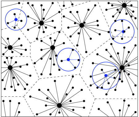
Figure 9: The discs represent the small cells. The solid lines again represent the links from the base stations to the users they serve.

In this section, we assume that each small cell has a radius of coverage and that all users covered by the small cell are attached to it. We also assume that small cell rarely overlap. The users not covered by a small cell are attached to the closest macro base station. This is depicted in Figure 9.

We assume that the small cell base stations form an independent point process of intensity $\lambda_{s}$ and that the radius of coverage is $\rho$. The mean number of users in a small cell is thus given by:

$$\overline{M}_{s}=\lambda_{u}\pi\rho^{2}$$ (19)

while the mean number of users attached to a macro cell is given by:

$$\overline{M}_{m}=\frac{\lambda_{u}}{\lambda_{m}}-\lambda_{u}\lambda_{s}\pi\rho^{2}.$$ (20)

This formula is only valid under that the Boolean model with intensity $\lambda_{s}$ and radius $\rho$ has only rare intersections of balls.

We declare neighbors of a macro cell its macro cell neighbors, defined as above, and all small cells whose base station is located in the macro cell in question or in one of its neighboring macro cells.

We declare neighbors of a small cell the base station of the macro cell it is located in and the macro neighbors of the latter as well as the small cells located in these macro cells.

Since the mean number of small cells per macro cell is $\frac{\lambda_{s}}{\lambda_{m}}$, the mean number of small cells neighbors of a macro cell is:

$$\overline{N}_{m}^{s}=7\frac{\lambda_{s}}{\lambda_{m}},$$ (21)

while the mean number of macro cells neighbor of a macro cell is still 6.

The mean number of macro cells neighbors of a small cell is 7 and the mean number of small cells neighbor of a small cell is:

$$\overline{N}_{s}^{m}=7\frac{\lambda_{s}}{\lambda_{m}}~{}.$$ (22)

Thus, the mean uplink radio overhead traffic on a macro cell is given by:

$$\overline{R}_{m} \approx 6\tau\overline{M}_{m}+\overline{N}_{m}^{s}\overline{M}_{s}$$ (23)

$$\approx 6\tau\left(\frac{\lambda_{u}}{\lambda_{m}}-\lambda_{u}\lambda_{s}\pi\rho^{2}\right)+7\tau\frac{\lambda_{s}}{\lambda_{m}}\left(\lambda_{u}\pi\rho^{2}\right)$$

whereas that on a small cell is given by:

$$\overline{R}_{s} \approx 7\tau\overline{M}_{m}+\overline{N}_{s}^{m}\overline{M}_{s}$$ (24)

$$\approx 7\tau\left(\frac{\lambda_{u}}{\lambda_{m}}-\lambda_{u}\lambda_{s}\pi\rho^{2}\right)+7\tau\frac{\lambda_{s}}{\lambda_{m}}\left(\lambda_{u}\pi\rho^{2}\right).$$

The mean backhaul traffic on a link between two macro base stations is $2\overline{R}_{m}$, whereas that between a macro base station and a small base station is equal to $\overline{R}_{m}+\overline{R}_{s}$.

These mean values can be complemented by bounds using second moments.

6 Conclusion

In this paper, we analyzed the problem of radio resource allocation in heterogeneous cellular networks composed of macro and small cells with unpredictable cell and user patterns. To solve the problem, we proposed a joint optimization of channel selection, user association and power control. The proposed solution, which is based on the Gibbs sampler, is implementable in a distributed manner and nevertheless achieves minimal system-wide potential delay, regardless of the initial state. We investigated its performance and estimated the expected overhead. Simulation result and comparison to today’s default operations have shown its high effectiveness in terms of energy consumption. Because of its operational simplicity, this distributed optimization approach is expected to play an important role in the future of heterogeneous wireless networks.

Table:

Table 1: User average throughput: b/s/Hz,  Power efficiency: b/s/Hz/W

	Default Operation	After Optimization	Performance Gain (times)
$M$ = 32, $K$ = 1	0.245, 0.0143	1.216, 1.937	4.96, 135
$M$ = 64, $K$ = 2	0.312, 0.0186	1.583, 2.685	5.07, 144
$M$ = 96, $K$ = 3	0.356, 0.0210	1.829, 3.149	5.14, 150
$M$ = 160, $K$ = 5	0.368, 0.0228	1.973, 3.488	5.36, 153

Figures:

References

- [1] Schmelz LC, van den Berg JL, Litjens R, Zetterberg K, Amirijoo M, Spaey K, Balan I, Scully N, Stefanski S: Self-organisation in wireless networks - use cases and their interrelations. In Wireless World Res. Forum Meeting 22 2009:1–5.
- [2] Sesia S, Toufik I, Baker M: LTE - The UMTS Long Term Evolution: From Theory to Practice. John Wiley & Son, 2 edition 2011.
- [3] Chen CS, Baccelli F: Self-optimization in mobile cellular networks: power control and user association. In IEEE International Conference on Communications 2010:1–6.
- [4] Hasan Z, Boostanimehr H, Bhargava V: Green cellular networks: a survey, some research issues and challenges. IEEE Communications Surveys & Tutorials 2011, 13(4):524–540.
- [5] Saunders S, Carlaw S, Giustina A, Bhat RR, Rao VS, Siegberg R: Femtocells: Opportunities and Challenges for Business and Technology. John Wiley & Sons, New York 2009.
- [6] 3GPP TS 36942: Evolved universal terrestrial radio access (EUTRA): radio frequency system scenarios. Tech. spec. v10.2.0 2011.
- [7] Luo ZQ, Zhang S: Dynamic spectrum management: complexity and duality. IEEE J. Sel. Topics in Signal Processing 2008, 2:57–73.
- [8] Chen CS, Shum KW, Sung CW: Round-robin power control for the weighted sum rate maximisation of wireless networks over multiple interfering links. European Transactions on Telecommunications 2011, 22(8):458–470.
- [9] Ahmed N, Keshav S: SMARTA: a self-managing architecture for thin access points. In ACM CoNEXT 2006:1–12.
- [10] Broustis I, Papagiannaki K, Krishnamurthy SV, Faloutsos M, Mhatre V: MDG: measurement-driven guidelines for 802.11 WLAN design. In ACM MobiCom 2007:254–265.
- [11] Chiang M, Tan CW, Palomar DP, O’Neill D, Julian D: Power control by geometric programming. IEEE Trans. Wireless Commun. 2007, 6(7):2640–2651.
- [12] Chen CS, Øien GE: Optimal power allocation for two-cell sum rate maximization under minimum rate constraints. In IEEE International Symposium on Wireless Communication Systems 2008:396–400.
- [13] Qian L, Zhang YJ, Huang J: MAPEL: achieving global optimality for a non-convex wireless power control problem. IEEE Trans. Wireless Commun. 2009, 8(3):1553–1563.
- [14] Geman S, Geman D: Stochastic relaxation, Gibbs distributions, and the Bayesian restoration of images. IEEE Transactions on Pattern Analysis and Machine Intelligence 1984, PAMI-6(6):721–741.
- [15] Brémaud P: Markov Chains: Gibbs Fields, Monte Carlo Simulation, and Queues. Springer Verlag 1999.
- [16] Massoulié L, Roberts J: Bandwidth sharing: objectives and algorithms. IEEE/ACM Trans. Netw. 2002, 10(3):320–328.
- [17] Coucheney P, Gaujal B, Touati C: Self-optimizing routing in MANETs with multi-class flows. In IEEE PIMRC 2010:2751–2756.
- [18] Liu JS, Wong WH, Kong A: Covariance structure and convergence rate of the Gibbs sampler with various scans. Journal of the Royal Statistical Society. Series B. (Methodological) 1995, 57:157–169.
- [19] 3GPP TS 36331: Evolved universal terrestrial radio access (EUTRA) radio resource control (RRC): protocol specification. Tech. spec. v10.4.0 2011.
- [20] IEEE 80220 Working Group on Mobile Broadband Wireless Access: Channel models document. 3GPP–3GPP2 Tech. Rep. 2007.
- [21] Møller J: Lectures on Random Voronoi Tessellations. Springer-Verlag, New York 1994.
- [22] Chen CS, Baccelli F, Roullet L: Joint optimization of radio resources in small and macro cell networks. In IEEE 73rd Vehicular Technology Conference (VTC Spring) 2011:1–5.
Table: