Comparison of cosmological parameter inference methods applied to supernovae lightcurves fitted with SALT-II

Abstract

We present a comparison of two methods for cosmological parameter inference from supernovae Ia lightcurves fitted with the SALT-II technique. The standard chi-square methodology and the recently proposed Bayesian hierarchical method (BHM) are each applied to identical sets of simulations based on the 3-year data release from the Supernova Legacy Survey (SNLS3), and also data from the Sloan Digital Sky Survey (SDSS), the Low Redshift sample and the Hubble Space Telescope (HST), assuming a concordance $\Lambda$CDM cosmology. For both methods, we find that the recovered values of the cosmological parameters, and the global nuisance parameters controlling the stretch and colour corrections to the supernovae lightcurves, suffer from small biasses. The magnitude of the biasses is similar in both cases, with the BHM yielding slightly more accurate results, in particular for cosmological parameters when applied to just the SNLS3 single survey data sets. Most notably, in this case, the biasses in the recovered matter density $\Omega_{\rm m,0}$ are in opposite directions for the two methods. For any given realisation of the SNLS3-type data, this can result in a $\sim 2\sigma$ discrepancy in the estimated value of $\Omega_{\rm m,0}$ between the two methods, which we find to be the case for real SNLS3 data. As more higher and lower redshift SNIa samples are included, however, the cosmological parameter estimates of the two methods converge.

1 Introduction

It has long been recognised that astronomical standard candles are of great value in constraining cosmological models. The basic argument is very straightforward. The luminosity distance $D_{\rm L}$ to an object of absolute luminosity $L$, from which one measures the flux $F$, is given by

$$D_{\rm L}\equiv\left(\frac{L}{4\pi F}\right)^{1/2}.$$ (1)

Thus the distance modulus $\mu=m-M$ between the apparent magnitude $m\equiv-2.5\log_{10}F$ of the object and its absolute magnitude $M$ is given by

$$\mu=5\log_{10}\left(\frac{D_{\rm L}}{\mbox{Mpc}}\right)+25,$$ (2)

where the constant offset ensures the usual convention that $\mu=0$ at $D_{\rm L}=10$ pc.

In a standard FRW cosmological model containing cold dark matter and dark energy, defined by the usual cosmological parameters ${\mathscr{C}}=\{\Omega_{\rm m,0},\Omega_{\rm de,0},H_{0},w\}$, the luminosity distance to an object of redshift $z$ is given by

$$D_{\rm L}(z,{\mathscr{C}})=\frac{c}{H_{0}}\frac{(1+z)}{\sqrt{|\Omega_{k,0}|}}S(\sqrt{|\Omega_{k,0}|}I(z)),$$ (3)

where

$$I(z)\!\ \equiv\!\!\int_{0}^{z}\!\!\!\frac{d\bar{z}}{\sqrt{(1+\bar{z})^{3}\Omega_{\rm m,0}\!+\!(1+\bar{z})^{3(1+w)}\Omega_{\rm de,0}\!+\!(1+\bar{z})^{2}\Omega_{k,0}}},$$ (4)

in which (neglecting the present-day energy density in radiation) $\Omega_{k,0}\equiv 1-\Omega_{{\rm m},0}-\Omega_{\rm de,0}$ and $S(x)=x$, $\sin x$ or $\sinh x$ for a spatially-flat ($\Omega_{k,0}=0$), closed ($\Omega_{k,0}<0$) or open ($\Omega_{k,0}>0$) universe, respectively. The special case $w=-1$ corresponds to a cosmological constant, for which one usually denotes the present-day density parameter by $\Omega_{\Lambda,0}$.

Thus, by measuring the distance moduli and redshifts of a set of objects ($i=1,2,\ldots,N$) of known absolute magnitude (standard candles), and considering the difference

$$\Delta\mu_{i}=\mu_{i}^{\rm obs}-\mu(z_{i},{\mathscr{C}})$$ (5)

between the observed and predicted distance modulus for each object (often termed Hubble diagram residuals), one can place constraints on the cosmological parameters ${\mathscr{C}}$. One should note, however, that in the case where the standard candles share a common, but unknown, absolute magnitude $M$, this value is exactly degenerate with the Hubble constant $H_{0}$, as is clear from (1) and (3).

In practice, there are no perfect astronomical standard candles. Type-Ia supernovae (SNIa), for example, have absolute magnitudes that vary by about $\pm 0.8$ mag in the $B$-band due to physical differences in how each supernova is triggered and also due to absorption by its host galaxy. Nonetheless, SNIa do constitute a set of ‘standardizable’ candles, since by applying small corrections to their absolute magnitudes, derived by fitting multi-wavelengths observations of their lightcurves, one can reduce the scatter considerably, to around $\pm 0.15$ mag in the $B$-band. In essence, SNIa with broader lightcurves and slower decline rates are intrinsically brighter than those with narrower lightcurves and fast decline rates (Phillips 1993; Hamuy et al. 1996).

SNIa lightcurve fitting techniques fall into two categories: those that give a direct estimate of the distance modulus, such as the Multi Colour Light Curve Shape (MLCS) method (Jha et al., 2007) and those that give estimates of the supernova apparent magnitude, lightcurve shape and colour, which can be translated into distance modulus via supernovae global parameters that must be inferred simultaneously with the cosmological parameters. This latter category of techniques includes lightcurve fitting methods, such as the Spectral Adaptive Lightcurve Template method, (SALT) (Guy et al., 2005; Astier et al., 2006), SALT-II (Guy et al., 2010) and SiFTO (Conley et al., 2008). It is this latter category of methods with which this paper is concerned, and in particular the SALT-II methodology. Another important difference between the two categories of lightcurve fitter is that the former infers the SNIa distance moduli directly, which are then used to infer the cosmological parameters, whereas the latter divides the process into two steps: first the lightcurves are fitted to obtain SNIa light curve parameters such as $\hat{m}^{*}_{B,i},\hat{c}_{i},\hat{x}_{1,i}$ which are then used to infer cosmological parameters simultaneously with the SNIa global parameters $\alpha,\beta,M_{0}$, in a second step. This therefore provides an opportunity to use the products of the first step of the SALT-II analysis, namely the stretch, colour and absolute B-band magnitude $(\hat{m}^{*}_{B,i},\hat{c}_{i},\hat{x}_{1,i})$ as the inputs to alternative methods for inferring cosmological parameters.

In this paper, we take advantage of this opportunity and perform a comparison of cosmological inference methods using supernovae lightcurves fitted with SALT-II. In particular, we compare the standard $\chi^{2}$-method which is widely used in the analysis of SNIa, and the Bayesian hierarchical method (BHM), which was recently proposed by March et al. (2011). For varying implementations of the standard $\chi^{2}$-method, see for example Astier et al. (2006); Kowalski et al. (2008); Kessler et al. (2009a); Amanullah et al. (2010); Guy et al. (2010); Conley et al. (2011); Marriner et al. (2011). The comparison is performed by applying both methods to sets of realistic simulated SN data based on the real 3-year data release from the Supernova Legacy Survey (SNLS3) (Conley et al., 2011; Guy et al., 2010), together with a compilation of various other samples at lower and higher redshift suggested and supplied by the SNLS3 team. We also apply both inference methods to the real SNLS3 single survey data set to compare the cosmological parameter inferences obtained from the two approaches.

The outline of this paper is as follows. In Section 2, we give a short summary of SALT-II lightcurve fits, followed by a brief description of the standard $\chi^{2}$-method and BHM for inferring cosmological parameters from SNIa lightcurves fitted with SALT-II. In Section 3, we describe the real SNLS3 data set along with the real SDSS, HST and LowZ samples on which our simulations are based, and then discuss our simulation process in Section 4. The statistical comparison of the $\chi^{2}$-method and BHM, as applied to our simulated data sets, is described in Section 5, and the results of applying the two methods to the real data are presented in Section 6. We conclude in Section 7.

Finally, we note that this paper may be considered as complementary to our companion paper (Karpenka et al. 2012), in which we use an extension of the BHM to constrain the properties of dark matter haloes of foreground galaxies along the lines-of-sight to (a subset of) the SNIa in the SNLS3 catalogue, assuming a fixed background cosmology.

2 Cosmological inference methods

Cosmological parameter inference takes place after the selection cuts, lightcurve fitting and Malmquist correction stages of the analysis process have been implemented (see Section 3). The most widely used method for cosmological parameter inference from SALT-II fitted lightcurves is the basic minimization of the chi-square statistic, although there are a few differences in the way in which this method is implemented, as outlined below. More recently, March et al. (2011) proposed a Bayesian hierarchical method (BHM), which provides a robust statistical framework for the full propagation of systematic uncertainties to the final inferences. We give a brief outline of these two alternative approaches below, but note that in our subsequent analyses the SNIa data input to the two methods are the same, having had the same selection cuts, fits and corrections made.

For each selected SNIa, in addition to an estimate $\hat{z}$ of its redshift and an associated uncertainty $\sigma_{z}$, derived from observations of its host galaxy, we take as our basic data the output from the SALT-II lightcurve fitting method, which produces the best-fit values: $\hat{m}_{B}^{\ast}$, the rest frame $B$-band apparent magnitude of the supernovae at maximum luminosity; $\hat{x}_{1}$, the stretch parameter related to the width of the fitted light curve; and $\hat{c}$, the colour excess in the $B$-band at maximum luminosity. These are supplemented by the covariance matrix of the uncertainties in the estimated lightcurve parameters, namely

$$\widehat{C}=\left(\begin{array}[]{ccc}\sigma^{2}_{m^{\ast}_{B}}&\sigma_{m^{\ast}_{B},x_{1}}&\sigma_{m^{\ast}_{B},c}\\[5.69054pt] \sigma_{m^{\ast}_{B},x_{1}}&\sigma^{2}_{x_{1}}&\sigma_{x_{1},c}\\[5.69054pt] \sigma_{m^{\ast}_{B},c}&\sigma_{x_{1},c}&\sigma^{2}_{c}\\ \end{array}\right).$$ (6)

Therefore, our basic input data for each SN ($i=1,\ldots,N_{\rm SN}$) are

$$D_{i}\equiv\{\hat{z}_{i},\hat{m}_{B,i}^{\ast},\hat{x}_{1,i},\hat{c}_{i}\},$$ (7)

and we assume (as is implicitly the case throughout the SN literature) that the vector of values $(\hat{m}_{B,i}^{\ast},\hat{x}_{1,i},\hat{c}_{i})$ for each SN is distributed as a multivariate Gaussian about the true values, with covariance matrix $\widehat{C}_{i}$.

2.1 Standard $\chi^{2}$-method

The standard method of cosmological parameter inference used with outputs from the SALT-II lightcurve fitter is a basic chi-square minimization technique, see for example Astier et al. (2006); Kowalski et al. (2008); Kessler et al. (2009a); Amanullah et al. (2010); Guy et al. (2010); Conley et al. (2011); Marriner et al. (2011). A detailed account of this approach, together with a description of some statistical issues associated with the methodology, is given in the preceding references; we therefore present only a brief summary here.

One begins by defining the ‘observed’ distance modulus $\mu^{\rm obs}_{i}$ for the $i$th SN as

$$\mu_{i}^{\rm obs}=\hat{m}_{B,i}^{\ast}-M+\alpha\hat{x}_{1,i}-\beta\hat{c}_{i},$$ (8)

where $M$ is the (unknown) $B$-band absolute magnitude of the SN, and $\alpha$, $\beta$ are (unknown) nuisance parameters controlling the stretch and colour corrections; all three parameters are assumed to be global, i.e. the same for all SNIa.

One then defines the $\chi^{2}$ misfit function

$$\chi^{2}({\mathscr{C}},\alpha,\beta,M,\sigma_{\text{int}})=\sum_{i=1}^{N}\frac{[\mu_{i}^{\text{obs}}(\alpha,\beta,M)-\mu_{i}({\mathscr{C}})]^{2}}{\sigma_{i}^{2}(\alpha,\beta,\sigma_{\text{int}})},$$ (9)

where, for clarity, we have made explicit the functional dependencies of the various terms on (only) the parameters to be fitted. In this expression, $\mu_{i}$ is the predicted distance modulus given by (2) and is a function of SN redshift $z_{i}$ and the cosmological parameters ${\mathscr{C}}$, and the total dispersion $\sigma_{i}^{2}$ is the sum of several errors added in quadrature:

$$\sigma_{i}^{2}=\sigma_{z,i}^{2}+\sigma_{\text{int}}^{2}+\sigma_{\text{fit},i}^{2}(\alpha,\beta).$$ (10)

The three components are: (i) the error $\sigma_{z,i}$ in the redshift measurement owing to uncertainties in the peculiar velocity of the host galaxy and in the spectroscopic measurements; (ii) the intrinsic dispersion $\sigma_{\text{int}}$, which describes the global variation in the SNIa absolute magnitudes that remain after correction for stretch and colour; and (ii) the fitting error, which is given by

$$\sigma_{\text{fit},i}^{2}=\mn@boldsymbol{\psi}^{\rm t}\hat{C}_{i}\mn@boldsymbol{\psi},$$ (11)

where the transposed vector $\mn@boldsymbol{\psi}^{\rm t}=\left(1,\alpha,-\beta\right)$ and $\hat{C}_{i}$ is the covariance matrix given in (6).

Typically, the chi-squared function (9) is minimized simultaneously with respect to the cosmological parameters ${\mathscr{C}}$ and the global SNIa nuisance parameters $\alpha$, $\beta$ and $M$. There are, however, a few differences in the way in which this minimisation is performed, such as which search algorithm is used (MCMC techniques or grid searches) and the treatment of $M$ (which is degenerate with $H_{0}$), namely whether these parameters are marginalised over analytically or numerically. Once this chi-squared minimisation has been performed, the value of $\sigma_{\text{int}}$ is estimated by adjusting it to obtain $\chi^{2}/N_{\rm dof}\sim 1$, usually by some iterative process.

In this work, we take the simple_cos_fitter algorithm (Conley et al., 2011) as representative of the general class of chi-square methods, and compare its performance with the BHM, which we describe below. It should be noted that the chi-square method is an approximation to the BHM in certain limits (see Gull 1989 for a general discussion of this, and March et al. 2011 for a discussion of this as applied to the SNIa case.). Hence we expect the two methods to converge in some limit; detailed studies into this exact limit have not yet been carried out.

2.2 Bayesian hierarchical method

Recently, a more statistically well-motivated method for cosmological parameter inference from SNIa was put forward in the form of a Bayesian hierarchical model (March et al., 2011), itself based on the methodology of (Gull, 1989), and indeed is a special case of the more general methodology of (Kelly, 2007); which provides for full propagation of systematic uncertainties to the final inferences and also allows for rigorous model selection.

In essence, this method provides a means for constructing a robust effective likelihood function that yields the probability of obtaining the observed data for the $i$th SN (i.e. the parameter values obtained in the SALT-II lightcurve fits) as a function of the cosmological parameters and global SNIa nuisance parameters, namely

$$\Pr(\hat{m}_{B,i}^{\ast},\hat{x}_{1,i},\hat{c}_{i},\hat{z}_{i}|{\mathscr{C}},\alpha,\beta,\sigma_{\text{int}}),$$ (12)

which also depends on the covariance matrix $\widehat{C}_{i}$ of the uncertainties on the input data $(\hat{m}_{B,i}^{\ast},\hat{x}_{1,i},\hat{c}_{i})$, and the uncertainty $\sigma_{z,i}$ in the estimated redshift $\hat{z}_{i}$, all of which are assumed known. The full likelihood function is given by the product of the likelihoods (12) for each SN.

The likelihood for each SN is computed by first introducing the hidden variables $M_{i}$, $x_{i}$, $c_{i}$ and $z_{i}$, which are, respectively, the true (unknown) values of its absolute $B$-band magnitude, stretch and colour corrections, and redshift. These are then assigned priors, which themselves contain further nuisance parameters, and all the parameters introduced in this way are marginalised over to obtain the likelihood (12). The details of this procedure are given in Appendix A. By assuming separable Gaussian priors on the hidden variables and nuisance parameters, one can perform all the marginalisations analytically, except for two nuisance parameters $R_{x}$ and $R_{c}$, which are also described in Appendix A, that must be marginalised over numerically.

The full likelihood function is then multiplied by an assumed prior (see Appendix A) on the unknown parameters to yield their posterior distribution. This posterior is explored using the MultiNest algorithm (Feroz & Hobson, 2008; Feroz et al., 2009), which implements the nested sampling method (Skilling, 2004, 2006) adapted for potentially multimodal distributions.

3 Real supernovae data

We will perform our comparison of the standard chi-square method and the BHM by applying them to two classes of data sets. The first of these is the single survey SNLS3 data alone, i.e. only SNIa data which was taken during the first three years of the SNLS3 survey (Guy et al., 2010). We take the SNLS3 data as supplied by the SNLS3 team after selection cuts have been made, the SALT-II lightcurve fitting process has been completed and the Malmquist correction has been applied. Our interest in comparing the performance of the two cosmological parameter inference methods as applied to this single survey data set is driven by potential science applications that use a single SNIa survey in conjunction with other data sets (not SNIa) to investigate various astrophysical and cosmological phenomena. An example of such an application is constraining the properties of dark matter haloes of foreground galaxies along the lines-of-sight to the SNIa using gravitational lensing, as discussed in our companion paper (Karpenka et. al. 2012).

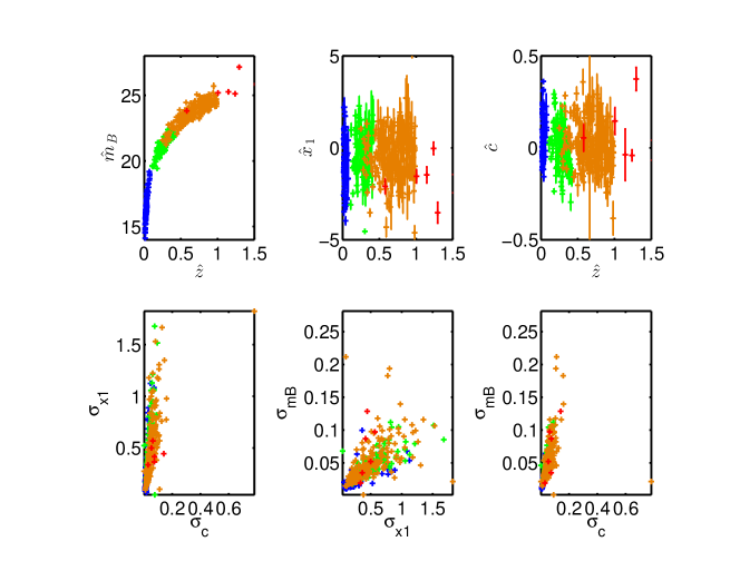
Figure 1: A simulated SNANA data set, comprising SNe from Low Z (red); SDSS (green); SNLS3 (gold) and HST (red).

For more general cosmological parameter inference applications, we are also interested in comparing the performance of the two methods on a composite ‘cosmological’ data set, since extracting good constraints on cosmological parameters from SNIa surveys requires the inclusion of both low-redshift and high-redshift samples. Since no survey currently covers both the low- and high-redshift parts of the Hubble diagram, several data sets are generally considered together to span the full redshift range. In this paper we use the compilation suggested and supplied by the SNLS3 team, which is described in Guy et al. (2010). In addition to the SNLS3 data, it is comprised of: various samples with $z<0.1$; the SDSS survey (Kessler et al., 2009a; Holtzman et al., 2008) for $0.1<z<0.4$; and high-redshift HST data (Riess & Strolger, 2007). Selection cuts, SALT-II lightcurve fitting and Malmquist corrections are made by the SNLS3 team and are already implemented in the supplied data files, as discussed in detail in Perrett et al. (2010) .

4 Simulated supernovae data

SNIa photometric data were simulated and fitted using the publicly available SNANA package (Kessler et al., 2009b). First, data were simulated to match closely the SNLS3 data set (Guy et al., 2010) by using the SNLS3 co-added simulation library files (which are publicly available as part of the SNANA package), a coherent magnitude smearing of $0.12$, and colour smearing. The colour smearing effect, or broad-band colour dispersion model, implemented in the data simulation is the EXPPOL model described by Fig. 8 of (Guy et al., 2010), and the simulated Malmquist bias is based on Fig. 14 of Perrett et al. (2010). In total 100 similar data sets of SNLS3 style SNIa were simulated.

The SNANA SNIa data simulation is a two-stage process that mimics the real data collection and analysis process. The first stage is the simulation of photometric data in accordance with the characteristic instrument and survey properties of the SNSL3 survey using the SNLS3 simulation library files mentioned above. The second stage is the lightcurve fitting process in which the photometric data are fitted to SALT-II templates to give estimates of the SNIa absolute B-band magnitude $\hat{m}_{B}$, lightcurve stretch $\hat{x}_{1}$ and colour $\hat{c}$. At this lightcurve fitting stage, basic cuts are made to discard SNIa with a low signal-to-noise ratio and/or too few observed epochs in sufficient bands. After the lightcurve fitting stage we make a redshift dependent magnitude correction for the Malmquist bias; the correction is taken from a spline interpolation of table 4 in Perrett et al. (2010). All selection cuts and Malmquist corrections take place prior to the cosmology inference step.

In addition to simulating the SNLS3 single survey data sets, we also simulate combined ‘cosmological’ data sets made by simulating individual LowZ, SDSS and HST samples which are generated separately using SNANA and the appropriate simulation templates. The LowZ sample SNIa were simulated based on the CFA3-KepplerCam lightcurves (Hicken et al., 2009) ; SDSS sample uses the SDSS 2005 templates (Holtzman et al., 2008; Kessler et al., 2009a; Lampeitl et al., 2009) and the HST sample is based on the Strolger & Riess (2006) templates. An example combined simulated data set is shown in Fig. 1.

5 Results from simulated data

In section 5.1 we analyse both the single survey SNLS3 data sets, and the combined multi survey ‘cosmology’ data sets within the framework of the $\Lambda$CDM model in which non-zero curvature is allowed. In section 5.2, we further analyse the compiled ‘cosmology’ data sets within the framework of the flat $w$CDM model in which curvature is fixed at zero, but the dark energy equation of state, $w$ is permitted to vary.

5.1 $\Lambda$CDM analysis of SNLS3 and ‘cosmological’ samples

In the $\Lambda$CDM analysis of simulated SNLS3 data alone, we find that both methods perform well, considering the difficulties that arise when attempting to obtain cosmological constraints from a survey that does not include a low-$z$ sample to anchor the lower end of the Hubble diagram.

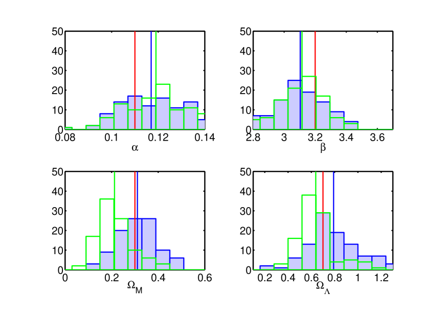
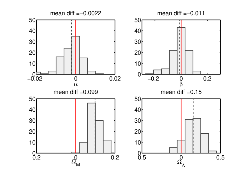
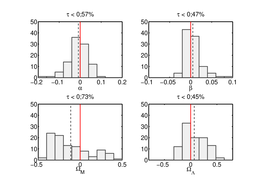
Figure 2: $\Lambda$CDM analysis of simulated SNLS3 data sets. Top 4 panels: sampling distributions derived from 100 sets of simulated data for the SNIa global parameters $\alpha,\beta$ and the cosmological parameters $\Omega_{\rm m,0},\Omega_{\Lambda,0}$, inferred using the BHM (blue histograms) and the chi-square method as implemented by the ‘simple_cos_fitter’ code (green histogram). Blue and green vertical lines show the mean value of the estimator, solid red vertical lines show the value of the true (i.e. model input) parameter. Middle 4 panels: histograms showing the raw difference in estimators between the BHM method and ‘simple_cos_fitter’ method, given by $\hat{\theta}_{\text{BHM}}-\hat{\theta}_{\chi^{2}}$. Bottom 4 panels: the difference in accuracy between the two methods, given by $\tau=\theta^{-1}_{\text{true}}(|\hat{\theta}_{\text{BHM}}-\theta_{\text{true}}|-|\hat{\theta}_{\chi^{2}}-\theta_{\text{true}}|)$. Negative values of $\tau$ indicate that the BHM estimator is closer to the true value than the simple_cos_fitter (i.e.$\chi^{2}$) estimator.

Fig. 2 (top 4 panels) shows the sampling distributions of the estimators for the parameters of interest for the BHM (blue histograms) and the $\chi^{2}$-method (green histograms), as implemented by the ‘simple_cos_fitter’. We see that both methods recover similar global SNIa parameters $\alpha,\beta$. More importantly, both methods recover the cosmological parameters $\Omega_{\rm m,0}$ and $\Omega_{\Lambda,0}$, but with small biasses that differ between the methods.

	$\Lambda$CDM
	SNLS3 only		Combined sample
Parameter	BHM	$\chi^{2}$-method	BHM	$\chi^{2}$-method
$\alpha$	$0.007$	$0.009$	$0.010$	$0.0021$
$\beta$	$-0.096$	$-0.085$	$-0.029$	$-0.075$
$\Omega_{\rm m,0}$	$0.011$	$-0.088$	$-0.037$	$-0.041$
$\Omega_{\Lambda,0}$	$0.091$	$-0.062$	$0.021$	$0.0086$

Table 1: Bias on the estimators of the parameters of interest obtained from the two cosmological inference methods, for $\Lambda$CDMmodel, as a result of the analysis of 100 sets of SNSL3 only data, and 100 sets of ‘cosmology’ data sets.

The biasses on the recovered parameter values for both methods are listed in Table 1. Perhaps most notable, is that the recovered value of $\Omega_{\rm m,0}$ in BHM is biassed slightly high, whereas that for the $\chi^{2}$ method is biassed somewhat low. Thus, when the two methods are used to analyse the same data set, they can give discrepant values for $\Omega_{\rm m,0}$. Fig. 2 (middle 4 panels) shows that the average discrepancy in $\Omega_{\rm m,0}$ for the single survey SNLS3 data is $\sim 0.1$ and the maximum discrepancy can be up to $\sim 0.2$. From the bottom 4 panels of Fig. 2 we see that in $\sim 73\%$ of trials the BHM provides an estimator for $\Omega_{\rm m,0}$ which is closer to the true value of $\Omega_{\rm m,0}$ than the estimator given by the $\chi^{2}$ method.

Analysis of the SNLS3 survey alone is useful for particular applications such as when used in conjunction with other non SNIa data sets as mentioned earlier. However, when the primary aim of the analysis is cosmological parameter inference, then several different surveys are analysed together to span an appreciable redshift range and form a ‘cosmological’ sample. In order to obtain constraints on the cosmological parameters, we analysed combined ‘cosmological’ samples described in section 4 which span a broader redshift range.

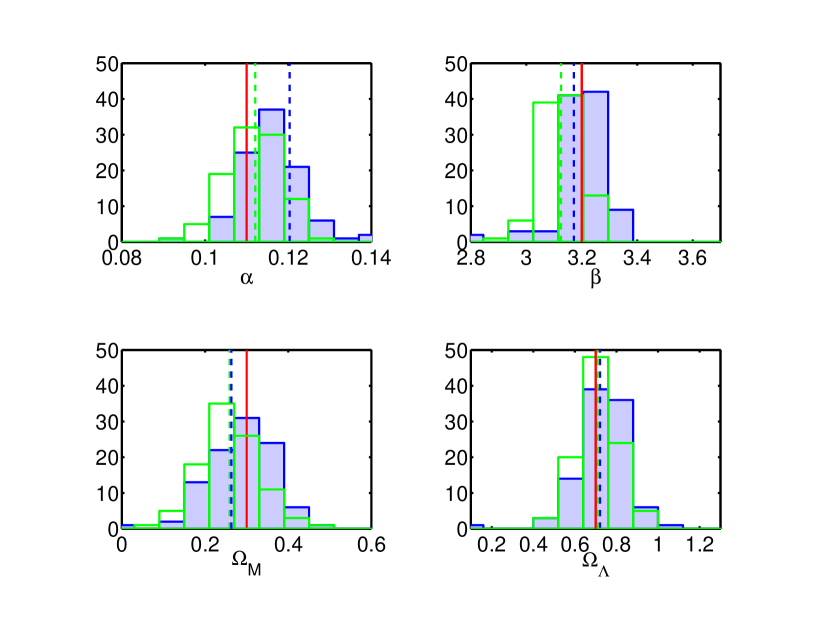
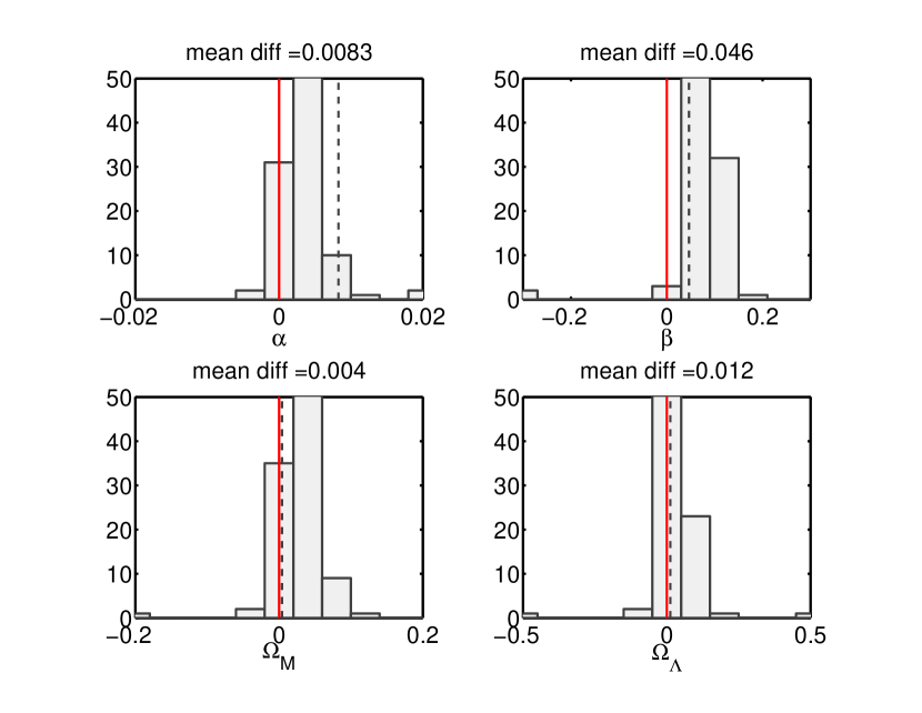
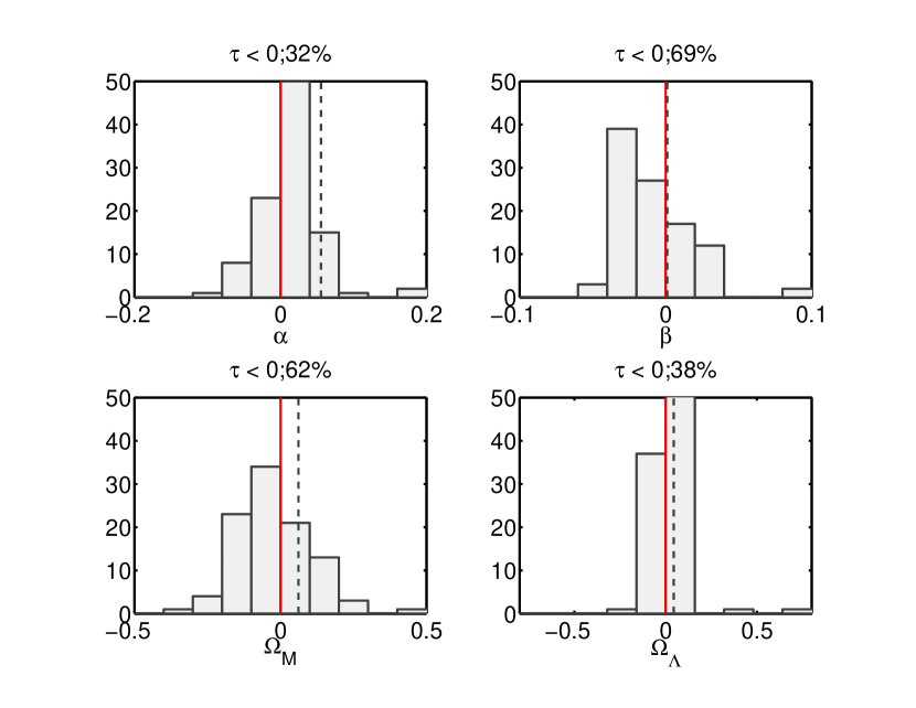
Figure 3: As for Fig. 2, but for the $\Lambda$CDM analysis of 100 simulations of the combined ‘cosmology’ data set.

The results of these analyses are presented in Fig.3. The top 4 panels show the cosmological parameter inference results when the SNLS3 SNIa are analysed jointly with the LowZ, SDSS and HST simulated samples. As can be seen by comparing the corresponding panels in Fig. 2, the width of the sampling distribution decreases when the additional low and high redshift SNIa are included in the analysis.

Increasing the redshift range of the SNIa sample also decreases the discrepancy between the estimators for the cosmological parameters given by the two inference methods. From the middle 4 panels of Fig. 2, the mean differences between the estimators for $\Omega_{\rm m,0}$ and $\Omega_{\rm\Lambda,0}$ are $0.099$ and $0.15$ respectively for the SNLS3 sample alone; whereas for the ‘cosmology’ sample the mean differences between the estimators for $\Omega_{\rm m,0}$ and $\Omega_{\rm\Lambda,0}$ decrease to $0.004$ and $0.012$ respectively, as can be seen in the middle 4 panels of Fig.3.

5.2 $w$CDM analysis of combined ‘cosmological’ sample

As well as the standard $\Lambda$CDM model of the Universe, many theories of dark energy have been put forward which have a dark energy equation of state such that $w\neq-1$ (for some examples of comprehensive reviews see Amendola & Tsujikawa 2010; Frieman et al. 2008; Peebles & Ratra 2003). The dark energy equation of state, $w$ is highly degenerate with curvature, a degeneracy which cannot be broken with a geometric probe alone such as the SNIa. Hence we perform the cosmological parameter inference within the $w$CDM model in the context of a flat Universe for which $\Omega_{k,0}\equiv 0$.

The SNLS3 sample alone do not cover a broad enough redshift range to give meaningful constraints on $w$, hence we only present a cosmological parameter inference for the $w$CDM model using the combined ‘cosmology’ samples. The results of the $w$CDM analysis for the simulated ‘cosmological’ SNIa data sets for the BHM and $\chi^{2}$ methods are presented in Fig.4 and Table 2.

	$w$CDM
	Combined sample
Parameter	BHM	$\chi^{2}$-method
$\alpha$	$0.0050$	$0.0021$
$\beta$	$0.0063$	$-0.0076$
$\Omega_{\rm m,0}$	$-0.023$	$-0.043$
$w$	$-0.050$	$-0.034$

Table 2: Bias on the estimators of the parameters of interest for the $w$CDM model, obtained from the two cosmological inference methods applied to the 100 simulated sets of ‘cosmological’ samples.

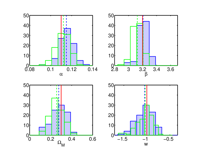
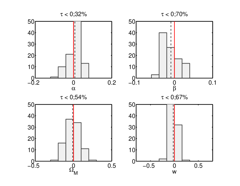
Figure 4: As for Fig. 2, but for the $w$CDM analysis of 100 simulations of the combined ‘cosmology’ data set.

6 Results from real data

We applied both parameter inference methods to the real SNLS3 single survey data set, and the combined ‘cosmological’ data set described in section 3, for the $\Lambda$CDM model and $w$CDM model. The data sets supplied by the SNLS team are a linearly transformed version of the SALT-II parameters (Guy et al., 2010), hence it is not meaningful to compare the transformed SNIa global parameters $\alpha,\beta$ with the corresponding parameters in our standard SALT-II.

Figure 5: Contour plots for $\Lambda$CDM analysis of real and simulated SNLS3 data sets. Contours enclose $68.3\%$ and $95.4\%$ of the posterior mass or likelihood for the BHM (blue) and $\chi^{2}$ (green) methods. Blue and green stars show the locations of the estimators for the BHM and $\chi^{2}$ methods respectively. The upper plot shows the analysis of the real data, and the lower plot the simulated data. For the analysis of the simulated data, a red star indicates the location of the true model input parameters.

6.1 $\Lambda$CDM analysis of SNLS3 sample

We present the cosmological parameter inference for the $\Lambda$CDM model using only SNLS3 data in Fig. 5. The upper plot in shows the $68.3\%$ and $95.4\%$ contours for the real SNLS3 only data set. Contours from the BHM are shown in blue, and contours from the $\chi^{2}$ method in green. The estimators for the parameters for both methods are the expectation values of the 1-D marginalised posteriors (BHM) or likelihoods ($\chi^{2}$), the estimators for the BHM are indicated with a blue star, and the estimators for the $\chi^{2}$ with a green star. Of note is the discrepancy of $~{}2\sigma$ in the inference of $\Omega_{\rm m,0}$ and $\Omega_{\rm\Lambda,0}$, corresponding to a difference of $~{}0.2$ units of $\Omega_{\rm m,0}$. A discrepancy of this magnitude does fall within the expected range of mean differences (see Fig.2) although it does lie towards the tail of the mean-difference distribution. The lower panel of Fig. 5 shows an example analysis of a corresponding simulated SNLS3 only data set. Additionally, this lower plot includes a red star to indicate the location of the model input parameters from which the simulated data set was generated.

6.2 $\Lambda$CDM analysis of combined ‘cosmological’ sample

Including the additional high and low redshift SNIa that make up the ‘cosmological’ sample significantly reduces the discrepancy between estimators for $\Omega_{\rm m,0}$ and $\Omega_{\rm\Lambda,0}$ obtained using the two different inference methods, as shown in Fig. 6. As expected, for the real data, increasing the redshift range of the data set greatly enhances the ability of the SNIa to constrain $\Omega_{\rm m,0}$ and $\Omega_{\rm\Lambda,0}$.

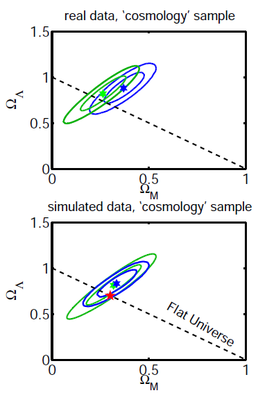
Figure 6: As for Fig. 6, but for $\Lambda$CDM analysis of real and simulated combined ‘cosmological’ data sets.

Similarly, for the simulated data, including the additional high and low redshift SNIa decreases the discrepancy between the estimators for the two methods, and increases the constraining power of the SNIa. Interestingly, for this particular realization of the simulated data, both methods give almost the same values for $\Omega_{\rm m,0}$ and $\Omega_{\rm\Lambda,0}$, which are yet $~{}1\sigma$ distant from the true values. There is scope for further investigation as to when the two methods converge, under what circumstances each method is more accurate, and in what limit the BHM reduces to the $\chi^{2}$ approximation for parameter inference.

6.3 $w$CDM analysis of combined ‘cosmological’ sample

In Fig. 7 we present the analysis of the real ‘cosmology’ data set for the flat $w$CDM model (upper plot), and compare it with a corresponding simulated data set (lower panel). The same simulated data set is used in the lower panels of both Fig. 6 and 7. The discrepancy of $~{}0.2$ units of $w$ between the inferred values for the dark energy equation of state recovered for the real data set by the two inference methods is just within the expected range for the mean difference, as shown in Fig.4. As previously, this particular realisation of simulated data gives a very small discrepancy between the value of the estimators for the two methods.

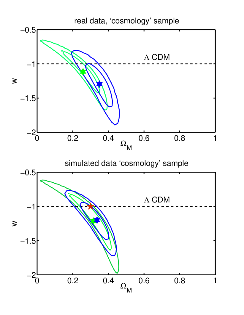
Figure 7: As for Fig. 6, but for $w$CDM analysis of real and simulated combined ‘cosmological’ data sets.

7 Conclusions

Through the analysis of realistic simulated SNe data sets, we have established that the BHM and $\chi^{2}$ cosmological parameter inference methods give different but comparable results when applied to the same data. Both methods suffer from small biasses in the recovery of cosmological parameters and the discrepancy between the two methods is greatest when only a single survey such as SNLS3 is used. In this case, we find that the BHM gives slightly less biassed results, particularly on the value of $\Omega_{\rm m,0}$. Moreover, the biasses on $\Omega_{\rm m,0}$ are in opposite directions for the two methods, which an result in a $\sim 2\sigma$ discrepancy in its estimated value for any given realisation of the SNLS3-type data. Indeed, we find this to be the case for the real SNLS3 data set. The discrepancy between the methods diminishes, however, as the redshift range of the data set increases. As more higher and lower redshift SNIa are added to the sample, the two methods begin to converge on their estimate for the cosmological parameters of interest.

We note that we have investigated the difference between the parameter inferences obtained for two methods for a given pre-selected, pre-corrected data set. One cannot over-emphasise, however, the importance of the preceding selection cuts and Malmquist bias corrections for obtaining accurate estimates of the underlying cosmological parameters. Current SNIa data sets have been spectroscopically selected, which ensures a high degree of purity of sample, but future large SN scale surveys such as the Dark Energy Survey will rely heavily on photometric classification (Bernstein et al., 2012). For a discussion of how photometric selection methods affect the cosmological parameter inference independently of how the parameter inference step is performed, see Sako et al. (2011).

Finally, we also point out that our investigation has been carried out specifically in the context of the SALT-II fitted SNIa data. We believe this analysis to be of use to the community, as the SALT-II light curve fitter is one of the most widely used (along with MLCS) and many current surveys have released their SNIa data in this SALT-II fitted format. We look forward to the future as increasingly sophisticated light curve fitting techniques (e.g.Mandel et al. (2009)) and cosmological parameter inference methods (e.g. Shafieloo et al. (2012); Seikel et al. (2012)) gradually supersede current methods, but in the meantime we offer this study into the comparative performance of two different cosmological parameter inference techniques that are currently used in conjunction with the SALT-II light curve fitter.

8 Acknowledgements

We thank Rick Kessler and John Marriner for extensive advice and assistance in simulating data with SNANA. We thank Heather Campbell for advice on the SDSS Malmquist bias. We are grateful for useful conversations and comments from Mark Sullivan, Julien Guy, Mat Smith, Roberto Trotta. NVK acknowledges support from the Swedish Research Council (contract No. 621-2010-3301). FF is supported by a Research Fellowship from Trinity Hall, Cambridge.

Appendix A Form of the BHM likelihood function

For each SN, we seek the likelihood (12) of the input data given the parameters of our model, namely

$$\Pr(\hat{m}_{B,i}^{\ast},\hat{x}_{1,i},\hat{c}_{i},\hat{z}_{i}|{\mathscr{C}},\alpha,\beta,\sigma_{\text{int}},\widehat{C}_{i},\sigma_{z,i}),$$ (13)

where, for completeness, we have included the dependence on the assumed known uncertaintes $\widehat{C}_{i}$ and $\sigma_{z,i}$. As discussed in Section 2.2, we compute this likelihood by first introducing the hidden variables $M_{i}$, $x_{1,i}$, $c_{i}$ and $z_{i}$, which are, respectively, the true (unknown) values of its absolute $B$-band magnitude, stretch and colour corrections, and redshift; these are then assigned priors and marginalised over to obtain the likelihood (13).

For the sake of brevity, we denote the (global) model parameters in (13) that we wish to constrain by $\mn@boldsymbol{\phi}=\{{\mathscr{C}},\alpha,\beta,\sigma_{\text{int}}\}$ and those assumed known (and different for each SN) by $\mn@boldsymbol{\psi}_{i}=\{\widehat{C}_{i},\sigma_{z,i}\}$. Thus, introducing the hidden variables $M_{i}$, $x_{1,i}$, $c_{i}$ and $z_{i}$, the likelihood (13) can be written as

$$\Pr(\hat{m}_{B,i}^{\ast},\hat{x}_{1,i},\hat{c}_{i},\hat{z}_{i}|\mn@boldsymbol{\phi},\mn@boldsymbol{\psi})=\int dM_{i}\,dx_{1,i}\,dc_{i}\,dz_{i}\,\Pr(\hat{m}_{B,i}^{\ast},\hat{x}_{1,i},\hat{c}_{i},\hat{z}_{i}|\mn@boldsymbol{\phi},\mn@boldsymbol{\psi},M_{i},x_{1,i},c_{i},z_{i})\Pr(M_{i},x_{i},c_{i},z_{i}|\sigma_{\text{int}}).$$ (14)

Assuming that the measured redshift $\hat{z}_{i}$ is independent of $\hat{m}_{B,i}^{\ast}$, $\hat{x}_{1,i}$ and $\hat{c}_{i}$, and, similarly, that the true redshift $z_{i}$ is independent of $M_{i}$, $x_{i}$, $c_{i}$, one may write

$$\Pr(\hat{m}_{B,i}^{\ast},\hat{x}_{1,i},\hat{c}_{i},\hat{z}_{i}|\mn@boldsymbol{\phi},\mn@boldsymbol{\psi})=\int dz_{i}\,\Pr(\hat{z}_{i}|z_{i},\sigma_{z,i})\Pr(z_{i})\,\int dM_{i}\,dx_{1,i}\,dc_{i}\,\Pr(\hat{m}_{B,i}^{\ast},\hat{x}_{1,i},\hat{c}_{i}|\mn@boldsymbol{\phi},\mn@boldsymbol{\psi},M_{i},x_{1,i},c_{i},z_{i})\Pr(M_{i},x_{1,i},c_{i}|\sigma_{\text{int}}).$$ (15)

where $\Pr(z_{i})$ is the prior on the true SN redshift, and the prior $\Pr(M_{i},x_{1,i},c_{i}|\sigma_{\text{int}})$ can itself be expanded as

$$\Pr(M_{i},x_{1,i},c_{i}|\sigma_{\text{int}})=\int dM_{0}\,dx_{\ast}\,dR_{x}\,dc_{\ast}\,dR_{c}\,\Pr(M_{i},x_{1,i},c_{i}|M_{0},\sigma_{\text{int}},x_{\ast},R_{x},c_{\ast},R_{c})\Pr(M_{0},x_{\ast},R_{x},c_{\ast},R_{c}|\sigma_{\text{int}}),$$ (16)

in which we have introduced the nuisance hyperparameters $M_{0}$, $x_{\ast}$, $R_{x}$, $c_{\ast}$ and $R_{c}$ associated with the SN population and described below. Equations (15) and (16) form the basis for the Bayesian hierarchical model of March et al. (2011).

To proceed further, one first assumes that both of the joint prior distributions in the integrand of (16) are separable, as follows:

$$\Pr(M_{i},x_{1,i},c_{i}|M_{0},\sigma_{\text{int}},x_{\ast},R_{\ast},c_{\ast},R_{\ast}) = \Pr(M_{i}|M_{0},\sigma_{\text{int}})\Pr(x_{1,i}|x_{\ast},R_{x})\Pr(c_{i}|c_{\ast},R_{c}),$$ (17)

$$\Pr(M_{0},x_{\ast},R_{\ast},c_{\ast},R_{\ast}|\sigma_{\text{int}}) = \Pr(M_{0})\Pr(x_{\ast})\Pr(R_{x})\Pr(c_{\ast})\Pr(R_{c}).$$ (18)

One then assigns a form for the prior distribution of each of the hidden parameters $M_{i}$, $x_{1,i}$, $c_{i}$, $z_{i}$ and nuisance hyperparameters $M_{0}$, $x_{\ast}$, $R_{x}$, $c_{\ast}$, $R_{c}$. These are taken to be: $\Pr(M_{i}|M_{0},\sigma_{\text{int}})={\cal N}(M_{0},\sigma_{\rm int}^{2})$, $\Pr(x_{1,i}|x_{\ast},R_{x})={\cal N}(x_{\ast},R_{x}^{2})$, $\Pr(c_{i}|c_{\ast},R_{c})={\cal N}(c_{\ast},R_{c}^{2})$, $\Pr(z_{i})=1$, $\Pr(M_{0})={\cal N}(\bar{M}_{0},\sigma_{M_{0}}^{2})$, $\Pr(x_{\ast})={\cal N}(0,\sigma_{x_{\ast}}^{2})$, $\Pr(c_{\ast})={\cal N}(0,\sigma_{c_{\ast}}^{2})$, $\Pr(R_{x})=1/R_{x}$ and $\Pr(R_{c})=1/R_{c}$, where one assumes $\bar{M}_{0}=-19.3$ mag, $\sigma_{M_{0}}=2.0$ mag, $\sigma_{x_{\ast}}=1$ and $\sigma_{c_{\ast}}=1$.

The only remaining probability distributions required to evaluate (15) are $\Pr(\hat{z}_{i}|z_{i},\sigma_{z,i})$ and $\Pr(\hat{m}_{B,i}^{\ast},\hat{x}_{1,i},\hat{c}_{i}|\mn@boldsymbol{\phi},\mn@boldsymbol{\psi},M_{i},x_{1,i},c_{i},z_{i})$. The former is given simply by $\Pr(\hat{z}_{i}|z_{i},\sigma_{z,i})={\cal N}(z_{i},\sigma_{z,i}^{2})$ and the latter is the multivariate Gaussian

$$\Pr(\hat{m}_{B,i}^{\ast},\hat{x}_{1,i},\hat{c}_{i}|\mn@boldsymbol{\phi},\mn@boldsymbol{\psi},M_{i},x_{1,i},c_{i},z_{i})=|2\pi\widehat{C}_{i}|^{-1/2}\exp\left[-\tfrac{1}{2}(\hat{\mn@boldsymbol{v}}-\mn@boldsymbol{v})^{\rm t}\widehat{C}_{i}^{-1}(\hat{\mn@boldsymbol{v}}-\mn@boldsymbol{v})\right],$$ (19)

where $\hat{\mn@boldsymbol{v}}=[\hat{m}_{B,i}^{\ast},\hat{x}_{1,i},\hat{c}_{i}]^{\rm t}$, $\mn@boldsymbol{v}=[\mu(z_{i},{\cal C})+M_{i}-\alpha x_{1,i}+\beta c_{i},x_{1,i},c_{i}]^{\rm t}$ and $\mu(z_{i},{\cal C})$ is the predicted distance modulus given by (2).

All the necessary integrals in (15) and (16) are Gaussian, except those over $R_{x}$ and $R_{c}$. Thus, March et al. (2011) integrate analytically to obtain a final expression for the likelihood (13) in terms of an integral over only $R_{x}$ and $R_{c}$. Since this expression is rather complicated, and requires the definition of a number of covariance matrices, we do not reproduce it here. In any case, the last two integrations over $R_{x}$ and $R_{c}$ cannot be performed analytically, and so these variables are added to the parameters of interest $\mn@boldsymbol{\phi}$ and sampled, in order to marginalise over them numerically. It is worth noting that, in principle, all the integrals in (15) and (16) could be performed numerically by sampling from the full set of hidden parameters $M_{i}$, $x_{1,i}$, $c_{i}$, $z_{i}$ and nuisance hyper parameters $M_{0}$, $x_{\ast}$, $R_{x}$, $c_{\ast}$, $R_{c}$ (in addition to the parameters of interest $\mn@boldsymbol{\phi}$), and marginalising over them. Although this would increase somewhat the dimensionality of the space from which to obtain samples, it would also allow trivially for more realistic priors on the hidden and nuisance parameters than the simple separable Gaussian forms assumed above. We will investigate this possibility in a future publication.

References

- Amanullah et al. (2010) Amanullah R., et al., 2010, Astrophys. J., 716, 712
- Amendola & Tsujikawa (2010) Amendola L., Tsujikawa S., 2010, Dark Energy: Theory and Observations. Cambridge University Press
- Astier et al. (2006) Astier P., Guy J., Regnault N., Pain R., Aubourg E., Balam D., Basa S., Carlberg R. G., Fabbro S., 2006, A&A, 447, 31
- Bernstein et al. (2012) Bernstein J. P., Kessler R., Kuhlmann S., Biswas R., Kovacs E., Aldering G., Crane I., D’Andrea C. B., Finley D. A., Frieman 2012, ApJ, 753, 152
- Conley et al. (2011) Conley A., Guy J., Sullivan M., Regnault N., Astier P., Balland C., Basa S., Carlberg R. G., Fouchez D., Hardin D., Hook 2011, ApJS, 192, 1
- Conley et al. (2008) Conley A., Sullivan M., Hsiao E. Y., Guy J., Astier P., Balam D., Balland C., Basa S., Carlberg R. G., Fouchez D., Hardin D., Howell D. A., Hook I. M., Pain R., Perrett K., Pritchet C. J., Regnault N., 2008, ApJ, 681, 482
- Feroz & Hobson (2008) Feroz F., Hobson M. P., 2008, Mon. Not. R. Astron. Soc., 384, 449
- Feroz et al. (2009) Feroz F., Hobson M. P., Bridges M., 2009, Mon. Not. R. Astron. Soc., 398, 1601
- Frieman et al. (2008) Frieman J. A., Turner M. S., Huterer D., 2008, ARA&A, 46, 385
- Gull (1989) Gull S., 1989, Maximum Entropy and Bayesian Methods, pp 511–518
- Guy et al. (2005) Guy J., Astier P., Nobili S., Regnault N., Pain R., 2005, A&A, 443, 781
- Guy et al. (2010) Guy J., Sullivan M., Conley A., Regnault N., Astier P., Balland C., Basa S., Carlberg R. G., Fouchez D., Hardin D., Hook I. M., Howell D. A., Pain R., 2010, aap, 523, A7
- Hamuy et al. (1996) Hamuy M., Phillips M. M., Suntzeff N. B., Schommer R. A., Maza J., Aviles R., 1996, AJ, 112, 2391
- Hicken et al. (2009) Hicken M., et al., 2009, Astrophys. J., 700, 331
- Holtzman et al. (2008) Holtzman J. A., Marriner J., Kessler R., Sako M., Dilday B., Frieman J. A., Schneider D. P., Bassett B., Becker A., Cinabro D., DeJongh F., Depoy D. L., Doi 2008, AJ, 136, 2306
- Jha et al. (2007) Jha S., Riess A. G., Kirshner R. P., 2007, Astrophys. J., 659, 122
- Kelly (2007) Kelly B. C., 2007, Astrophys.J., 665, 1489
- Kessler et al. (2009a) Kessler R., et al., 2009a, Astrophys. J. S., 185, 32
- Kessler et al. (2009b) Kessler R., et al., 2009b, arXiv:0908.4280
- Kowalski et al. (2008) Kowalski M., et al., 2008, Astrophys. J., 686, 749
- Lampeitl et al. (2009) Lampeitl H., Nichol R. C., Seo H. J., Giannantonio T., Shapiro C., Bassett 2009
- Mandel et al. (2009) Mandel K. S., Wood-Vasey W., Friedman A. S., Kirshner R. P., 2009, Astrophys.J., 704, 629
- March et al. (2011) March M. C., Trotta R., Berkes P., Starkman G. D., Vaudrevange P. M., 2011, Monthly Notices of the Royal Astronomical Society, 2329, 2308
- Marriner et al. (2011) Marriner J., Bernstein J. P., Kessler R., Lampeitl H., Miquel R., Mosher J., Nichol R. C., Sako M., Schneider D. P., Smith M., 2011, October, 72
- Peebles & Ratra (2003) Peebles P. J., Ratra B., 2003, Reviews of Modern Physics, 75, 559
- Perrett et al. (2010) Perrett K., Balam D., Sullivan M., Pritchet C., Conley A., Carlberg R., Astier P., Balland C., Basa S., Fouchez D., Guy J., Hardin D., Hook I. M., Howell D. A., Pain R., Regnault N., 2010, aj, 140, 518
- Phillips (1993) Phillips M., 1993, Astrophys.J., 413, L105
- Riess & Strolger (2007) Riess A. G., Strolger 2007, ApJ, 659, 98
- Sako et al. (2011) Sako M., Bassett B., Connolly B., Dilday B., Cambell H., Frieman J. A., Gladney L., Kessler R., Lampeitl H., Marriner J., Miquel R., Nichol R. C., Schneider D. P., Smith M., Sollerman J., 2011, ApJ, 738, 162
- Seikel et al. (2012) Seikel M., Clarkson C., Smith M., 2012, JCAP, 6, 36
- Shafieloo et al. (2012) Shafieloo A., Kim A. G., Linder E. V., 2012, Phys.Rev.D, 85, 123530
- Skilling (2004) Skilling J., 2004, in R. Fischer, R. Preuss, & U. V. Toussaint ed., American Institute of Physics Conference Series Vol. 735 of American Institute of Physics Conference Series, Nested Sampling. pp 395–405
- Skilling (2006) Skilling J., 2006, Bayesian Analysis, 1, 833
- Strolger & Riess (2006) Strolger L.-G., Riess A. G., 2006, AJ, 131, 1629