Probabilistic cellular automata
and random fields with i.i.d. directions

Abstract

Let us consider the simplest model of one-dimensional probabilistic cellular automata (PCA). The cells are indexed by the integers, the alphabet is $\{0,1\}$, and all the cells evolve synchronously. The new content of a cell is randomly chosen, independently of the others, according to a distribution depending only on the content of the cell itself and of its right neighbor. There are necessary and sufficient conditions on the four parameters of such a PCA to have a Bernoulli product invariant measure. We study the properties of the random field given by the space-time diagram obtained when iterating the PCA starting from its Bernoulli product invariant measure. It is a non-trivial random field with very weak dependences and nice combinatorial properties. In particular, not only the horizontal lines but also the lines in any other direction consist in i.i.d. random variables. We study extensions of the results to Markovian invariant measures, and to PCA with larger alphabets and neighborhoods.

1 Introduction

Consider a bi-infinite set of cells indexed by the integers $\mathbb{Z}$, each cell containing a letter from a finite alphabet $\mathcal{A}$. The updating is local (each cell updates according to a finite neighborhood), time-synchronous, and space-homogeneous. When the updating is deterministic, we obtain a Cellular Automaton (CA), and when it is random, we obtain a Probabilistic Cellular Automaton (PCA). Alternatively, a PCA may be viewed as the discrete-time and synchronous counterpart of a (finite range) interacting particle system. We refer to [12] for a comprehensive survey of the theory of PCA.

There are two complementary viewpoints on PCA. First, it defines a mapping from the set of probability measures on $\mathcal{A}^{\mathbb{Z}}$ into itself. Second, it defines a discrete-time Markov chain on the state space $\mathcal{A}^{\mathbb{Z}}$. A realization of the Markov chain defines a random field on $\mathcal{A}^{\mathbb{Z}\times\mathbb{N}}$, called a space-time diagram. An invariant measure for a PCA is a probability measure on $\mathcal{A}^{\mathbb{Z}}$ which is left invariant by the dynamic. Starting from an invariant measure, we obtain a space-time diagram which is time-stationary. Our goal is to study the stationary random fields associated to some particular and remarkable PCA.

First, we consider the image by a PCA of a Bernoulli product measure. The resulting measure is described via explicit formulas for its finite-dimensional marginals. Second, we use this description to revisit a result from [1] (see also [13, 12]) with a new and simple proof: explicit conditions on a PCA ensuring that a Bernoulli product measure is invariant. Third, we focus on the equilibrium behavior of PCA having such a Bernoulli product invariant measure. The resulting space-time diagram turns out to have an original and subtle correlation structure: it is non-i.i.d. but, in any direction, the “lines” are i.i.d. In the case of an alphabet of size two and a neighborhood of size two (the updating of a cell depends only on itself and its right-neighbor), the stationary space-time diagram satisfies additional remarkable properties: it can also be seen as being obtained by iterating a transversal PCA in another direction.

The paper is structured as follows. General definitions are given in Section 2. A special emphasis is put on the simplest non-trivial PCA, that is, the ones defined on an alphabet of size 2 and a neighborhood of size 2. They are studied in details in Section 3 and 4. In Section 5, we consider the extension to general alphabets and neighborhoods, and we also consider the case of Markovian invariant measures. In Section 6, we revisit classical results on CA in view of the PCA results.

Notations. Given a finite set $\mathcal{A}$, the free semigroup generated by $\mathcal{A}$ is denoted by $\mathcal{A}^{+}$. The length, that is, number of letters, of a word $u\in\mathcal{A}^{+}$ is denoted by $|u|$. The number of occurences of the letter $a\in\mathcal{A}$ in a word $u\in\mathcal{A}^{+}$ is denoted by $|u|_{a}$.

2 Probabilistic cellular automata (PCA)

2.1 Definition of PCA

Let $\mathcal{A}$ be a finite set, called the alphabet, and let ${{\mathcal{X}}}=\mathcal{A}^{\mathbb{Z}}$. The set $\mathbb{Z}$ will be referred to as the set of cells, whereas ${\mathcal{X}}$ is the set of configurations. For some finite subset $K$ of $\mathbb{Z}$, consider $y=(y_{k})_{k\in K}\in\mathcal{A}^{K}$. The cylinder defined by $y$ is the set

$$[y]=\bigl{\{}x\in{{\mathcal{X}}}\mid\forall k\in K,x_{k}=y_{k}\bigr{\}}\>.$$

For a given finite subset $K$, we denote by $\mathcal{C}(K)$ the set of all cylinders of base $K$. Given $K,L\subset\mathbb{Z}$, we define $K+L=\{u+v\mid u\in K,v\in L\}$.

We denote by $\mathcal{M}(\mathcal{A})$ the set of probability measures on $\mathcal{A}$. Let us equip ${{\mathcal{X}}}$ with the product topology, which can be described as the topology generated by cylinders. We denote by $\mathcal{M}({{\mathcal{X}}})$ the set of probability measures on ${{\mathcal{X}}}$ for the Borelian $\sigma$-algebra.

Definition 2.1.

Given a finite set $\mathcal{N}\subset\mathbb{Z}$, a transition function of neighborhood $\mathcal{N}$ is a function $f:\mathcal{A}^{\mathcal{N}}\rightarrow\mathcal{M}(\mathcal{A})$. The probabilistic cellular automaton (PCA) of transition function $f$ is the application $F:\mathcal{M}({\mathcal{X}})\longrightarrow\mathcal{M}({\mathcal{X}}),\ \mu\longmapsto\mu F$, defined on cylinders by: $\forall K,\forall y=(y_{k})_{k\in K}$,

$$\mu F[y]=\sum_{[x]\in\mathcal{C}(K+\mathcal{N})}\mu[x]\prod_{k\in K}f((x_{k+v})_{v\in\mathcal{N}})(y_{k})\>.$$

Assume that the initial measure is concentrated on some configuration $x\in{\mathcal{X}}$. Then by application of $F$, the content of the $k$-th cell is updated to $a\in\mathcal{A}$ with probability $f((x_{k+v})_{v\in\mathcal{N}})(a)$.

We keep the notation $f$ for the extended mapping $\mathcal{M}(\mathcal{A}^{\mathcal{N}})\longrightarrow\mathcal{M}(\mathcal{A}),\ \nu\longmapsto\nu f$ with

$$\forall a\in\mathcal{A},\qquad\nu f(a)=\sum_{u\in\mathcal{A}^{\mathcal{N}}}\nu(u)f(u)(a)\>.$$

2.2 Space-time diagrams

A PCA is a Markov chain on the state space ${{\mathcal{X}}}$. Consider a realization $(X^{n})_{n\in\mathbb{N}}$ of that Markov chain. If $X^{0}$ is distributed according to $\mu$ on ${\mathcal{X}}$, then $X^{n}$ is distributed according to $\mu F^{n}$. The random field $(X^{n})_{n\in\mathbb{N}}=(X^{n}_{k})_{k\in\mathbb{Z},n\in\mathbb{N}}$ is called a space-time diagram (the space-coordinate is $k$, and the time-coordinate is $n$).

If the neighborhood is $\mathcal{N}=\{0,1\}$, for symmetry reasons, a natural choice is to represent the space-time diagram on a regular triangular lattice, as in Figure 1.

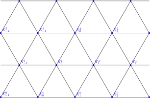
Figure 1: Space-time diagram.

The dependence cone $\mathcal{D}(i,n)$ of the variable $X^{n}_{i}$ is defined as the set of variables which are influenced by the value of $X^{n}_{i}$. If the neighborhood is $\mathcal{N}=\{0,\dots\ell\}$, then $\mathcal{D}(i,n)=\{X^{n+k}_{i+j},k\in\mathbb{N},-k\ell\leq j\leq 0\}.$

Next lemma follows directly from the definition of a PCA.

Lemma 2.2.

Let $(i,n)$ belong to $\mathbb{Z}\times(\mathbb{N}\setminus\{0\})$ and let $S$ be a subset of $\mathbb{Z}\times\mathbb{N}$ such that $\mathcal{D}(i,n)\cap S=\emptyset$. Then, $X^{n}_{i}$ is independent of $(X^{m}_{j})_{(j,m)\in S}$ conditionally to $(X^{n-1}_{i+v})_{v\in\mathcal{N}}$.

We point out that if a PCA has positive rates, i.e., $\forall u\in\mathcal{A}^{\mathcal{N}},\forall a\in\mathcal{A},\ f(u)(a)>0$, then any of its stationary space-time diagram is a Markovian random field. We refer to [10] for an in-depth study of the connections between Gibbs states and stationary space-time diagrams of PCA.

2.3 Product form invariant measures

Definition 2.3.

For $p\in[0,1]$, we denote by $\mu_{p}$ the Bernoulli product measure of parameter $p$ on $\{0,1\}^{\mathbb{Z}}$, that is, $\mu_{p}={\mathcal{B}}_{p}^{\otimes\mathbb{Z}}$, where ${\mathcal{B}}_{p}$ denotes the Bernoulli measure of parameter $p$ on $\{0,1\}$. Thus, for any cylinder $[x]$, we have

$$\mu_{p}[x]=(1-p)^{|x|_{0}}p^{|x|_{1}}\>.$$

We give a first property of the space-time diagram that is shared by every PCA having a Bernoulli product invariant measure.

Lemma 2.4.

Let $F$ be a PCA of neighborhood $\{0,\ldots,\ell\}$. Assume that $\mu_{p}F=\mu_{p}$ and consider the stationary space-time diagram obtained for that invariant measure. Then for any $\alpha>-1/\ell$, the line $L_{\alpha}=\{(k,n)\in\mathbb{Z}\times\mathbb{N}\mid n=\alpha k\}$ is such that the random variables $(X_{k}^{n})_{(k,n)\in L_{\alpha}}$ are i.i.d.

Proof.

Let us show that any finite sequence of consecutive random variables on such a line is i.i.d. We can assume without loss of generality that the first of these points is $X_{0}^{0}$. Then, using the hypothesis on the slope, we obtain that the other random variables on that line are all outside the dependence cone of $X_{0}^{0}$. Thus, the $(n-1)$-tuple they constitute is independent of $X_{0}^{0}$. By induction, we get the result. ∎

3 PCA of alphabet and neighborhood of size 2

For the time being, we assume that the neighborhood is $\mathcal{N}=\{0,1\}$ and that the alphabet is $\mathcal{A}=\{0,1\}$. For convenience, we introduce the notations: for $x,y\in\mathcal{A}$,

$$\theta_{xy}=\theta^{1}_{xy}=f(x,y)(1),\qquad\theta^{0}_{xy}=f(x,y)(0)=1-\theta_{xy}\>.$$

Observe that a PCA is completely characterized by the four parameters: $\theta_{00},\theta_{01},\theta_{10}$, and $\theta_{11}$.

3.1 Computation of the image of a product measure by a PCA

The goal of this section is to give an explicit description of the measure $\mu_{p}F$, where $\mu_{p}$ is the Bernoulli product measure of parameter $p$, as a function of the parameters $\theta_{00},\theta_{01},\theta_{10},\theta_{11}$.

Let us start with an observation. Consider $(Y_{n})_{n\in\mathbb{Z}}\sim\mu_{p}F$. Clearly, we have: $(Y_{2n})_{n\in\mathbb{Z}}\sim\mu_{p}$ and $(Y_{2n+1})_{n\in\mathbb{Z}}\sim\mu_{p}$. But the two i.i.d. sequences have a complex joint correlation structure. It makes it non-elementary to describe the finite-dimensional marginals of $\mu_{p}F$.

Assume that the parameters satisfy:

$$(\theta_{00},\theta_{01}),(\theta_{10},\theta_{11})\not\in\{(0,0),(1,1)\}\>.$$ (1)

For $p\in(0,1)$, $\alpha\in\{0,1\}$, define the function

$$\begin{array}[]{cccl}g_{\alpha}:&[0,1]&\longrightarrow&(0,1)\\ &q&\longmapsto&(1-q)\;(1-p)\;\theta_{00}^{\alpha}+(1-q)\;p\;\theta_{01}^{\alpha}+q\;(1-p)\;\theta_{10}^{\alpha}+q\;p\;\theta_{11}^{\alpha}\>.\end{array}$$ (2)

Consider three random variables $X_{0},X_{1},Y_{0}$ with $(X_{0},X_{1})\sim{\mathcal{B}}_{q}\otimes{\mathcal{B}}_{p}$ and $Y_{0}\sim({\mathcal{B}}_{q}\otimes{\mathcal{B}}_{p})f$. In words, $g_{\alpha}(q)$ is the probability to have $Y_{0}=\alpha$. With the condition (1), we have $g_{\alpha}(q)\in(0,1)$ for all $q$. Observe also that: $g_{0}(q)+g_{1}(q)=1$ for all $q$.

For $p\in(0,1)$, $\alpha\in\{0,1\}$, we also define the function

$$\begin{array}[]{cccl}h_{\alpha}:&[0,1]&\longrightarrow&[0,1]\\ &q&\longmapsto&\bigl{[}(1-q)\;p\;\theta_{01}^{\alpha}+q\;p\;\theta_{11}^{\alpha}\bigr{]}g_{\alpha}(q)^{-1}\>.\end{array}$$ (3)

Consider $X_{0},X_{1},Y_{0}$ with $(X_{0},X_{1})\sim{\mathcal{B}}_{q}\otimes{\mathcal{B}}_{p}$ and $Y_{0}\sim({\mathcal{B}}_{q}\otimes{\mathcal{B}}_{p})f$. In words, $h_{\alpha}(q)$ is the probability to have $X_{1}=1$ conditionally to $Y_{0}=\alpha$.

Proposition 3.1.

Consider a PCA satisfying (1). Consider $p\in(0,1)$. For $\alpha_{0}\cdots\alpha_{n-1}\in\mathcal{A}^{n}$, the probability of the cylinder $[\alpha_{0}\cdots\alpha_{n-1}]$ under $\mu_{p}F$ is given by:

$$\mu_{p}F[\alpha_{0}\cdots\alpha_{n-1}]=g_{\alpha_{0}}(p)\ \prod_{i=1}^{n-1}g_{\alpha_{i}}(h_{\alpha_{i-1}}(h_{\alpha_{i-2}}(\ldots h_{\alpha_{0}}(p)\ldots)))\>.$$

By reversing the space-direction, we get an analog proposition for a PCA satisfying the symmetrized condition: $(\theta_{00},\theta_{10}),(\theta_{01},\theta_{11})\not\in\{(0,0),(1,1)\}$.

Proof.

Let us compute recursively the value $\mu_{p}F[\alpha_{0}\cdots\alpha_{n-1}]$. We set $X=X^{0}$ and $Y=X^{1}$. Assuming that $X\sim\mu_{p}$, by definition,

$$\mu_{p}F[\alpha_{0}]={\mathbb{P}}(Y_{0}=\alpha_{0})=g_{\alpha_{0}}(p).$$

We can decompose the probability $\mu_{p}F[\alpha_{0}\alpha_{1}]$ into

$$\mu_{p}F[\alpha_{0}\alpha_{1}]={\mathbb{P}}(Y_{0}=\alpha_{0},Y_{1}=\alpha_{1})={\mathbb{P}}(Y_{1}=\alpha_{1}\mid Y_{0}=\alpha_{0})\;{\mathbb{P}}(Y_{0}=\alpha_{0}).$$

By definition, the conditional law of $X_{1}$ assuming that $Y_{0}=\alpha_{0}$ is given by ${\mathcal{B}}_{h_{\alpha_{0}}(p)}$. So the law of $(X_{1},X_{2})$ is ${\mathcal{B}}_{h_{\alpha_{0}}(p)}\otimes{\mathcal{B}}_{p}$ and we obtain

$$\mu_{p}F[\alpha_{0}\alpha_{1}]=g_{\alpha_{1}}(h_{\alpha_{0}}(p))\;g_{\alpha_{0}}(p).$$

More generally, we have:

$${\mathbb{P}}(Y_{0}=\alpha_{0}\ldots Y_{k}=\alpha_{k})={\mathbb{P}}(Y_{k}=\alpha_{k}\mid Y_{0}=\alpha_{0}\ldots Y_{k-1}=\alpha_{k-1})\;{\mathbb{P}}(Y_{0}=\alpha_{0}\ldots Y_{k-1}=\alpha_{k-1}).$$

By induction, the law of $X_{k}$ knowing that $Y_{0}=\alpha_{0}\ldots Y_{k-1}=\alpha_{k-1}$ is ${\mathcal{B}}_{h_{\alpha_{k-1}}(h_{\alpha_{k-2}}(\ldots h_{\alpha_{0}}(p)\ldots))}$. The result follows. ∎

3.2 Conditions for a product measure to be invariant

For $x\in{\mathcal{X}}$, denote by $\delta_{x}$ the Dirac probability measure concentrated on the configuration $x$. The probability measure $\mu_{1}=\delta_{1^{\mathbb{Z}}}$ is invariant for the PCA $F$ if and only if $\theta_{11}=1$. Similarly, $\mu_{0}=\delta_{0^{\mathbb{Z}}}$ is invariant for $F$ if and only if $\theta_{00}=0$.

Using Proposition 3.1, we get a necessary and sufficient condition for $\mu_{p}$, $p\in(0,1)$, to be an invariant measure of $F$. The result is stated in Theorem 3.2. It already appeared in [1] and [12], but our proof is new and simpler.

Theorem 3.2.

The measure $\mu_{p}$, $p\in(0,1)$, is an invariant measure of the PCA $F$ of parameters $\theta_{00},\theta_{01},\theta_{10},\theta_{11}$ if and only if one of the two following conditions is satisfied:

$$(i) (1-p)\;\theta_{00}+p\;\theta_{01}=(1-p)\;\theta_{10}+p\;\theta_{11}=p$$

$$(ii) (1-p)\;\theta_{00}+p\;\theta_{10}=(1-p)\;\theta_{01}+p\;\theta_{11}=p\>.$$

In particular, a PCA has a (non-trivial) Bernoulli product invariant measure if and only if its parameters satisfy:

$$\theta_{00}\;(1-\theta_{11})=\theta_{10}\;(1-\theta_{01})\;\quad\mbox{ or }\quad\;\theta_{00}\;(1-\theta_{11})=\theta_{01}\;(1-\theta_{10})\>.$$ (4)

Proof.

Let us assume that $F$ satisfies condition (i) for some $p\in(0,1)$. Then, the function $g_{1}$ is given by $g_{1}(q)=(1-q)\;p+q\;p=p$, and $g_{0}(q)=1-g_{1}(q)=1-p$. By Proposition 3.1, we have,

$$\forall\alpha=\alpha_{0}\cdots\alpha_{n-1}\in\mathcal{A}^{n},\quad\mu_{p}F[\alpha]=(1-p)^{|\alpha|_{0}}p^{|\alpha|_{1}}=\mu_{p}[\alpha]\>.$$

So $\mu_{p}$ is an invariant measure.

Now, assume that the PCA $F$ satisfies condition (ii). Let us reverse the space direction, that is, let us read the configurations from right to left. The same dynamic is now described by a new PCA $\widetilde{F}$ defined by the parameters $\tilde{\theta}_{00}=\theta_{00},\tilde{\theta}_{01}=\theta_{10},\tilde{\theta}_{10}=\theta_{01},\tilde{\theta}_{11}=\theta_{11}$. So, the new PCA satisfies condition $(i)$. According to the above, we have $\mu_{p}\widetilde{F}=\mu_{p}$. Let us reverse the space direction, once again. Since the Bernoulli product measure is unchanged, we obtain $\mu_{p}F=\mu_{p}$.

Conversely, assume that $\mu_{p}F=\mu_{p}$. It follows from Proposition 3.1 that for any value of the $\alpha_{i}$, we must have $g_{1}(h_{\alpha_{n-1}}(h_{\alpha_{n-2}}(\ldots h_{\alpha_{0}}(p)\ldots)))=p$. Since $g_{1}$ is an affine function, there are only two possibilities: either $g_{1}$ is the constant function equal to $p$; or $h_{\alpha_{n-1}}(h_{\alpha_{n-2}}(\ldots h_{\alpha_{0}}(p)\ldots)))=p$ for all values of $\alpha_{0},\ldots,\alpha_{n-1}\in\mathcal{A}$.

In the first case, observe that

$$g_{1}(q)=q\;[-(1-p)\;\theta_{00}-p\;\theta_{01}+(1-p)\;\theta_{10}+p\;\theta_{11}]+(1-p)\;\theta_{00}+p\;\theta_{01}\>.$$

To get: $\forall q\in[0,1],\ g_{1}(q)=p$, we must have condition (i).

In the second case, we must have $h_{0}(p)=h_{1}(p)=p$ and $g_{1}(p)=p$. Using $g_{0}(p)=1-p$ and $g_{1}(p)=p$, we get:

$$h_{0}(p) = \bigl{[}(1-p)\;p\;(1-\theta_{01})+p\;p\;(1-\theta_{11})\bigr{]}(1-p)^{-1}$$

$$h_{1}(p) = \bigl{[}(1-p)\;p\;\theta_{01}+p\;p\;\theta_{11}\bigr{]}p^{-1}\ =\ (1-p)\;\theta_{01}+p\;\theta_{11}\>.$$

The equality $h_{1}(p)=p$ provides the condition $(1-p)\;\theta_{01}+p\;\theta_{11}=p$. Let us switch to the equality $h_{0}(p)=p$. We have:

$$h_{0}(p)=p \iff (1-p)\;(1-\theta_{01})+p\;(1-\theta_{11})=1-p$$

$$\iff (1-p)\;\theta_{01}+p\;\theta_{11}=p\>.$$

So, we obtain condition (ii). ∎

To complete Theorem 3.2, let us quote a result from [13]. We recall that a PCA has positive rates if: $\forall u\in\mathcal{N},\forall a\in\mathcal{A},\ f(u)(a)>0$.

Proposition 3.3.

Consider a positive-rates PCA $F$ satisfying condition $(i)$ or $(ii)$, for some $p\in(0,1)$. Then $F$ is ergodic, that is, $\mu_{p}$ is the unique invariant measure of $F$ and for all initial measure $\mu$, the sequence $(\mu F^{n})_{n\geq 0}$ converges weakly to $\mu_{p}$.

Assessing the ergodicity of a PCA is a difficult problem, which is algorithmically undecidable in general, see [11, 3]. On the other hand, a long standing conjecture had been that any PCA with positive rates is ergodic. However, in 2001, Gács disproved the conjecture by exhibiting a very complex counter-example with several invariant measures [5]. In this complicated landscape, Proposition 3.3 gives a restricted setting in which ergodicity can be proven.

Observe that Proposition 3.3 is not true without the positive-rates assumption. Consider for instance the PCA defined by: $\theta_{00}=p/(1-p),\theta_{01}=0,\theta_{10}=0,\theta_{11}=1$ for some $p\in(0,1/2]$. It satisfies $(i)$ and $(ii)$, but it is not ergodic since $\delta_{1^{\mathbb{Z}}}$ and $\mu_{p}$ are both invariant.

3.3 Transversal PCA

We assume that $\mu_{p}$ is invariant under the action of the PCA, and we focus on the correlation structure of the space-time diagram obtained when the initial measure is $\mu_{p}$. Observe that this space-time diagram is both space-stationary and time-stationary. By time-stationarity, the space-time diagram can be extended from $\mathbb{Z}\times\mathbb{N}$ to $\mathbb{Z}^{2}$. From now on, we work with this extension.

Let $(X_{k,n})_{k,n\in\mathbb{Z}\times\mathbb{Z}}$ be a realization of the stationary space-time diagram.

It is convenient to define the three vectors $\vec{u},\vec{v},$ and $\vec{w}$ as in the figure above. The PCA generating the space-time diagram is the PCA of direction $\vec{u}$. In some cases, the space-time diagram when rotated by an angle of $2\pi/3$ (resp. $-2\pi/3$) still has the correlation structure of a space-time diagram generated by a PCA of neighborhood $\{0,1\}$. In this case, we say that, in the original space-time diagram, there is a transversal PCA of direction $\vec{v}$ (resp. $\vec{w}$).

Proposition 3.4.

Under condition (i), each line of angle $\pi/3$ of the space-time diagram is distributed according to $\mu_{p}$. Moreover, their correlations are the ones of a transversal PCA of direction $\vec{v}$ and rates given by: $\vartheta_{00}=\theta_{00}$, $\vartheta_{01}=\theta_{10}$, $\vartheta_{10}=\theta_{01}$, $\vartheta_{11}=\theta_{11}$.

To prove Prop. 3.4, we need two preliminary lemmas. Set $X=X^{0}$ and $Y=X^{1}$, so that we have in particular $(X,Y)\sim(\mu_{p},\mu_{p}F)$.

Lemma 3.5.

Under condition (i), the variables $(Y_{k})_{k\geq 0}$ are independent of $X_{0}$, that is, for any $n\geq 0$,

$${\mathbb{P}}\bigl{(}X_{0}=x_{0},(Y_{i})_{0\leq i\leq n}=(y_{i})_{0\leq i\leq n}\bigr{)}=\mu_{p}[x_{0}]\prod_{i=0}^{n}\mu_{p}[y_{i}]\>.$$

Proof.

The left-hand side can be decomposed into:

$$\sum_{x_{1}\cdots x_{n+1}\in\{0,1\}^{n+1}}{\mathbb{P}}\bigl{(}(X_{i})_{0\leq i\leq n+1}=(x_{i})_{0\leq i\leq n+1},(Y_{i})_{0\leq i\leq n}=(y_{i})_{0\leq i\leq n}\bigr{)},$$

which can be expressed with the transition rates of the PCA as follows:

$$\sum_{x_{1}\cdots x_{n+1}\in\{0,1\}^{n+1}}\mu_{p}[x_{0}]\prod_{i=0}^{n}\mu_{p}[x_{i+1}]\theta_{x_{i}x_{i+1}}^{y_{i}}$$

$$=\mu_{p}[x_{0}]\sum_{x_{1}\in\{0,1\}}\mu_{p}[x_{1}]\theta_{x_{0}x_{1}}^{y_{0}}\sum_{x_{2}\in\{0,1\}}\mu_{p}[x_{2}]\theta_{x_{1}x_{2}}^{y_{1}}\ \cdots\ \sum_{x_{n+1}\in\{0,1\}}\mu_{p}[x_{n+1}]\theta_{x_{n}x_{n+1}}^{y_{n}}.$$

Condition ${\it(i)}$ can be rewritten as:

$$\forall a,b,c\in\{0,1\},\qquad\sum_{b\in\{0,1\}}\mu_{p}[b]\theta_{ab}^{c}=\mu_{p}[c]\>.$$

Using this, and simplifying from the right to the left, we obtain: $\mu_{p}[x_{0}]\prod_{i=0}^{n}\mu_{p}[y_{i}]$.∎

Lemma 3.6.

Under condition (i), for any $n\geq 0$,

$${\mathbb{P}}(X_{0}=x_{0},X_{1}=x_{1},(Y_{i})_{0\leq i\leq n}=(y_{i})_{0\leq i\leq n})=\mu_{p}[x_{0}]\mu_{p}[x_{1}]\theta_{x_{0}x_{1}}^{y_{0}}\prod_{i=1}^{n}\mu_{p}[y_{i}]\>.$$

Proof.

The proof is analogous. We decompose the left-hand side into:

$$\sum_{x_{2}\cdots x_{n+1}\in\{0,1\}^{n}}{\mathbb{P}}((X_{i})_{0\leq i\leq n+1}=(x_{i})_{0\leq i\leq n+1},(Y_{i})_{0\leq i\leq n}=(y_{i})_{0\leq i\leq n}),$$

which can be expressed with the transition rates of the PCA as follows:

$$\sum_{x_{2}\cdots x_{n+1}\in\{0,1\}^{n}}\mu_{p}[x_{0}]\prod_{i=0}^{n}\mu_{p}[x_{i+1}]\theta_{x_{i}x_{i+1}}^{y_{i}}$$

$$=\mu_{p}[x_{0}]\mu_{p}[x_{1}]\theta_{x_{0}x_{1}}^{y_{0}}\sum_{x_{2}\in\{0,1\}}\mu_{p}[x_{2}]\theta_{x_{1}x_{2}}^{y_{1}}\ldots\sum_{x_{n+1}\in\{0,1\}}\mu_{p}[x_{n+1}]\theta_{x_{n}x_{n+1}}^{y_{n}}.$$

Using ${\it(i)}$ and simplifying from the right to the left, we get the result. ∎

Proof of Proposition 3.4..

To prove the first part of the proposition, it is sufficient to prove that the sequence $(X_{0}^{k})_{k\in\mathbb{Z}}$ is i.i.d. For a given $n\in\mathbb{N}$ and a sequence $(\alpha_{k})_{0\leq k\leq n}$, let us prove recursively that ${\mathbb{P}}((X_{0}^{n})_{0\leq k\leq n}=(\alpha_{k})_{0\leq k\leq n})=\mu_{p}[\alpha_{0}\cdots\alpha_{n}].$ For $n=0$, the result is straightforward; and for $n=1$, it is a direct consequence of Lemma 3.5. For larger values of $n$, set $A={\mathbb{P}}((X_{0}^{k})_{0\leq k\leq n}=(\alpha_{k})_{0\leq k\leq n})$, we have:

$$A\ =\sum_{y_{1}\cdots y_{n-1}\in\{0,1\}^{n-1}}{\mathbb{P}}\bigl{(}(X_{0}^{k})_{0\leq k\leq n}=(\alpha_{k})_{0\leq k\leq n},(Y_{i})_{1\leq i\leq n-1}=(y_{i})_{1\leq i\leq n-1}\bigr{)}\>.$$

Since $X^{0}_{0}=X_{0},X_{0}^{1}=Y_{0}$, it can be rewritten as:

$$A = \sum_{y_{1}\cdots y_{n-1}\in\{0,1\}^{n-1}}{\mathbb{P}}\bigl{(}(X_{0}^{k})_{2\leq k\leq n}=(\alpha_{k})_{2\leq k\leq n}\mid X_{0}=\alpha_{0},Y_{0}=\alpha_{1},(Y_{i})_{1\leq i\leq n-1}=(y_{i})_{1\leq i\leq n-1}\bigl{)}$$

$$\qquad\qquad\qquad\qquad\times\;{\mathbb{P}}\bigl{(}X_{0}=\alpha_{0},Y_{0}=\alpha_{1},(Y_{i})_{1\leq i\leq n-1}=(y_{i})_{1\leq i\leq n-1}\bigl{)}\>.$$

The law of $(X_{0}^{k})_{2\leq k\leq n}$ conditionally to $(X_{0},(Y_{i})_{0\leq i\leq n-1})$ is equal to the law of $(X_{0}^{k})_{2\leq k\leq n}$ conditionally to $(Y_{i})_{0\leq i\leq n-1}$. Also, using Lemma 3.5, we have: ${\mathbb{P}}\bigl{(}X_{0}=\alpha_{0},Y_{0}=\alpha_{1},(Y_{i})_{1\leq i\leq n-1}=(y_{i})_{1\leq i\leq n-1}\bigl{)}=\mu_{p}[\alpha_{0}]\;{\mathbb{P}}(Y_{0}=\alpha_{1},(Y_{i})_{1\leq i\leq n-1}=(y_{i})_{1\leq i\leq n-1})$. Coupling these two points, we get:

$$A = \sum_{y_{1}\cdots y_{n-1}\in\{0,1\}^{n-1}}{\mathbb{P}}\bigl{(}(X_{0}^{k})_{2\leq k\leq n}=(\alpha_{k})_{2\leq k\leq n}\mid Y_{0}=\alpha_{1},(Y_{i})_{1\leq i\leq n-1}=(y_{i})_{1\leq i\leq n-1}\bigl{)}$$

$$\qquad\qquad\qquad\qquad\times\;\mu_{p}[\alpha_{0}]\;{\mathbb{P}}(Y_{0}=\alpha_{1},(Y_{i})_{1\leq i\leq n-1}=(y_{i})_{1\leq i\leq n-1})$$

$$= \mu_{p}[\alpha_{0}]\;{\mathbb{P}}\bigl{(}(X_{0}^{k})_{1\leq k\leq n}=(\alpha_{k})_{1\leq k\leq n}\bigr{)}\>.$$

By induction, we obtain the result.

The second part of the proposition consists in proving that

$${\mathbb{P}}\bigl{(}(X^{k}_{1})_{0\leq k\leq n}=(\beta_{k})_{0\leq k\leq n}\mid(X^{k}_{0})_{0\leq k\leq n+1}=(\alpha_{k})_{0\leq k\leq n+1}\bigr{)}=\prod_{k=0}^{n}\vartheta_{\alpha_{k+1}\alpha_{k}}^{\beta_{k}}\>.$$ (5)

We prove the result recursively. For $n=0$, set $A={\mathbb{P}}(X_{1}=\beta_{0}\mid Y_{0}=\alpha_{1},X_{0}=\alpha_{0})$. We want to prove that $A=\vartheta^{\beta_{0}}_{\alpha_{1}\alpha_{0}}$. Using the first part of the proposition, we have:

$$A = {\mathbb{P}}(Y_{0}=\alpha_{1}\mid X_{0}=\alpha_{0},X_{1}=\beta_{0})\;{\mathbb{P}}(X_{0}=\alpha_{0},X_{1}=\beta_{0})\;{\mathbb{P}}(X_{0}=\alpha_{0},Y_{0}=\alpha_{1})^{-1}$$

$$= \theta^{\alpha_{1}}_{\alpha_{0}\beta_{0}}\;\mu_{p}[\alpha_{0}]\;\mu_{p}[\beta_{0}]\;\mu_{p}[\alpha_{0}]^{-1}\;\mu_{p}[\alpha_{1}]^{-1}\quad=\quad\theta^{\alpha_{1}}_{\alpha_{0}\beta_{0}}\;\mu_{p}[\beta_{0}]\;\mu_{p}[\alpha_{1}]^{-1}\>.$$

If $\alpha_{1}=\beta_{0}=u$, we get $A=\theta^{u}_{\alpha_{0}u}=\vartheta^{u}_{u\alpha_{0}}$. Assume that $\alpha_{1}\not=\beta_{0}$. Condition $(i)$ can be rewritten as:

$$\mu_{p}[\beta_{0}]\;\theta^{\alpha_{1}}_{\alpha_{0}\beta_{0}}+\mu_{p}[\alpha_{1}]\;\theta^{\alpha_{1}}_{\alpha_{0}\alpha_{1}}=\mu_{p}[\alpha_{1}]\>.$$ (6)

Dividing by $\mu_{p}[\alpha_{1}]$, we get:

$$A=\theta^{\alpha_{1}}_{\alpha_{0}\beta_{0}}\;\mu_{p}[\beta_{0}]\;\mu_{p}[\alpha_{1}]^{-1}=1-\theta^{\alpha_{1}}_{\alpha_{0}\alpha_{1}}=\theta^{\beta_{0}}_{\alpha_{0}\alpha_{1}}=\vartheta^{\beta_{0}}_{\alpha_{1}\alpha_{0}}\>.$$

For larger $n$, it is convenient to prove next equality, which is equivalent to (5):

$${\mathbb{P}}\bigl{(}(X^{k}_{0})_{0\leq k\leq n+1}=(\alpha_{k})_{0\leq k\leq n+1},(X^{k}_{1})_{0\leq k\leq n}=(\beta_{k})_{0\leq k\leq n}\bigr{)}\ =\ \mu_{p}[\alpha_{n+1}]\prod_{k=0}^{n}\mu_{p}[\alpha_{k}]\vartheta_{\alpha_{k+1}\alpha_{k}}^{\beta_{k}}.$$

The left-hand side can be decomposed into:

$$\sum_{y_{2}\cdots y_{n}\in\{0,1\}^{n-1}}{\mathbb{P}}\bigl{(}(X^{k}_{0})_{0\leq k\leq n+1}=(\alpha_{k})_{0\leq k\leq n+1},(X^{k}_{1})_{0\leq k\leq n}=(\beta_{k})_{0\leq k\leq n},(Y_{i})_{2\leq i\leq n}=(y_{i})_{2\leq i\leq n}\bigr{)}\>.$$

Let us decompose each term of the sum, conditioning by the values of $X_{0},X_{1},Y_{0},$ and $Y_{1}$. We have:

$${\mathbb{P}}\bigl{(}(X^{k}_{0})_{2\leq k\leq n+1}=(\alpha_{k})_{2\leq k\leq n+1},(X^{k}_{1})_{2\leq k\leq n}=(\beta_{k})_{2\leq k\leq n}\mid(X_{0},X_{1},Y_{0},Y_{1})=(\alpha_{0},\beta_{0},\alpha_{1},\beta_{1}),(Y_{i})_{2\leq i\leq n}=(y_{i})_{2\leq i\leq n}\bigr{)}$$

$$={\mathbb{P}}\bigl{(}(X^{k}_{0})_{2\leq k\leq n+1}=(\alpha_{k})_{2\leq k\leq n+1},(X^{k}_{1})_{2\leq k\leq n}=(\beta_{k})_{2\leq k\leq n}\mid(Y_{0},Y_{1})=(\alpha_{1},\beta_{1}),(Y_{i})_{2\leq i\leq n}=(y_{i})_{2\leq i\leq n}\bigr{)}\>.$$

and using Lemma 3.6, and the equality $\mu_{p}[\beta_{0}]\theta_{\alpha_{0}\beta_{0}}^{\alpha_{1}}=\mu_{p}[\alpha_{1}]\vartheta_{\alpha_{1}\alpha_{0}}^{\beta_{0}}$ (see (6)):

$${\mathbb{P}}\bigl{(}(X_{0},X_{1},Y_{0},Y_{1})=(\alpha_{0},\beta_{0},\alpha_{1},\beta_{1}),(Y_{i})_{2\leq i\leq n}=(y_{i})_{2\leq i\leq n}\bigr{)}\qquad\qquad\qquad$$

$$= \mu_{p}[\alpha_{0}]\mu_{p}[\beta_{0}]\theta_{\alpha_{0}\beta_{0}}^{\alpha_{1}}\;{\mathbb{P}}\bigl{(}Y_{1}=\beta_{1},(Y_{i})_{2\leq i\leq n}=(y_{i})_{2\leq i\leq n}\bigr{)}$$

$$= \mu_{p}[\alpha_{0}]\mu_{p}[\alpha_{1}]\vartheta_{\alpha_{1}\alpha_{0}}^{\beta_{0}}\;{\mathbb{P}}\bigl{(}Y_{1}=\beta_{1},(Y_{i})_{2\leq i\leq n}=(y_{i})_{2\leq i\leq n}\bigr{)}$$

$$= \mu_{p}[\alpha_{0}]\vartheta_{\alpha_{1}\alpha_{0}}^{\beta_{0}}\;{\mathbb{P}}\bigl{(}(Y_{0},Y_{1})=(\alpha_{1},\beta_{1}),(Y_{i})_{2\leq i\leq n}=(y_{i})_{2\leq i\leq n}\bigr{)}\>.$$

Assembling the pieces together, we obtain:

$${\mathbb{P}}\bigl{(}(X^{k}_{0})_{0\leq k\leq n+1}=(\alpha_{k})_{0\leq k\leq n+1},(X^{k}_{1})_{0\leq k\leq n}=(\beta_{k})_{0\leq k\leq n}\bigr{)}$$

$$=\mu_{p}[\alpha_{0}]\vartheta_{\alpha_{1}\alpha_{0}}^{\beta_{0}}\;{\mathbb{P}}\bigl{(}(X^{k}_{0})_{1\leq k\leq n+1}=(\alpha_{k})_{1\leq k\leq n+1},(X^{k}_{1})_{1\leq k\leq n}=(\beta_{k})_{1\leq k\leq n}\bigr{)}\>.$$

We conclude the proof by induction. ∎

Corollary 3.7.

Under condition (i), all the lines of the space-time diagram except possibly those of angle $2\pi/3$ consist of i.i.d. random variables.

Proof.

The previous proposition claims that the lines of angle $\pi/3$ are i.i.d. Lemma 2.4 provides the result for the lines of angle in $[0,\pi/3)\cup(2\pi/3,\pi]$. The angles in $(\pi/3,2\pi/3)$ correspond to lines that are outside the dependence cones of the transversal PCA, so we obtain the result by applying again Lemma 2.4 for the transversal PCA. ∎

In the same way, one can prove the following.

Proposition 3.8.

Under condition (ii), the lines of angle $2\pi/3$ of the space-time diagram are distributed according to $\mu_{p}$ and their correlations are those of a transversal PCA of direction $\vec{w}$ and rates given by $\vartheta_{00}=\theta_{00}$, $\vartheta_{11}=\theta_{11}$ and $\vartheta_{01}=\theta_{10}$, $\vartheta_{10}=\theta_{01}$.

Corollary 3.9.

Under condition (ii), all the lines of the space-time diagram except possibly the ones of angle $\pi/3$ consist of i.i.d. random variables.

For a PCA satisfying (i) (resp. (ii)), the lines of angle $2\pi/3$ (resp. $\pi/3$) are not i.i.d., except if the PCA also satisfies condition (ii) (resp. (i)). The distribution of the lines of angle $2\pi/3$ (resp. $\pi/3$) does not necessary have a Markovian form either. For example, if $\theta_{00}=\theta_{01}=1/2$ and $\theta_{10}=0,\theta_{11}=1$ (condition (i) is satisfied with $p=1/2$), one can check that ${\mathbb{P}}(X_{0}^{0}=0,X_{-1}^{1}=0,X_{-2}^{2}=0)=19/64$ which is different ${\mathbb{P}}(X_{0}^{0}=0){\mathbb{P}}(X_{-1}^{1}=0\mid X_{0}^{0}=0){\mathbb{P}}(X_{-2}^{2}=0\mid X_{-1}^{1}=0)=(1/2)(3/4)^{2}$.

It is an open problem to know if under condition (i) (resp. (ii)), it is possible to give an explicit description of the distribution of the lines of angle $2\pi/3$ (resp. $\pi/3$).

4 Non-i.i.d. random field with every line i.i.d.

We now concentrate on PCA satisfying both conditions $(i)$ and $(ii)$ for some $p\in(0,1)$. We consider the stationary space-time diagram associated with $\mu_{p}$, and we still denote it by $(X^{n}_{k})_{k,n\in\mathbb{Z}}$.

4.1 All the lines are i.i.d.

For a given $p\in(0,1)$, conditions (i) and (ii) are both satisfied if and only if:

$$\exists s\in\Bigl{[}\frac{2p-1}{p},\frac{p}{1-p}\Bigr{]},\qquad\theta_{00}=\frac{p(1-s)}{1-p},\ \theta_{01}=\theta_{10}=s,\ \theta_{11}=1-\frac{(1-p)s}{p}\>.$$ (7)

Example 4.1.

For any value of $p\in(0,1)$, the choice $s=p$ is allowed. In that case, the transition rates $\theta_{ij}$ are all equal to $p$ and the stationary random field is i.i.d., there is no dependence in the space-time diagram.

Example 4.2.

If $p=1/2$, every choice of $s\in[0,1]$ is valid and the corresponding PCA has the transition function $f(x,y)=s\;\delta_{x+y\mathop{\rm mod}\nolimits 2}+(1-s)\;\delta_{x+y+1\mathop{\rm mod}\nolimits 2}$.

An example of space-time diagram for $p=1/2$ and $s=3/4$

Example 4.3.

For any value of $p\in(0,1/2]$, it is possible to set $s=0$ and then, $\theta_{01}=\theta_{10}=0,\theta_{11}=1$, and $\theta_{00}=p/(1-p)$. This PCA forbids the elementary triangles pointing up that have exactly one vertex labeled by a $0$.

An example of space-time diagram for $p=1/3$ and $s=0$

Next proposition is a direct consequence of Corollaries 3.7 and 3.9.

Proposition 4.4.

Consider a PCA satisfying (7). Every line of the stationary space-time diagram consists of i.i.d. random variables. In particular, any two different variables are independent.

4.2 Equilateral triangles pointing up are correlated

We have seen that all the lines of the space-time diagram are i.i.d. But the whole space-time diagram is i.i.d. if and only if $s=p$. Indeed, if $s\neq p$, the random variable $X^{n+1}_{k}$ is not independent of $(X^{n}_{k},X^{n}_{k+1})$; in words, the three variables of an elementary triangle pointing up are correlated. Precisely, the triple $(X^{n}_{k},X^{n}_{k+1},X^{n+1}_{k})$ consists of random variables which are: (1) identically distributed; (2) pairwise independent; (3) globally dependent if $s\neq p$. The “converse” holds.

Proposition 4.5.

Let $\nu$ be a law on $\{0,1\}^{3}$ such that the three marginals on $\{0,1\}^{2}$ are i.i.d. Assume that $\nu$ is non degenerated ($\nu\neq\delta_{000},\nu\neq\delta_{111}$). Then $\nu$ can be realized as the law of an “elementary triangle pointing up” in the stationary space-time diagram of exactly one PCA satisfying (7).

Proof.

Consider $(X_{0},X_{1},Y_{0})\sim\nu$. Assume that the common law of $X_{0},X_{1},$ and $Y_{0}$ is ${\mathcal{B}}_{p}$. By the pairwise independence, we have:

$${\mathbb{P}}(X_{0}=1,X_{1}=0,Y_{0}=0) = {\mathbb{P}}(X_{1}=0,Y_{0}=0)-{\mathbb{P}}(X_{0}=0,X_{1}=0,Y_{0}=0)$$

$$= (1-p)^{2}-{\mathbb{P}}(X_{0}=0,X_{1}=0,Y_{0}=0)\>.$$

We obtain:

$${\mathbb{P}}(X_{0}=1,X_{1}=0,Y_{0}=0)={\mathbb{P}}(X_{0}=0,X_{1}=1,Y_{0}=0)={\mathbb{P}}(X_{0}=0,X_{1}=0,Y_{0}=1)$$

$${\mathbb{P}}(X_{0}=0,X_{1}=1,Y_{0}=1)={\mathbb{P}}(X_{0}=1,X_{1}=0,Y_{0}=1)={\mathbb{P}}(X_{0}=1,X_{1}=1,Y_{0}=0)\>.$$

Set $q_{0}={\mathbb{P}}(X_{0}=1,X_{1}=0,Y_{0}=0)$ and $q_{1}={\mathbb{P}}(X_{0}=0,X_{1}=1,Y_{0}=1)$. We have:

$${\mathbb{P}}(X_{0}=0,X_{1}=0,Y_{0}=0)=(1-p)^{2}-q_{0},\qquad{\mathbb{P}}(X_{0}=1,X_{1}=1,Y_{0}=1)=p^{2}-q_{1}\>.$$

Furthermore:

$$q_{0}+q_{1}={\mathbb{P}}(X_{0}=0,X_{1}=0,Y_{0}=1)+{\mathbb{P}}(X_{0}=1,X_{1}=0,Y_{0}=1)={\mathbb{P}}(X_{1}=0,Y_{0}=1)=p(1-p)\>.$$

Using the above, and expressing everything as a function of $p$ and $q_{1}$, we get:

$${\mathbb{P}}(Y_{0}=1\mid X_{0}=0,X_{1}=0) = (p(1-p)-q_{1})/(1-p)^{2}$$

$${\mathbb{P}}(Y_{0}=1\mid X_{0}=0,X_{1}=1) = q_{1}/(p(1-p))$$

$${\mathbb{P}}(Y_{0}=1\mid X_{0}=1,X_{1}=0) = q_{1}/(p(1-p))$$

$${\mathbb{P}}(Y_{0}=1\mid X_{0}=1,X_{1}=1) = 1-q_{1}/p^{2}\>.$$

By setting $\theta_{ij}={\mathbb{P}}(Y_{0}=1\mid X_{0}=i,X_{1}=j)$ and $s=q_{1}/(p(1-p))$, we recover exactly (7). ∎

Proposition 4.6.

Consider a PCA satisfying (7) with $s\neq p$. The correlations between three random variables that form an equilateral triangle pointing up decrease exponentially in function of the size of the triangle.

Proof.

Let us consider the random field $(X_{2k}^{2n})_{k,n\in\mathbb{Z}}$. Observe that all its random variables are distributed according to ${\mathcal{B}}_{p}$, and that each line consists of i.i.d. random variables. Moreover, for any $a<b$, the variables $(X^{2n+2}_{2k})_{a\leq k\leq b}$ are independent conditionally to the variables $(X^{2n}_{2k})_{a\leq k\leq b+1}$. Thus, this “extracted” random field corresponds to the space-time diagram of a new PCA, having a neigborhood of size $2$ and satisfying (7) for the same value of $p$. To know its transition rates $\theta^{(2)}_{ij}={\mathbb{P}}(X_{0}^{2}=1\mid X_{0}^{0}=i,X_{2}^{0}=j)$, it is enough to compute $\theta^{(2)}_{10}=\theta^{(2)}_{01}$. We denote this value by $\phi(s)$, since it is a function of $s=\theta_{01}=\theta_{10}$.

Summing on all possible values of $X_{1}^{0},X^{1}_{0},X^{1}_{1}$ (we first consider the case $X_{1}^{0}=1$ and then the one $X_{1}^{0}=0$), we get:

$$\phi(s)=p\;[\theta_{01}\theta_{11}\;\theta_{11}+(1-\theta_{01})\theta_{11}\;\theta_{01}+\theta_{01}(1-\theta_{11})\;\theta_{10}+(1-\theta_{01})(1-\theta_{11})\;\theta_{00}]$$

$$+(1-p)\;[\theta_{00}\theta_{01}\;\theta_{11}+(1-\theta_{00})\theta_{01}\;\theta_{01}+\theta_{00}(1-\theta_{01})\;\theta_{10}+(1-\theta_{00})(1-\theta_{01})\;\theta_{00}].$$

Replacing the coefficients $\theta_{ij}$ by their expression in function of $p$ and $s$ and simplifying the result, we obtain:

$$\phi(s)=p+{(s-p)^{3}\over p(1-p)}.$$

We proceed similarly for the random field $(X_{2^{i}k}^{2^{i}n})_{k,n\in\mathbb{Z}}$. The coefficient $\theta^{(2^{i})}_{01}={\mathbb{P}}(X_{0}^{2^{i}}=1\mid X_{0}^{0}=0,X_{2^{i}}^{0}=1)$ is equal to $\phi^{i}(s)$, which satisfies:

$$\phi^{i}(s)-p={(s-p)^{3^{i}}\over(p(1-p))^{{3^{i}-1\over 2}}}=\sqrt{p(1-p)}\Big{(}{s-p\over\sqrt{p(1-p)}}\Big{)}^{3^{i}}\>.$$

Similar computations can be performed for equilateral triangles pointing up of other sizes. The decay of correlation for equilateral triangles pointing up is exponential in function of their size. ∎

Next lemma will allow us to characterize completely the triples of random variables that are not independent.

Lemma 4.7.

Consider a PCA satisfying (7). The variable $X_{0}^{0}$ is independent of $(X_{k}^{n})_{k\in\mathbb{Z},n\in\mathbb{N}\setminus\{0\}}$.

Proof.

Set $X=X^{0}$ and $Y=X^{1}$. It is sufficient to prove that $X_{0}$ is independent of $(Y_{k})_{k\in\mathbb{Z}}$. But $(Y_{k})_{k\geq 0}$ and $(Y_{k})_{k<0}$ are independent conditionally to $X_{0}$, so that we can conclude with Lemma 3.5 and its analog for condition (ii).∎

Proposition 4.8.

Consider a PCA satisfying (7) with $s\not=p$. Three random variables of the stationary space-time diagram are correlated if and only if they form an equilateral triangle pointing up.

Proof.

Three variables that form an equilateral triangle pointing up are correlated, see the proof of Proposition 4.6. Let us now consider three variables $(Z_{1},Z_{2},Z_{3})$ that do not constitute such a triangle. Then, if we consider the smallest equilateral triangle pointing up that contains them, there is an edge of that triangle that contains exactly one of these variables. By rotation of angle $2\pi/3$ or translation of the diagram, one can assume that this edge is the horizontal one and that it contains the variable $Z_{1}$, and not the variables $Z_{2},Z_{3}$. Now, using Lemma 4.7, we obtain that $Z_{1}$ is independent of $(Z_{2},Z_{3})$. But since $Z_{2}$ and $Z_{3}$ are independent, the three variables $(Z_{1},Z_{2},Z_{3})$ are independent. ∎

There are subsets of four variables that do not contain equilateral triangles pointing up and that are correlated. It is the case in general of $(X_{0},X_{2},Y_{0},Y_{1})$. Let us consider for instance the PCA of Example 4.3. The event $(X_{0},X_{2},Y_{0},Y_{1})=(0,1,1,1)$ has probability zero, since whatever the value of $X_{1}$, the space-time diagram would have an elementary triangle pointing up with exactly one zero.

4.3 Incremental construction of the random field

Let us show how to construct incrementally the stationary space-time diagram of a PCA satisfying conditions (i) and (ii), using two elementary operations.

Consider a PCA satisfying (i) and (ii) for some $p\in(0,1)$. Let $S\subset\mathbb{Z}^{2}$ be the finite set of points of the space-time diagram that has been constructed at some step. Initially $S=\{(0,0)\}$ and $X_{0}^{0}\sim{\mathcal{B}}_{p}$.

• If $(i,n),(i+1,n)\in S,(i,n+1)\not\in S$, and $\mathcal{D}(i,n+1)\cap S=\emptyset$. Choose $X_{i}^{n+1}$ knowing $(X_{i}^{n},X_{i+1}^{n})$ according to the law of the PCA.

  If $(i,n),(i,n+1)\in S,(i+1,n)\not\in S$, and if no point of the dependence cone of $(i+1,n)$ with respect to the transversal PCA of direction $\vec{v}$ belongs to $S$: choose $X_{i+1}^{n}$ knowing $(X_{i}^{n+1},X_{i}^{n})$ according to the law of the transversal PCA of direction $\vec{v}$.

  If $(i,n+1),(i+1,n)\in S,(i,n)\not\in S$, and if no point of the dependence cone of $(i,n)$ with respect to the transversal PCA of direction $\vec{w}$ belongs to $S$: choose $X_{i}^{n}$ knowing $(X_{i+1}^{n},X_{i}^{n+1})$ according to the law of the transversal PCA of direction $\vec{w}$.

• If $(i,n)\not\in S$, and if $(j,m)\in S$ implies $m<n$: choose $X_{i}^{n}$ according to ${\mathcal{B}}_{p}$ and independently of the variables $X_{j}^{m},(j,m)\in S$.

  If $(i,n)\not\in S$, and if $(j,m)\in S$ implies $j<i$: choose $X_{i}^{n}$ according to ${\mathcal{B}}_{p}$ and independently of the variables $X_{j}^{m},(j,m)\in S$.

  If $(i,n)\not\in S$, and if $(j,m)\in S$ implies $j+m>i+n$: choose $X_{i}^{n}$ according to ${\mathcal{B}}_{p}$ and independently of the variables $X_{j}^{m},(j,m)\in S$.

By applying the above rules in the order illustrated by the figure below, one can progressively build the stationary space-time diagram of the PCA. Indeed the rules enlarge $S$ in such a way that, at each step, the variables of $S$ have the same distribution as the corresponding finite-dimensional marginal of the stationary space-time diagram. This is proved by Lemmas 2.2 and 4.7.

On the figure, the labelling of the nodes corresponds to the step at which the corresponding variable is computed (after the three variables of the grey triangle). An arrow pointing to a variable means that it has been constructed according to the PCA of the direction of the arrow (first rule). The nodes labelled by $\amalg$ are the ones which have been constructed by independence (second rule).

5 Extensions

We consider two types of extensions. First, PCA with an alphabet and neighborhood of size 2 but having a Markovian invariant measure. Second, PCA having a Bernoulli product invariant measure but with a general alphabet and neighborhood.

5.1 Markovian invariant measures

Markovian measures are a natural extension of Benoulli product measures. In a nutshell, the tools of Section 3 can be extended to find conditions for having a Markovian invariant measure, but the spatial properties presented in Section 4 do not remain.

Definition 5.1.

Consider $a,b\in(0,1)$. The Markovian measure on $\{0,1\}^{\mathbb{Z}}$ of transition matrix

$$Q=\left(\begin{array}[]{ c c }1-a&a\\ 1-b&b\end{array}\right)$$

is the measure $\nu_{Q}$ defined on cylinders by:

$$\forall x=x_{m}\cdots x_{n},\qquad\nu_{Q}[x]=\pi_{x_{m}}\;\prod_{i=m}^{n-1}Q_{x_{i},x_{i+1}},$$

where $\pi=(\pi_{0},\pi_{1})$ is such that $\pi Q=\pi$, $\pi_{0}+\pi_{1}=1$, that is, $\pi_{0}=(1-b)/(1-b+a)$ and $\pi_{1}=a/(1-b+a)$.

The Markovian measure $\nu_{Q}$ is space-stationary. If $a=b$, then $\nu_{Q}=\mu_{a}$, the Bernoulli product measure of parameter $a$.

Let us fix the PCA, that is, the parameters $(\theta_{00},\theta_{01},\theta_{10},\theta_{11})$ and assume that (1) holds. Let us fix the parameters $a$ and $b$ in $(0,1)$ (defining $Q$ and $\pi$ as in Definition 5.1). We introduce the analogs of the functions defined in (2) and (3).

For $\alpha\in\{0,1\}$, define the function:

$$\begin{array}[]{cccl}g_{\alpha}:&[0,1]&\longrightarrow&(0,1)\\ &r&\longmapsto&(1-r)\;(1-a)\;\theta_{00}^{\alpha}+(1-r)\;a\;\theta_{01}^{\alpha}+r\;(1-b)\;\theta_{10}^{\alpha}+r\;b\;\theta_{11}^{\alpha}\>.\end{array}$$ (8)

In words, $g_{\alpha}(r)$ is the probability that $Y_{0}=\alpha$ if the law of $(X_{0},X_{1})$ is given by ${\mathbb{P}}(X_{0}=x_{0},X_{1}=x_{1})=r_{x_{0}}\;Q_{x_{0},x_{1}}$ with $r_{0}=1-r$ and $r_{1}=r$. With condition (1) on the parameters, we have $g_{\alpha}(r)\in(0,1)$ for all $r$. Observe also that: $g_{0}(r)+g_{1}(r)=1$.

For $\alpha\in\{0,1\}$, we also define the function:

$$\begin{array}[]{cccl}h_{\alpha}:&[0,1]&\longrightarrow&[0,1]\\ &r&\longmapsto&\bigl{[}(1-r)\;a\;\theta_{01}^{\alpha}+r\;b\;\theta_{11}^{\alpha}\bigr{]}g_{\alpha}(r)^{-1}\>.\end{array}$$ (9)

In words, $h_{\alpha}(r)$ is the probability to have $X_{1}=1$ conditionally to $Y_{0}=\alpha$ if $(X_{0},X_{1})$ is distributed according to the above law.

Proposition 5.2.

Consider the Markovian measure $\nu_{Q}$ and the PCA $F$ as above. For $\alpha_{0}\cdots\alpha_{n-1}\in\mathcal{A}^{n}$, the probability of the cylinder $[\alpha_{1}\cdots\alpha_{n}]$ under $\nu_{Q}F$ is given by:

$$\nu_{Q}F[\alpha_{0}\cdots\alpha_{n-1}]=g_{\alpha_{0}}(\pi_{1})\;\prod_{i=1}^{n-1}g_{\alpha_{i}}(h_{\alpha_{i-1}}(h_{\alpha_{i-2}}(\ldots h_{\alpha_{0}}(\pi_{1})\ldots)))\>.$$

Using Proposition 5.2, we obtain sufficient conditions for having a Markovian invariant measure. This provides a new proof of a result mentioned in [12] and first published in [1].

Theorem 5.3.

A PCA has a Markovian invariant measure if its parameters satisfy:

$$\theta_{00}\;\theta_{11}\;(1-\theta_{01})\;(1-\theta_{10})=\theta_{01}\;\theta_{10}\;(1-\theta_{00})\;(1-\theta_{11})\>,$$ (10)

and $(\theta_{00},\theta_{01}),(\theta_{10},\theta_{11})\not\in\{(0,0),(1,1)\}$ or $(\theta_{00},\theta_{10}),(\theta_{01},\theta_{11})\not\in\{(0,0),(1,1)\}$.

Proof.

We treat the case $(\theta_{00},\theta_{01}),(\theta_{10},\theta_{11})\not\in\{(0,0),(1,1)\}$ (for which Prop. 5.2 holds). The case $(\theta_{00},\theta_{10}),(\theta_{01},\theta_{11})\not\in\{(0,0),(1,1)\}$ can be treated by reversing the space-direction.

Let us assume that the following conditions are satisfied:

1. for $\alpha\in\{0,1\}$, $g_{\alpha}(\pi_{1})=\pi_{\alpha}$;

2. for $\alpha\in\{0,1\}$, there exists $c_{\alpha}\in[0,1]$ such that: $\forall r,\ h_{\alpha}(r)=c_{\alpha}$;

3. for $\alpha,\beta\in\{0,1\}$, $g_{\beta}(c_{\alpha})=Q_{\alpha,\beta}$.

Then, by a direct application of Proposition 5.2, the measure $\nu_{Q}$ is invariant. When are these conditions fulfilled?

For $\alpha=1$, condition 2 tells us that there exists $c_{1}\in[0,1]$ such that for any $r\in[0,1]$,

$$(1-r)\;a\;\theta_{01}+r\;b\;\theta_{11}=c_{1}\big{(}(1-r)\;(1-a)\;\theta_{00}+(1-r)\;a\;\theta_{01}+r\;(1-b)\;\theta_{10}+r\;b\;\theta_{11}\big{)}.$$

This is the case if and only if:

$$a\;\theta_{01}=c_{1}((1-a)\;\theta_{00}+a\;\theta_{01}),\qquad b\;\theta_{11}=c_{1}((1-b)\;\theta_{10}+b\;\theta_{11})\>.$$

Thus, condition 2 for $\alpha=1$ is equivalent to:

$$a\;(1-b)\;\theta_{01}\;\theta_{10}=(1-a)\;b\;\theta_{00}\;\theta_{11}\>.$$ (11)

In the same way, condition 2 for $\alpha=0$ is equivalent to:

$$a\;(1-b)\;(1-\theta_{01})\;(1-\theta_{10})=(1-a)\;b\;(1-\theta_{00})\;(1-\theta_{11})\>.$$ (12)

Eliminating $a$ and $b$ in (11) and (12), we obtain the relation (10) for the parameters of the PCA.

Conversely, let us assume that relation (10) holds. We will prove that there exists $a,b\in(0,1)$ such that the three above conditions are satisfied.

First observe that (11) holds if and only if (12) holds. So, we have a first relation to be satisfied by the parameters $a,b\in(0,1)$ which is (11). Under this relation, condition 2 is satisfied with:

$$c_{0}={a\;(1-\theta_{01})\over(1-a)\;(1-\theta_{00})+a\;(1-\theta_{01})}={b\;(1-\theta_{11})\over(1-b)\;(1-\theta_{10})+b\;(1-\theta_{11})}\>,$$ (13)

and

$$c_{1}={a\;\theta_{01}\over(1-a)\;\theta_{00}+a\;\theta_{01}}={b\;\theta_{11}\over(1-b)\;\theta_{10}+b\;\theta_{11}}\>.$$ (14)

Now consider condition 3 for $\alpha=\beta=1$. Symplifying using (14), we obtain:

$$g_{1}(c_{1})=Q_{11}=b\ \iff\ (1-a)\;\theta_{00}=b\;(1-\theta_{11})\>.$$ (15)

Condition 3 for other values of $\alpha$ and $\beta$ provide the same relation after simplification.

Let us show that if equations (11) and (15) are satisfied, then the PCA also fulfills condition 1. Is is sufficient to prove that $g_{1}(\pi_{1})=\pi_{1}$. Expanding both sides of (12) and simplifying using (11), we obtain:

$$a(1-b)\;(1-\theta_{01}-\theta_{10})=(1-a)b\;(1-\theta_{00}-\theta_{11})\>.$$ (16)

Applying the definition (8), we have:

$$g_{1}(\pi_{1})={1\over 1-b+a}\;\Big{(}(1-b)(1-a)\;\theta_{00}+(1-b)a\;\theta_{01}+a(1-b)\;\theta_{10}+ab\;\theta_{11}\Big{)}\>.$$

Using (16), we can replace $a(1-b)(\theta_{01}+\theta_{10})$ by $a(1-b)-(1-a)b\;(1-\theta_{00}-\theta_{11})$. With (15), we finally obtain $g_{1}(\pi_{1})=a/(1-b+a)=\pi_{1}$.

Now, observe that the system:

$$\left\{\begin{array}[]{l}(1-a)\;b\;\theta_{01}\;\theta_{10}=a\;(1-b)\;\theta_{00}\;\theta_{11}\\ (1-a)\;\theta_{00}=b\;(1-\theta_{11})\end{array}\right.$$ (17)

has a unique solution $(a,b)\in(0,1)^{2}$. Let $Q$ be the matrix associated with $(a,b)$. Since the three above conditions are satisfied, the Markovian measure $\nu_{Q}$ is invariant by the PCA. ∎

In the Markovian case, unlike the Bernoulli case, there is no simple description of the law of other lines in the stationary space-time diagram. Nevertheless, the stationary space-time diagram has a different but still remakable property: it is time-reversible, meaning it has the same distribution if we reverse the direction of time. This is proved in [13].

Bernoulli product measures are special cases of Markovian measures. Therefore it is natural to ask whether all the cases covered by Theorem 3.2 are retrieved in (10). The answer is no. Indeed, the measure $\nu_{Q}$ is a Bernoulli product measure iff $a=b$. Simplifying in (17) and (10), we obtain:

$$\bigl{[}\theta_{00}=\theta_{01},\theta_{11}=\theta_{10}\bigr{]}\quad\textrm{or}\quad\bigl{[}\theta_{00}=\theta_{10},\theta_{11}=\theta_{01}\bigr{]}\>.$$

The corresponding PCA have a neighborhood of size 1. This is far from exhausting the PCA with a Bernoulli product measure.

Finite set of cells.

It is also interesting to draw a parallel between the result of Theorem 5.3 and Proposition 4.6 of Bousquet-Mélou [2]. In this last article, the author studies PCA of alphabet $\mathcal{A}=\{0,1\}$ and neighborhood $\mathcal{N}=\{0,1\}$, but defined on a finite ring of size $N$ (periodic boundary conditions: $X_{N}=X_{0}$), and proves that the invariant measure has a Markovian form if the parameters satisfy the same relation (10) as in the infinite case. The expression of the measure is then given by:

$${\mathbb{P}}(X_{0}=x_{0},X_{1}=x_{1},\ldots,X_{N-1}=x_{N-1})={1\over Z}\prod_{i=0}^{N-1}q_{x_{i},x_{i+1}},$$

where $Z$ is a normalizing constant, and where the coefficients $a$ and $b$ defining the matrix $Q$ are the solution of the same system (17) as in the infinite case.

For a PCA satisfying condition (10), we have a Markovian invariant measure both on a finite ring and on $\mathbb{Z}$. This is not the case for Bernoulli product measures: except when the actual neighborhood is of size $1$, PCA satisfying the conditions of Theorem 3.2 do not have a product form invariant measure on finite rings.

Example 5.4.

Consider for instance the PCA of transition function $f(x,y)=(3/4)\;\delta_{x+y\mathop{\rm mod}\nolimits 2}+(1/4)\;\delta_{x+y+1\mathop{\rm mod}\nolimits 2}$ (Example 4.2), on the ring of size 4. Its invariant measure $\mu$ is different from the uniform measure:

$$\mu(0000)=573/8192,\ \mu(0001)=963/16384,\ \mu(0011)=33/512,$$

$$\mu(0101)=69/1024,\ \mu(0111)=957/16384,\ \mu(1111)=563/8192\>.$$

5.2 General alphabet and neighborhood

In this section, the neighborhood is $\mathcal{N}=\{0,\ldots,\ell\}$ and the alphabet is $\mathcal{A}=\{0,\ldots,n\}$. For $p=(p_{0},\ldots,p_{n})$ such that $p_{0}+\ldots+p_{n}=1$, we still denote by $\mu_{p}$ the corresponding Bernoulli product measure on $\mathcal{A}^{\mathbb{Z}}$.

For convenience, we introduce the following notations: $\forall x_{0},\ldots,x_{\ell}\in\mathcal{A},\ \forall k\in\mathcal{A}$,

$$\theta^{k}_{x_{0}\cdots x_{\ell}}=f(x_{0},\ldots,x_{\ell})(k)\>.$$

We define new functions $g_{k}$ and $h_{k}$, which generalize the ones in (2) and (3). These new functions $g_{k}$ and $h_{k}$ are not functions of a single variable, but of probability measures on $\mathcal{A}^{\ell}$. Assume that:

$$\forall k\in\mathcal{A},\ \forall x_{0}\cdots x_{\ell-1}\in\mathcal{A}^{\ell},\ \exists i\in\mathcal{A},\qquad\theta_{x_{0}\cdots x_{\ell-1}i}^{k}>0\>.$$ (18)

Let us define:

$$g_{k}:\mathcal{M}(\mathcal{A}^{\ell}) \longrightarrow (0,1),$$

$$\mathcal{D} \longmapsto \hbox{ the probability that }Y_{0}=k\hbox{ if }(X_{0},\ldots,X_{\ell})\sim\mathcal{D}\otimes{\mathcal{B}}_{p}\>,$$

$$h_{k}:\mathcal{M}(\mathcal{A}^{\ell}) \longrightarrow \mathcal{M}(\mathcal{A}^{\ell}),$$

$$\mathcal{D} \longmapsto \hbox{ the distribution of }(X_{1},\ldots,X_{\ell})\hbox{ conditionally to }Y_{0}=k$$

$$\hbox{ if }(X_{0},\ldots,X_{\ell})\sim\mathcal{D}\otimes{\mathcal{B}}_{p}\>.$$

We have the following analog of Proposition 3.1.

Proposition 5.5.

Consider a PCA satisfying (18). Consider $p=(p_{i})_{i\in\mathcal{A}}$ with $p_{i}>0$ for all $i$. For $\alpha_{0}\cdots\alpha_{n-1}\in\mathcal{A}^{n}$, the probability of the cylinder $[\alpha_{0}\cdots\alpha_{n-1}]$ under $\mu_{p}F$ is given by:

$$\mu_{p}F[\alpha_{0}\cdots\alpha_{n-1}]=g_{\alpha_{0}}({\mathcal{B}}_{p}^{\otimes\ell+1})\;\prod_{i=1}^{n-1}g_{\alpha_{i}}(h_{\alpha_{i-1}}(h_{\alpha_{i-2}}(\ldots h_{\alpha_{0}}({\mathcal{B}}_{p}^{\otimes\ell})\ldots)))\>.$$

By reversing the space-direction, we get an analog of Proposition 5.5 under the symmetric condition: $\forall k\in\mathcal{A},\forall x_{0}\cdots x_{\ell-1}\in\mathcal{A}^{\ell},\exists i\in\mathcal{A},\ \theta_{ix_{0}\cdots x_{\ell-1}}^{k}>0$.

Applying Proposition 5.5, we otain the following result. It already appears in [13] in a more complicated setting.

Theorem 5.6.

Consider $p=(p_{i})_{i\in\mathcal{A}}$ with $p_{i}>0$ for all $i$. The measure $\mu_{p}$ is an invariant measure of the PCA $F$ if one of the two following conditions is satisfied:

$$\forall x_{0},\ldots,x_{\ell-1}\in\mathcal{A},\forall k\in\mathcal{A}, \sum_{i\in\mathcal{A}}p_{i}\;\theta^{k}_{x_{0}\cdots x_{\ell-1}i}=p_{k}$$ (19)

$$\forall x_{0},\ldots,x_{\ell-1}\in\mathcal{A},\forall k\in\mathcal{A}, \sum_{i\in\mathcal{A}}^{n}p_{i}\;\theta^{k}_{ix_{0}\cdots x_{\ell-1}}=p_{k}\>.$$ (20)

Proof.

Let us assume that $F$ satisfies condition (19). Then, the function $g_{k}$ is constant. Indeed,

$$g_{k}(\mathcal{D})=\sum_{i\in\mathcal{A},x_{0}\cdots x_{\ell-1}\in\mathcal{A}^{\ell}}\mathcal{D}(x_{0},\ldots,x_{\ell-1})\;p_{i}\;\theta^{k}_{x_{0}\cdots x_{\ell-1}i}=p_{k}\>.$$

By Proposition 5.5, we obtain that $\mu_{p}F=\mu_{p}$.

Now, like in the proof of Theorem 3.2, we can reverse the space direction and define a new PCA $\widetilde{F}$. The PCA $F$ satisfies condition (20) iff the PCA $\widetilde{F}$ satisfies condition (19). Therefore, if $F$ satisfies condition (20), then we have $\mu_{p}\widetilde{F}=\mu_{p}$, which implies in turn that $\mu_{p}F=\mu_{p}$. ∎

As opposed to Theorem 3.2, the conditions in Theorem 5.6 are sufficient but not necessary. To illustrate this fact, the simplest examples are provided by PCA that do not depend on all the elements of their neighborhood. Consider for instance the PCA of alphabet $\mathcal{A}=\{0,1\}$ and neighborhood $\mathcal{N}=\{0,1,2\}$, defined, for some $a,b\in(0,1)$, by: $\forall u,v\in\mathcal{A},\theta_{u0v}^{1}=a$, $\theta_{u1v}^{1}=b$. This PCA has a Bernoulli invariant measure, but if $a\not=b$, it satisfies neither condition (19), nor condition (20).

Let us state a result from [13], which extends Proposition 3.3, and completes Theorem 5.6. (For the relevance of this result, see the discussion following Proposition 3.3.)

Proposition 5.7.

Consider a positive-rates PCA $F$ satisfying condition (19) or (20), for some $p=(p_{i})_{i\in\mathcal{A}}$, $p_{i}>0$ for all $i$. Then $F$ is ergodic, that is, $\mu_{p}$ is the unique invariant measure of $F$ and for all initial measure $\mu$, the sequence $(\mu F^{n})_{n\geq 0}$ converges weakly to $\mu_{p}$.

Condition (19) implies that the variables $X_{0},\ldots,X_{\ell-1},Y_{0}$ are mutually independent, since for any $v\in\{0,1\}^{\ell}$ and $\alpha\in\{0,1\}$, we have ${\mathbb{P}}((X_{0},\ldots,X_{\ell-1})=v,Y_{0}=\alpha)=\mu_{p}[v]\;\sum_{i\in\mathcal{A}}p_{i}\;\theta_{vi}^{\alpha}=\mu_{p}[v]\mu_{p}[\alpha]$. Similarly, condition (20) implies that the variables $X_{1},\ldots,X_{\ell},Y_{0}$ are mutually independent.

Next lemma is a generalization of Lemma 4.7.

Lemma 5.8.

Under conditions (19) and (20), the variable $X_{0}^{0}$ is independent of $(X_{k}^{n})_{k\in\mathbb{Z},n\in\mathbb{N}\setminus\{0\}}$.

Proof.

Set $X=X^{0}$ and $Y=X^{1}$. Like in Lemma 4.7, it is sufficient to prove that $X_{0}$ is independent of $Y=(Y_{k})_{k\in\mathbb{Z}}$. Let us fix some $a,b\in\mathbb{Z},(a<0<b)$, and prove that $X_{0}$ is independent of $(Y_{a},Y_{a+1},\ldots,Y_{b})$. We have:

$$S={\mathbb{P}}\bigl{(}X_{0}=x_{0},(Y_{i})_{a\leq i\leq b}=(y_{i})_{a\leq i\leq b}\bigr{)}$$

$$=\sum_{\begin{subarray}{c}x_{i}\in\mathcal{A}\\ i\in\{a,a+1,\ldots,b+\ell\}\setminus\{0\}\end{subarray}}{\mathbb{P}}\bigl{(}(X_{i})_{a\leq i\leq b+\ell}=(x_{i})_{a\leq i\leq b+\ell},(Y_{i})_{a\leq i\leq b}=(y_{i})_{a\leq i\leq b}\bigr{)}\>.$$

Furthermore

$${\mathbb{P}}\bigl{(}(X_{i})_{a\leq i\leq b+\ell}=(x_{i})_{a\leq i\leq b+\ell},(Y_{i})_{a\leq i\leq b}=(y_{i})_{a\leq i\leq b}\bigr{)}$$

$$\qquad=\mu_{p}[x_{0}]\prod_{i=a}^{-1}\mu_{p}[x_{i}]\;\theta_{x_{i}\cdots x_{i+\ell}}^{y_{i}}\prod_{j=\ell}^{b+\ell}\mu_{p}[x_{j}]\;\theta_{x_{j-\ell}\cdots x_{j}}^{y_{j-\ell}}\prod_{k=1}^{\ell-1}\mu_{p}[x_{k}]\>.$$

If we compute the sum $S$ in the order: $x_{a},\ldots,x_{-1}$ first (simplifications using condition (19)) then $x_{b+\ell},x_{b+\ell-1},\ldots,x_{\ell}$ (simplifications using condition (20)), and finally $x_{1},\ldots,x_{\ell-1}$, we obtain eventually: $S=\mu_{p}[x_{0}]\,\prod_{i=a}^{b}\mu_{p}[y_{i}]$. ∎

Corollary 5.9.

If both conditions (19) and (20) are satisfied, then every line of the stationary space-time diagram consists of i.i.d. random variables. In particular, any two different random variables are independent.

If the neighborhood is $\mathcal{N}=\{0,1\}$, the spatial properties of Section 4 remain for a general alphabet (existence of transversal PCA, properties of triangles,…). For other neighborhoods, there is no natural transversal PCA.

6 Cellular automata

A cellular automaton (CA) is a PCA in which the transition function $f$ is such that, for all $x\in\mathcal{A}^{\mathcal{N}}$, the probability measure $f(x)$ is concentrated on a single letter of the alphabet. Thus, the transition function of a CA can be described by a mapping $f:\mathcal{A}^{\mathcal{N}}\longrightarrow\mathcal{A}$, and the CA can be viewed as a deterministic mapping $F:\mathcal{A}^{\mathbb{Z}}\longrightarrow\mathcal{A}^{\mathbb{Z}}$.

Cellular automata are classical and relevant mathematical objects: they are precisely the mappings from $\mathcal{A}^{\mathbb{Z}}$ to $\mathcal{A}^{\mathbb{Z}}$ which are continuous (with respect to the product topology) and commute with the shift, see [6].

6.1 Known results

Definition 6.1.

A cellular automaton of transition function $f:\mathcal{A}^{\mathcal{N}}\longrightarrow\mathcal{A}$, where the neighborhood is of the form $\mathcal{N}=\{\ell,\dots,r-1,r\}$ for some $\ell<r$, is left-permutative (resp. right-permutative) if, for all $w=w_{\ell}\cdots w_{r-1}\in\mathcal{A}^{r-\ell}$, the mapping from $\mathcal{A}$ to $\mathcal{A}$ defined by: $a\longmapsto f(aw)$ (resp. $a\longmapsto f(wa)$), is bijective. A CA is permutative if it is either left or right-permutative.

Let $F:\mathcal{A}^{\mathbb{Z}}\longrightarrow\mathcal{A}^{\mathbb{Z}}$ be a permutative CA. The existence of the bijections, see Definition 6.1, has two direct consequences: $(i)$ $F$ is surjective; $(ii)$ the uniform measure is invariant: $\mu_{1/2}F=\mu_{1/2}$. In fact, these last two properties are equivalent.

Proposition 6.2 (Hedlund [6]).

Let $F$ be a cellular automaton. We have:

$$F\mbox{ is surjective }\ \iff\ \mu_{1/2}F=\mu_{1/2}\>.$$

There exist surjective CA which are non permutative. Consider, for instance, the mapping $F_{0}:\{0,1\}^{\mathbb{Z}}\longrightarrow\{0,1\}^{\mathbb{Z}}$, defined as follows. Set $A=10010$ and $B=11000$. Observe that the two patterns $A$ and $B$ do not overlap. From a configuration $u\in\{0,1\}^{\mathbb{Z}}$, we get its image $F_{0}(u)$ by changing each occurence of $A$ into $B$, resp. of $B$ into $A$. Clearly, the mapping $F_{0}$ can be defined as a cellular automaton with neighborhood $\mathcal{N}=\{-4,,\dots,0,\dots,4\}$. Also, $F$ is surjective but not permutative.

Let us present a recent result which refines Proposition 6.2. Given a finite and non-empty word $u\in\mathcal{A}^{+}$, let $u^{\mathbb{Z}}=\cdots uuu\cdots\in\mathcal{A}^{\mathbb{Z}}$ be a periodic bi-infinite word of period $u$ (the starting position is indifferent). If $F:\mathcal{A}^{\mathbb{Z}}\longrightarrow\mathcal{A}^{\mathbb{Z}}$ is a CA, then $F(u^{\mathbb{Z}})=v^{\mathbb{Z}}$ for some word $v$ with $|v|=|u|$. For simplicity, we write $v=F(u)$.

Theorem 6.3 (Kari-Taati [7]).

Consider a CA $F$ on the alphabet $\mathcal{A}$. The Bernoulli product measure $\mu_{p}$, $p=(p_{i})_{i\in\mathcal{A}}$, $p_{i}>0$ for all $i$, is invariant for $F$ if and only if:

$$(i)\ F\mbox{ is surjective }\qquad\hbox{ and }\qquad(ii)\ \forall u\in\mathcal{A}^{+},\ \sum_{i\in\mathcal{A}}|u|_{i}\log(p_{i})=\sum_{i\in\mathcal{A}}|F(u)|_{i}\log(p_{i})\>.$$

Let us mention two consequences of the above results.

If a cellular automaton has an invariant Bernoulli product measure $\mu_{p}$ ($p_{i}>0$ for all $i$), then the uniform measure is also invariant.

A cellular automaton $F$ is number-conserving if: $\forall u\in\mathcal{A}^{+},\forall i\in\mathcal{A},\ |u|_{i}=|F(u)|_{i}$. A surjective and number-conserving CA admits all Bernoulli product measures $\mu_{p}$ as invariant measures. For instance, the CA $F_{0}$, defined above, is surjective and number-conserving. Therefore, all the Bernoulli product measures are invariant for $F_{0}$.

6.2 Link with the conditions for PCA

The results in Sections 3-4-5 give conditions for a PCA to admit invariant Bernoulli product measures. The above results, Section 6.1, give conditions for a CA to admit invariant Bernoulli product measures. The natural question is whether we obtain the latter conditions by specializing the former ones.

Recall that the conditions (19) or (20) of Theorem 5.6 are sufficient for the Bernoulli product measure $\mu_{p}$ ($\forall i\in\mathcal{A},p_{i}>0$) to be invariant for the PCA $F$. Let us specialize these conditions to cellular automata, that is, let us assume that all the coefficients $\theta^{k}_{x_{0}\ldots x_{\ell-1}i}$ are equal to 0 or 1.

Lemma 6.4.

A cellular automaton satisfies condition (19), resp. (20), if and only if it is right-permutative, resp. left-permutative.

Proof.

Consider a CA (transition function $f$) satisfying condition (19) for some $p=(p_{i})_{i\in\mathcal{A}}$. Set $J=\{j\in\mathcal{A}\mid p_{j}=\min_{i\in\mathcal{A}}p_{i}\}$ and consider $j\in J$. The equality $p_{j}=\sum_{i\in\mathcal{A}}p_{i}\cdot\theta^{j}_{x_{0}\cdots x_{\ell-1}i}$, together with the constraints $\theta^{j}_{x_{0}\cdots x_{\ell-1}i}\in\{0,1\}$, implies that there must be exactly one index $k\in J$ such that $\theta^{j}_{x_{0}\cdots x_{\ell-1}k}=1$, i.e. $f(x_{0},\ldots,x_{\ell-1},k)=j$. By repeating the argument, we obtain that for all $x_{0}\cdots x_{\ell-1}$, the mapping $j\mapsto f(x_{0},\ldots,x_{\ell-1},j)$ restricted to $J$ is a bijection. We now proceed by considering the set of indices $J_{2}=\{j\in\mathcal{A}-J\mid p_{j}=\min_{i\in\mathcal{A}\setminus J}p_{i}\}$, and so on. ∎

To summarize, we recover the permutative CA. On the other hand, the sujective but non-permutative CA are not captured by the sufficient conditions of Theorem 5.6.

For a left-permutative CA (resp. right-permutative), the transversal CA, see Section 3.3, is right-permutative (resp. left-permutative), and explicitly computable. Moreover, it is well-defined even if the space-time diagram is not assumed to be stationary. We recover here a folk result.

In the special case $\mathcal{A}=\{0,1\}$ and $\mathcal{N}=\{0,1\}$, all the surjective CA are permutative. So in this case, we recover all the surjective CA. This is consistent with the fact that in this case, the conditions of Theorem 5.6 are necessary and sufficient (see Theorem 3.2).

Remark. Condition (19) can be interpreted as “being right-permutative in expectation” for a PCA. And similarly, condition (20) amounts to “being left-permutative in expectation”.

7 Related open issues

Consider a PCA of alphabet and neighborhood of size 2. Under the relations (4) or (10), it has an explicit invariant measure with a simple form (Bernoulli product or Markovian). The conditions (4) and (10) are of codimension 1 in the parameter space. What happens for other values of the parameters? Is it still possible to give an explicit description of the invariant measure? This is an open question. It has been deeply investigated for the family of PCA’s defined by: $\theta_{00}=\theta_{01}=\theta_{10}=a,\theta_{11}=1-a$, for some $a\in(0,1)$. Observe that neither (4) nor (10) is satisfied except in the trivial case $a=1/2$. The specific interest for these PCA is due to a connection with directed animals and percolation theory first noticed by Dhar [4], see also [2, 8]. More specifically, determining explicitly the invariant measure for the above PCA would enable to: (1) compute the area and perimeter generating function of directed animals in the square lattice; (2) compute the directed site-percolation threshold in the square lattice. The most recent efforts to compute the invariant measure can be found in [9].

References

- [1] Y. Belyaev, Y. Gromak, and V. Malyshev. Invariant random Boolean fields (in Russian). Mat. Zametki, 6:555–566, 1969.
- [2] M. Bousquet-Mélou. New enumerative results on two-dimensional directed animals. Discrete Math., 180:73–106, 1998.
- [3] A. Bušić, J. Mairesse, and I. Marcovici. Probabilistic cellular automata, invariant measures, and perfect sampling. To appear in Adv. Appl. Probab., 2012.
- [4] D. Dhar. Exact solution of a directed-site animals-enumeration problem in three dimensions. Phys. Rev. Lett., 51(10):853–856, 1983.
- [5] P. Gács. Reliable cellular automata with self-organization. J. Statist. Phys., 103(1-2):45–267, 2001.
- [6] G. Hedlund. Endomorphisms and automorphisms of the shift dynamical system. Math. Systems Theory, 3:320–375, 1969.
- [7] J. Kari and S. Taati. Conservation laws and invariant measures in surjective cellular automata. In Automata 2011, DMTCS Proceedings, 1:113-122, 2012.
- [8] Y. Le Borgne and J.-F. Marckert. Directed animals and gas models revisited. Electron. J. Combin., 14(1):R71, 2007.
- [9] J.-F. Marckert. Directed animals, quadratic and rewriting systems. ArXiv e-prints, arXiv:1112.0910v1 [math.CO], december 2011.
- [10] J. Lebowitz, C. Maes, and E. Speer. Statistical mechanics of probabilistic cellular automata. J. Statist. Phys., 59(1-2):117–170, 1990.
- [11] A. Toom. Algorithmical unsolvability of the ergodicity problem for binary cellular automata. Markov Process. Related Fields, 6(4):569–577, 2000.
- [12] A. Toom, N. Vasilyev, O. Stavskaya, L. Mityushin, G. Kurdyumov, and S. Pirogov. Discrete local Markov systems. In R. Dobrushin, V. Kryukov, and A. Toom, editors, Stochastic cellular systems: ergodicity, memory, morphogenesis. Manchester University Press, 1990.
- [13] N. Vasilyev. Bernoulli and Markov stationary measures in discrete local interactions. In Developments in statistics, Vol. 1, pages 99–112. Academic Press, New York, 1978.