Galactic cold dark matter as a Bose-Einstein condensate of WISPs

Abstract

We propose here the dark matter content of galaxies as a cold bosonic fluid composed of Weakly Interacting Slim Particles (WISPs), represented by spin-0 axion-like particles and spin-1 hidden bosons, thermalized in the Bose-Einstein condensation state and bounded by their self-gravitational potential. We analyze two zero-momentum configurations: the polar phases in which spin alignment of two neighbouring particles is anti-parallel and the ferromagnetic phases in which every particle spin is aligned in the same direction. Using the mean field approximation we derive the Gross-Pitaevskii equations for both cases, and, supposing the dark matter to be a polytropic fluid, we describe the particles density profile as Thomas-Fermi distributions characterized by the halo radii and in terms of the scattering lengths and mass of each particle. By comparing this model with data obtained from 42 spiral galaxies and 19 Low Surface Brightness (LSB) galaxies, we constrain the dark matter particle mass to the range $10^{-6}-10^{-4}\;eV$ and we find the lower bound for the scattering length to be of the order $10^{-14}\;fm$.

I Introduction

One of the biggest challenges of modern science is to determine the constituents of an unusual sort of matter that is at the moment only observable through its gravitational interaction with usual (barionic) matter. This so-called dark matter corresponds to about $27\%$ of the total density energy of the universe at the present time wmap , and may dominate the total mass in galaxies.

Amongst the many proposed candidates we can point the WIMPs (Weakly Interacting Massive Particles)beringer . These are particles that present a very small coupling parameter to barionic matter and at the same time a very high mass of the order, at least, of GeV. Such a high mass poses the problem of the stability of these particles in our Universe.

Another class of dark matter particle candidates, with masses in the sub-eV range, have been recently proposed as WISPs (Weakly Interacting Slim Particles) jaeckel ; nel11 . They may include the usual QCD axion, axion-like particles with a similar coupling of axions but smaller masses, and low-mass spin-1 bosons.

Axions, hypothetical particles proposed by Peccei and Quinn peccei , are scalar fields which have a nonzero vacuum expectation value and keep the CP invariance of the strong interactions in the Lagrangian that originally possesses a $U(1)$ invariance involving all Yukawa couplings. They should have a mass range of $10^{-6}-1\;eV$. Although the experiments have failed so far to prove their existence due to the effect of an almost collisionless scattering with baryonic particles feng10 , they are an interesting possibility for cosmology, since low mass axions are predicted to have been formed shortly after the Big Bang, and may constitute the dark matter component of the present Universe axion01 . Experimental searches are in execution or in the planning phase arias ; baker .

Since axions (axion-like particles) are defined as spin-zero bosonic particles, several authors sikivie1 ; boh07 ; chavanis ; chavanis2 have suggested a cold dark matter fluid composed of a self-gravitating Bose-Einstein condensate (BEC) of axions (axion-like particles) constituting the galactic dark matter halo. This fluid is made of weakly coupled self-interacting particles and presents a huge phase space density enabling it to suitably describe the density profile of the galaxy, as long as convenient approximations are assumed. Other approaches consider noninteracting particles (see, e. g., lora ; robles ), with the result that their masses become ultralight ($\sim 10^{-24}\;eV$).

Experiments have showed that even a spinorial gas can reach the BEC phase stenger98 and this fact motivates the introduction of a spin-1 BEC to constitute the dark matter halo. The spin-1 WISPs are called hidden photons or hidden bosons and their formal derivation is particularly linked to the string theory framework jaeckel ; nel11 . The proposal of these particles as the components of the dark matter fluid leads to the introduction of additional parameters to model the halo’s density profile, as we shall show latter.

Although we do not claim to identify the particle that compose the dark matter fluid, our treatment allows one to relate the spin-0 particles to axions (axion-like particles) and the spin-1 particles to hidden photons as depicted in references jaeckel ; nel11 . It is their spins and their masses that are the relevant features for the method we implement here.

The present paper is organized as follows. In section II we develop the theory of the spin-0 condensate based on reference (boh07, ) and in section III we presume the spin-1 condensate in the ferromagnetic and polar phases and, using an appropriate statistical analysis to the fit of 42 spiral and 19 Low Surface Brightness (LSB) galaxies, we obtain in section IV the mass and scattering lengths of WISPs. The discussion and conclusion of our results are in section V.

II Spin-0 particles Bose-Einstein condensate

In this case, we treat the condensate using a scalar mean field $\phi$, which has the following Lagrangian density pethick :

$${\cal L} = -\frac{\hbar^{2}}{2m}(\nabla\phi^{*})\cdot(\nabla\phi)-\frac{\hbar}{2i}\left((\phi^{*})(\partial_{t}\phi)-(\partial_{t}\phi^{*})(\phi)\right)$$ (1)

$$- \phi^{*}U\phi-\lambda|\phi|^{4}\;,$$

where $m$ is the particle mass, $U$ is the external potential produced by self-gravitational effect, and the term $\lambda|\phi|^{4}$ represents a 2-body point interaction with $\lambda=2\pi\hbar^{2}a/m$ proportional to the $s$-wave scattering length $a$.

Using the expression (1) in the Euler-Lagrange equations, we derive the Gross-Pitaevskii equation for the spin-0 condensate as

$$i\hbar\partial_{t}\phi=-\frac{\hbar^{2}}{2m}\nabla^{2}\phi+U\phi+2\lambda|\phi|^{2}\phi\,.$$ (2)

We regard $|\phi|^{2}$ as the particle density of the condensate, $\rho({\bf x})$, thus we normalize it to the particle number $N$ ($\int|\phi|^{2}d^{3}x=N$). Assuming that the particle number is conserved in the system, we can parametrize the wave function by $\phi(\textbf{x},t)=e^{-i\mu t/\hbar}\sqrt{\rho({\bf x})}e^{i\frac{S({\bf x})}{\hbar}}$ where $\mu$ is the chemical potential and the $S({\bf x})$ is the wave function’s quantum phase (boh07, ).

The Gross-Pitaevskii equation (2) splits in two parts, one corresponding to the imaginary part

$$\nabla\cdot(\rho\vec{v})=0\;,$$ (3)

with $\vec{v}=\frac{\nabla S}{m}$, and another one corresponding to the real part of the equation

$$\nabla(2\lambda\rho+\frac{1}{2m}|\nabla S|^{2}+W+U)=0\;,$$ (4)

where $W=-\frac{\hbar^{2}}{2m}\frac{\nabla^{2}\sqrt{\rho}}{\sqrt{\rho}}$ is the quantum potential.

For a self-gravitating Bose-Einstein condensate, the external potential $U$ obeys the Poisson equation

$$\nabla^{2}U=4\pi G\rho_{m}\;,$$ (5)

where $\rho_{m}=m\rho$ is the condensate mass density. In the case of a static condensate, for which $\vec{v}\equiv 0$, we can have the polytropic fluid with equation of state

$$p=K\rho_{m}^{\Gamma}=K\rho_{m}^{1+\frac{1}{n}}\,,$$ (6)

where $n$ is the polytropic index. Making the transformation $\rho_{m}=\rho_{c}\theta^{n}$, with $\rho_{c}$ being a constant and $\theta$ a function of the dimensionless coordinate $\xi$ defined by $r=[(n+1)K\rho_{c}^{1/n-1}/4\pi G]^{1/2}\xi$, the Euler equation for a static fluid (4) becomes the Lane-Endem equation:

$$\frac{1}{\xi^{2}}\frac{\partial}{\partial\xi}\left(\xi^{2}\frac{\partial\theta}{\partial\xi}\right)+\theta^{n}=0\;.$$ (7)

The condensate density profile has a uniform behavior on the center of the system, decreasing towards the border. Because of this behavior, the quantum potential term contribution in the center is smaller than the non-linear interaction term. On the other hand, on the border, the contribution of the quantum potential is significant. When the number of particles is large, the uniform region is increased and, in this condition, we can obtain an analytical solution by neglecting the quantum potential term in the equation (4). This is the Thomas-Fermi approximation, in which the condensate is a fluid whose density profile is limited to a region of the space. The equation of state has the polytropic index $n=1$, $K=2\pi\hbar^{2}a/m^{3}$ and the Lane-Endem equation has an analytic solution given by

$$\theta(\xi)=\frac{\sin(\xi)}{\xi}\;,$$ (8)

with the appropriate boundary condition $\theta(0)=1$, which gives $\rho_{m}(r=0)=\rho_{c}$. Thus $\rho_{c}$ is recognized as the central density of the condensate. To calculate the radius $R$ of the condensate, we impose the condition $\rho_{m}(R(\xi_{0}))=0$, which gives $\xi_{0}=\pi$ and:

$$R=\pi\sqrt{\frac{\hbar^{2}a}{Gm^{3}}}\;.$$ (9)

In current theories for axions, these particles are assumed to have no electric charge, but they can have a very small mass in the range from $10^{-6}\;eV$ to $1\;eV$. In reference ran08 the authors obtained an upper limit for the self-interacting dark matter cross-section using results from X-ray, strong lensing, weak lensing, and optical observation of the Bullet cluster 1E 0657-56. Based on this cross-section, Harko et al. har12 estimated the upper limit for the scattering lenght, $a<10^{-21}m\;(10^{-6}fm)$. Using these data in (9) we estimate the dark matter condensate radius to lie in the range $10^{-2}\;pc$-$10^{7}\;pc$. This radius range encompasses the size of dark matter halos in typical galaxies, indicating that the axion Bose-Einstein condensate is a viable candidate to represent dark matter halos in galaxies. As we will see in the next sections, observational radii data constrain the mass range even further.

III Spin-1 Particles Bose-Einstein Condensate

To derive an effective low energy Hamiltonian of a spin-1 condensate, we introduce a spinor field operator $\hat{\Psi}_{m}({\bf r})$ (where $m=-1,0,1$) corresponding to a field annihilation operator for a dark matter particle in the spin state $|1,m\rangle$. The Hamiltonian operator can be written in terms of these field operators as follows ho98 ; fet71

$$\hat{H}=\int d{\bf r}\sum_{m}\hat{\Psi}_{m}^{\dagger}({\bf r})T_{m}({\bf r})\hat{\Psi}_{m}({\bf r})+\frac{1}{2}\iint d{\bf r}d{\bf r}^{\prime}\sum_{m,m^{\prime}}\hat{\Psi}_{m}^{\dagger}({\bf r})\hat{\Psi}_{m^{\prime}}^{\dagger}({\bf r}^{\prime})V_{m,m^{\prime}}({\bf r},{\bf r}^{\prime})\hat{\Psi}_{m}({\bf r})\hat{\Psi}_{m^{\prime}}({\bf r}^{\prime})\;,$$ (10)

where $T_{m}({\bf r})=K_{m}({\bf r})+U_{m}({\bf r})$ is the kinetic energy plus the external potential energy of particles with spin $m$ and $V_{m,m^{\prime}}({\bf r},{\bf r}^{\prime})$ is the interaction potential between particles with spin $m$ and $m^{\prime}$.

In reference ho98 , the author observed that the interactions between particles are different for distinct spins. Then the system symmetries lead the two particles vector state to be unchangeable under the permutation of the particles. Therefore, one must have $(-1)^{\cal F+J}=1$ where $\cal F$ is the total spin of the system and $\cal J$ is the angular momentum between the particles. In the low energy dynamic of the system, we only consider the $s$-wave scattering caracterized by two-body collisions with small momentum transfers and represented by a $\delta$ function in coordinate space. Thus ${\cal J}=0$ and $\cal F$ must be even and range from 0 to $2f$, where $f$ is the spin of the particles. For a system of $f=1$ bosons, we have

$$V_{m,m^{\prime}}({\bf r},{\bf r}^{\prime})=\delta({\bf r}-{\bf r}^{\prime})\times[\lambda_{0}\delta_{m+m^{\prime},0}+\lambda_{2}(\delta_{m+m^{\prime},2}+\delta_{m+m^{\prime},-2})]\;,$$ (11)

where $\lambda_{\cal F}=\frac{2\pi\hbar^{2}a_{\cal F}}{m}$, with $a_{\cal F}$ being the scattering length between particles of total spin $\cal F$. Likewise, the relation ${\bf F}_{1}\cdot{\bf F}_{2}=(\delta_{m+m^{\prime},2}+\delta_{m+m^{\prime},-2})-2\delta_{m+m^{\prime},0}$, where ${\bf F}$ is the angular momentum operator, and the completeness relation $1=\delta_{m+m^{\prime},0}+\delta_{m+m^{\prime},2}+\delta_{m+m^{\prime},-2}$, we have the general form of this interaction,

$$V_{m,m^{\prime}}({\bf r},{\bf r}^{\prime})=\delta({\bf r}-{\bf r}^{\prime})[c_{0}+c_{2}{\bf F}_{1}\cdot{\bf F}_{2}]\;,$$ (12)

where $c_{0}=\frac{\lambda_{0}+2\lambda_{2}}{3}$ and $c_{2}=\frac{\lambda_{2}-\lambda_{0}}{3}$.

Finally the effective low energy second quantized Hamiltonian is

$$\hat{H} = \int d{\bf r}\sum_{m}\hat{\Psi}_{m}^{\dagger}({\bf r})T_{m}({\bf r})\hat{\Psi}_{m}({\bf r})+$$ (13)

$$+ \frac{c_{0}}{2}\int d{\bf r}\sum_{m,m^{\prime}}\hat{\Psi}_{m}^{\dagger}({\bf r})\hat{\Psi}_{m^{\prime}}^{\dagger}({\bf r})\hat{\Psi}_{m}({\bf r})\hat{\Psi}_{m^{\prime}}({\bf r})+$$

$$+ \frac{c_{2}}{2}\int d{\bf r}\sum_{m,m^{\prime}}\hat{\Psi}_{m}^{\dagger}({\bf r})\hat{\Psi}_{m^{\prime}}^{\dagger}({\bf r}){\bf F}_{1}\cdot{\bf F}_{2}\hat{\Psi}_{m}({\bf r})\hat{\Psi}_{m^{\prime}}({\bf r})\;.$$

As the interatomic interaction is elastic and conserves the total number and total spin of particles, the hamiltonian is invariant under the global $U(1)_{\phi}=\{e^{i\phi}1|\phi\in[0,2\pi]\}$ gauge transformation, the $SO(3)_{\bf F}=\{e^{-iF_{z}\alpha}e^{-iF_{y}\beta}e^{-iF_{x}\gamma}\}$ rotation in spin space where $(\alpha,\beta,\gamma)$ are the Euler angles, and time reversal $\Theta=\{{\bf 1},{\cal T}\}$ where ${\cal T}$ is the time-reversal operator.

At low temperature, there are phases regarding to the broken symmetries of the ground state. To describe these phases, we break the global gauge and the rotation in spin space symmetries substituting the fields operator $\hat{\Psi}_{m}$ by the Bose condensate $\Psi_{m}({\bf r})=\langle\hat{\Psi}_{m}({\bf r})\rangle$ in the Hamiltonian (13) obtaining the energy functional ${\cal H}(\Psi_{m})=\langle\hat{H}\rangle$, and construct the Lagrangian density as ${\cal L}=-\frac{\hbar}{2i}\sum_{m}[(\Psi_{m}^{*})(\partial_{t}\Psi_{m})-(\partial_{t}\Psi_{m}^{*})(\Psi_{m})]-{\cal H}(\Psi_{m})$. Using the Euler-Lagrange equations, we obtain the Gross-Pitaevskii equation for the spin-1 condensate,

$$i\hbar\frac{\partial\Psi_{m}}{\partial t}=\left[-\frac{\hbar^{2}\nabla^{2}}{2M}+U(\textbf{r})\right]\Psi_{m}+c_{0}n({\bf r})\Psi_{m}+c_{2}\sum_{m^{\prime}}\langle\textbf{F}\rangle\cdot\textbf{f}_{mm^{\prime}}\Psi_{m^{\prime}}\;,$$ (14)

where $n(\textbf{r})=\langle\hat{n}\rangle=\sum_{m}|\Psi(\textbf{r})_{m}|^{2}$ is the total condensate density, $\langle\hat{\textbf{F}}\rangle=(F_{x},F_{y},F_{z})$ is the average of the angular momentum components, and $\textbf{f}_{mm^{\prime}}=\Psi_{m}{\bf F}\Psi^{*}_{m^{\prime}}$ is the angular momentum projection of state $\Psi_{m}$. For the sake of simplicity we assume equal masses $M$ for different spin particles and equal external potential, $U_{m}({\bf r})=U({\bf r})$.

Considering the total number of particles as being conserved, we can write $\Psi_{m}(\textbf{r},t)=\psi_{m}({\bf r})e^{-i\mu t/\hbar}$ where $\psi_{m}({\bf r})$ is a steady state and $\mu$ is the chemical potential, and therefore we get the time-independent Gross-Pitaevskii equation

$$\mu\psi_{m}({\bf r})=\left[-\frac{\hbar^{2}\nabla^{2}}{2M}+U(\textbf{r})\right]\psi_{m}({\bf r})+c_{0}n({\bf r})\psi_{m}({\bf r})+c_{2}\sum_{m^{\prime}}\langle{\bf F}\rangle\cdot\textbf{f}_{mm^{\prime}}\psi_{m^{\prime}}({\bf r})\;.$$ (15)

The equation (15) had already been derived in ho98 , where it was solved by the use of the energy balance. In the present work, we take a different approach and solve this equation by considering that the phases are related to the spin rotational. In order to identify these phases, let the condensate be rewritten by $\psi_{m}({\bf r})=\sqrt{n({\bf r})}\zeta_{m}({\bf r})$, where ${\bf\zeta}=(\zeta_{1},\zeta_{0},\zeta_{-1})^{T}$ is a normalized spinor that transform by the spin rotation $D(\alpha,\beta,\gamma)=e^{-iF_{z}\alpha}e^{-iF_{y}\beta}e^{-iF_{x}\gamma}$. Kawaguchi and Ueda showed in kaw11 that there are two possible phases for the ground state related to the inert states that have continuous isotropy groups. There are the ferromagnetic state where ${\bf\zeta}=(1,0,0)^{T}$ and the polar (antiferromagnetic) state where ${\bf\zeta}=(0,1,0)^{T}$ depends on the signal of $c_{2}$. The Physics of the phase diagram is simple: $\langle{\bf F}\rangle$ is zero for $c_{2}>0$ (i.e. $\lambda_{2}>\lambda_{0}$) and the ground state is polar (antiferromagnetic), or $\langle{\bf F}\rangle$ is maximal for $c_{2}<0$ (i.e. $\lambda_{2}<\lambda_{0}$) and the ground state is ferromagnetic. Hence, there are two distinct cases:

(I) Polar state, where the spinor $\zeta$ and the density $n({\bf r})$ in the ground state are:

$$\zeta=\frac{e^{i\theta}}{\sqrt{2}}(e^{-i\alpha}\sin\beta,\cos\beta,e^{i\alpha}\sin\beta)^{T}\;,$$ (16)

$$n_{p}({\bf r})=\frac{1}{c_{0}}[\mu-U({\bf r})-W({\bf r})]\;,$$ (17)

where $W({\bf r})=\frac{\hbar^{2}}{2M}\frac{\nabla^{2}\sqrt{n}}{\sqrt{n}}$ is the quantum potential.

(II) Ferromagnetic state, where the spinor $\zeta$ and the density $n({\bf r})$ in the ground state are:

$$\zeta=e^{i(\theta-\gamma)}(e^{-i\alpha}\cos^{2}\frac{\beta}{2},\sqrt{2}\cos\frac{\beta}{2}\sin\frac{\beta}{2},e^{i\alpha}\sin^{2}\frac{\beta}{2})^{T}\;,$$ (18)

$$n_{f}({\bf r})=\frac{1}{\lambda_{2}}[\mu-U({\bf r})-W({\bf r})]\;.$$ (19)

Considering that the external potential obeys the Poisson equation and the gas is composed of a large number of particles, we perform the Thomas-Fermi approximation neglecting the quantum potential in equations (17) and (19). Thus, we have

$$\nabla^{2}n_{p}({\bf r})=-\frac{4\pi GM}{c_{0}}n_{p}({\bf r})\;,$$ (20)

$$\nabla^{2}n_{f}({\bf r})=-\frac{4\pi GM}{\lambda_{2}}n_{f}({\bf r})\;,$$ (21)

which constitute the polytropic gas with index $n=1$ and the coefficient $K=2c_{0}$ for polar state and $K=2\lambda_{2}$ for ferromagnetic state. Using the parametrized analytic solution of Lane-Endem equation as density profile, we can fit the condensate radius $R$ using the interaction parameters, $a_{0}$ and $a_{2}$, and its mass. For the polar phase we have

$$R_{p}=\pi\sqrt{\frac{\hbar^{2}(a^{p}_{0}+2a^{p}_{2})}{3GM^{3}}}$$ (22)

and for the ferromagnetic phases

$$R_{f}=\pi\sqrt{\frac{\hbar^{2}a^{f}_{2}}{GM^{3}}}\;.$$ (23)

If the dark matter condensate in the galaxy is in the ferromagnetic phase, i. e. $a_{0}^{f}>a_{2}^{f}$, the halo radius depends only on the scattering length $a_{2}^{f}$ and the treatment is similar to the spin-0 model. However, if the dark matter condensate in the galaxy is in the polar phase, i. e. $a_{0}^{p}<a_{2}^{p}$, the halo radius depends on the scattering lengths $a_{0}^{p}$ and $a_{2}^{p}$. In this phase, there are two parameters to be determined and using astronomical data we can constrain the mass and scattering lengths of these particles, making use of a Maximum Likelihood analysis, as shown in the next section.

IV Statistical Analysis

In order to constrain the mass of the dark matter particle and its relevant scattering lengths, we use here a subset of the astronomical data presented in auger . This subset presents information on 42 dark matter dominated spiral galaxies ($f_{DM}\geq 0.5$, using Chabrier initial mass function), studied by the weak lensing method. We are interested in these galaxies’ halo radii, which range from $1.39\;kpc$ to $20.09\;kpc$.

Using these previously mentioned data, we can construct the Likelihood function $\cal{L}$ for the halo radius $R(a)$ trough:

$${\cal{L}}\propto\prod_{i=1}^{N}\exp\left\{-\frac{1}{2\,\sigma^{2}_{i}}\left[R(a)-r_{i}\right]^{2}\right\}\;,$$ (24)

where $R(a)$ represents the theoretical radius obtained from eqs. (9), (22) or (23), $r_{i}$ are the data taken from observations and $\sigma_{i}$ are the errors associated with these measurements. The errors were not available in the mentioned work, hence we have decided to overestimate these quantities and assume a worst-case scenario in which they would have half the value of each radius measurement.

For the particle mass, for both the spin-0 and spin-1 cases, we have chosen at first to use the lower bound of the mass range for the axion, $10^{-6}\;eV$ (see sikivie1 and references therein).

For the spin-0 case, in which there is only one scattering length $a$ to be determined, the probability density function constructed is shown in the left panel of figure (1).

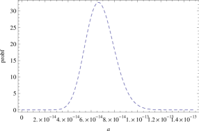
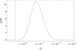
Figure 1: Probability density function for the scattering length (in $fm$) using 42 spiral galaxies radii and a dark matter particle mass of $10^{-6}\;eV$. The left panel shows the spin-0 case, and the right panel shows the spin-1 case.

The peak of the probability density function constructed from the Likelihood gives us the best fit for the parameter in investigation. We can see in figure (1) that the best value is around $10^{-14}\;fm$. Since we have overestimated the errors used in calculations, the width of this curve is also overestimated.

For the spin-1 case, we have to make some additional assumptions. We assume that the ferromagnetic phase scattering length $a_{2}^{f}$ and the polar phase scattering length $a_{2}^{p}$ have the same value, and that this does not differ from $a$ obtained for the spin-0 case. Using the previously calculated value as an input, we find the probability function for the scattering length $a_{0}^{p}$ as shown in the right panel of fig. (1). The best fit value for this quantity is around $10^{-13}\;fm$.

We also performed the same analysis using slightly higher values for the mass. Fig. (2) shows the case for a dark matter particle with a mass of the order of $10^{-5}\;eV$. The scattering length in this case is found to be $\sim 10^{-11}\;(10^{-10})\;fm$ for the spin-0 (spin-1) case.

Figure 2: Probability density function for the scattering length (in $fm$) using 42 spiral galaxies radii and a dark matter particle mass of $10^{-5}\;eV$. The left panel shows the spin-0 case, and the right panel shows the spin-1 case.

The case of a particle with a mass of the order $10^{-4}\;eV$ is shown in Fig. (3). The scattering length in this case is found to be $\sim 10^{-8}\;(10^{-7})\;fm$ for the spin-0 (spin-1) case.

Considering larger masses causes the scattering length to lie outside the upper bound referred to in section III.

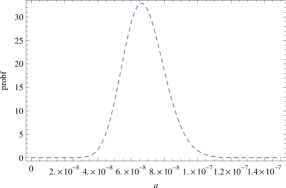
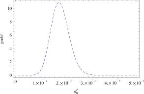
Figure 3: Probability density function for the scattering length (in $fm$) using 42 spiral galaxies radii and a dark matter particle mass of $10^{-4}\;eV$. The left panel shows the spin-0 case, and the right panel shows the spin-1 case.

Another sample, now containing 19 low surface brightness (LSB, dark matter dominated objects with $f_{DM}>0.9$) galaxies radii ranging from 1.2 to 19.6 $kpc$, obtained from lsb , have been analysed using the same method. The corresponding plots are shown in Figs. 4-6.

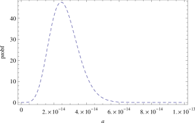
Figure 4: Probability density function for the scattering length (in $fm$) using 19 LSB galaxies radii and a dark matter particle mass of $10^{-6}\;eV$. The left panel shows the spin-0 case, and the right panel shows the spin-1 case.

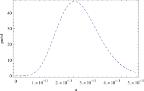
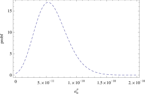
Figure 5: Probability density function for the scattering length (in $fm$) using 19 LSB galaxies radii and a dark matter particle mass of $10^{-5}\;eV$. The left panel shows the spin-0 case, and the right panel shows the spin-1 case.

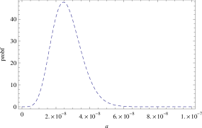
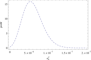
Figure 6: Probability density function for the scattering length (in $fm$) using 19 LSB galaxies radii and a dark matter particle mass of $10^{-4}\;eV$. The left panel shows the spin-0 case, and the right panel shows the spin-1 case.

The values of the scattering lengths obtained with the use of LSB galaxies do not differ from the previous results. A possible explanation for this behavior is that our expressions for the radius of the BEC fluid derived from Thomas-Fermi approximation depend only on the dark matter particle mass, and not on the astrophysical objects masses. Since the radii ranges are similar in both the galaxies sets we used, it is not surprising that the scattering lengths are also similar.

V Conclusions

In this work, we have been able to develop a theory for a spin-1 Bose-Einstein condensate composed of WISPs in terms of their scattering length and their masses. We could identify two phases of this condensation state, namely, a polar phase where the total angular momentum is zero, and a ferromagnetic phase where the total momentum is in the maximal projection.

Considering also spin-0 particles (related to axions or axion-like particles), it was possible to use this condensate to model dark matter halos in galaxies and obtain their radii in terms of the same parameters.

In order to constrain the values of scattering lengths and masses for the two possible condensate phases, we proceeded to a statistical analysis using a set of 42 dark matter dominated spiral galaxies and 19 LSB galaxies radii. Even though the set used presents a relativily small number of data, we have been able to limit the mass of the proposed dark matter particle to the range $10^{-6}-10^{-4}\;eV$ and to find the lower bound for the scattering length to be $10^{-14}\;fm$. We recall here that the upper bound for this quantity have been estimated to be at the value $10^{-6}\;fm$ by the use of colliding clusters data in har12 .

Using this method we were not able to determine the dark matter particle’s spin, because of the similarity between the spin-0 and ferromagnetic phase expressions for the galaxy radius as a function of the scattering length. Even considering the fluid to be composed of spin-1 particles, we were not able to distinguish the corresponding two phases by the use of this statistical analysis, since they are linked by the use of $a_{2}^{f}$ as an input for $a_{2}^{p}$in the construction of the probability functions . A more comprehensive analysis involving a significantly larger set of galaxy data may be necessary to establish this distinction beyond doubt. Nevertheless, one of the objectives of this paper is to show that this method can bring important information on the characteristics of the dark matter fluid.

The study of the condensate excitations and speed of sound could also allow the determination of the spin state of the fluid’s particles. These features can be related to the ocurrence of observable caustics and cusps in the galactic halo phase space sikivie2 and will be the subject of future work.

We would like to point out that one interesting feature of the present approach is the use of macroscopic quantities (e. g., astronomically determined galaxies’ radii) to gather information on microscopic parameters (particle masses and scattering lengths) related to quantum aspects of the nonrelativistic fluid. This correspondence is possible because we are treating a Bose-Einstein condensate. Another quantum fluid where this relation can be made is the degenerated Fermi fluid with half integer spin particles. This system will be treated in an upcoming work.

- (1) E. Komatsu et al., Astrophys. J., 192 18 (2011)
- (2) J. Beringer et al. (Particle Data Group), Phys. Rev. D 86 010001 (2012)
- (3) P. Arias et al., J. Cosmol. Astropart. Phys. 06 013 (2012)
- (4) A. E. Nelson and J. Scholtz, Phys. Rev. D 84, 103501 (2011)
- (5) R. D. Peccei, and H. R. Quinn, Phys. Rev. Lett. 38 1440 (1977); R. D. Peccei, and H. R. Quinn, Phys. Rev. D 16 1791 (1977)
- (6) J. Feng, Ann. Rev. Astron. Astrophys. 48 495 (2010)
- (7) S. -J. Sin, Phys. Rev. D 50, 3650 (1994); W. Hu, R. Barkana, and A. Gruzinov, Phys. Rev. Lett. 85, 1158 (2000); J. A. Vélez Pérez, Phys. Lett. B 671, 174 (2009)
- (8) P. Arias, J. Jaeckel, J. Redondo and A. Ringwald, Phys. Rev. D 82 15018 (2010)
- (9) O. Baker et al., Phys. Rev. D 85 035018 (2012)
- (10) P. Sikivie and Q. Yang, Phys. Rev. Lett. 103, 111301 (2009)
- (11) C. G. Böhmer and T. Harko, J. Cosmol. Astropart. Phys. 06, 025 (2007)
- (12) P.-H. Chavanis, Phys. Rev. D 84 043531 (2011)
- (13) P.-H. Chavanis and L. Delfini, Phys. Rev. D 84 043532 (2011)
- (14) V. Lora et al., J. Cosmol. Astropart. Phys. 02 011 (2012)
- (15) V. H. Robles and T. Matos, Mon. Not. Roy. Astron. Soc. 422, 282 (2012)
- (16) J. Stenger et al., Nature 396, 345 (1998)
- (17) C. J. Pethick and H. Smith, Bose-Einstein Condensation in Dilute Gases (2001) Cambridge-Press
- (18) S. W. Randall, M. Markevitch, D. Clowe, A. H. Gonzalez, and M. Bradac, Astrophys. J. 679, 1173 (2008)
- (19) T. Harko, and G. Mocanu, Phys. Rev. D 85, 084012 (2012)
- (20) T.-L. Ho, Phys. Rev. Lett. 81, 742 (1998)
- (21) A. Fetter and J. D. Walecka, Quantum Theory of Many-Particle System (1971) Dover
- (22) Y. Kawaguchi and M. Ueda, Phys. Rev. A 84, 053615 (2011)
- (23) M. W. Auger et al., Astrophys. J. 724, 511 (2010)
- (24) C. Trachternach et al., Astron. J. 136, 2720 (2008)
- (25) L. D. Duffy and P. Sikivie, Phys. Rev. D 78, 063508 (2008)