A GPU-Computing Approach to Solar Stokes Profile Inversion

Abstract

We present a new computational approach to the inversion of solar photospheric Stokes polarization profiles, under the Milne-Eddington model, for vector magnetography. Our code, named genesis (genetic stokes inversion strategy), employs multi-threaded parallel-processing techniques to harness the computing power of graphics processing units (gpus), along with algorithms designed to exploit the inherent parallelism of the Stokes inversion problem. Using a genetic algorithm (ga) engineered specifically for use with a gpu, we produce full-disc maps of the photospheric vector magnetic field from polarized spectral line observations recorded by the Synoptic Optical Long-term Investigations of the Sun (solis) Vector Spectromagnetograph (vsm) instrument. We show the advantages of pairing a population-parallel genetic algorithm with data-parallel gpu-computing techniques, and present an overview of the Stokes inversion problem, including a description of our adaptation to the gpu-computing paradigm. Full-disc vector magnetograms derived by this method are shown, using solis/vsm data observed on 2008 March 28 at 15:45 ut.

1. INTRODUCTION

Since Hale (1908) first inferred the presence of magnetic fields on the sun by observing the Zeeman-induced separation of the components of magnetically-sensitive spectral lines, the reliable determination of vector fields from spectral line observations has played a pivotal role in diagnosing solar magnetism. The Stokes vector, ${\bf I}_{\lambda}=[I_{\lambda},Q_{\lambda},U_{\lambda},V_{\lambda}]^{T}$, whose elements are linear combinations of measured polarization intensities at a wavelength $\lambda$, provide a convenient way to observe and characterize the effects of magnetic fields on the absorbing medium. Unno (1956) first described the Zeeman-induced attenuation of the Stokes vector by magnetic fields in the framework of the radiative transfer equations neglecting magneto-optical effects. The solution was later generalized to include magneto-optical (Faraday rotation) effects by Rachkovsky (1962).

Much information can be directly extracted from the observed Stokes vectors themselves; Rees & Semel (1979) developed a center-of-gravity technique for estimating the longitudinal component of the magnetic field from Stokes $I$ & $V$ observations, and Ronan et al. (1987) described an integral method for recovering the longitudinal and transverse fields from integrated Stokes linear and circular polarization profiles. Furthermore, several convenient weak-field calculation “recipes” can be found in Landi Degl’Innocenti (1994).

The unique specification of the magnetic and thermodynamic state of the solar photosphere solely from observations of the Stokes vector is classified as an “inverse” problem. These types of problems are often computationally complex and may be ill-conditioned. Conversely, the forward-modeling of the Stokes vector emergent from an assumed model atmosphere is trivial. This asymmetry can be exploited to interpret the observed Stokes vector within the framework of a magnetic model atmosphere, by tuning its configuration to minimize (in a least-squares sense) the model deviation from the observed Stokes vector. We collectively refer to all such solution procedures as “inversion methods.” Auer et al. (1977) developed a now traditional Stokes inversion method based on the Levenberg-Marquardt (l-m) algorithm (Levenberg, 1944; Marquardt, 1963), which was subsequently extended and improved upon by Skumanich & Lites (1987). This optimization approach performs a nonlinear least-squares fit of a Milne-Eddington model to the observations, returning the set of atmospheric parameters that describe the polarized spectral line. Ruiz Cobo & del Toro Iniesta (1992) extended the optimization method by creating an inversion code called sir (stokes inversion based on response functions), which performs the inversion of observed profiles while simultaneously inferring the stratification of the model parameters with optical depth.

More recently, artificial intelligence methods and pattern recognition approaches have been gaining ground in the computational methods of spectropolarimetric analysis. Carroll & Staude (2001) proposed a technique based on an artificial neural network (ann), whereby a large database of Stokes profiles (either synthetic or pre-inverted by some other means) is used to train the ann to recognize the functional relationship between the model parameters and the spectral lines in the training set. Once suitably trained, the network can generalize the relationship to other samples not explicitly included in the training set. Rees et al. (2000) developed a technique, based on the Principal Component Analysis (pca) formulated by Pearson (1901), to decompose a line profile into their so-called eigenprofiles. The eigenvalues associated with these eigenprofiles define a point in the model manifold, from which the associated model parameters can be calculated by interpolation over the training set. This method has been subsequently used on real observations by Socas-Navarro et al. (2001) and Eydenberg et al. (2005).

This paper introduces a new approach to the synthesis and inversion of spectral lines, based on graphics processing units (gpus), which can rapidly calculate full-disc vector magnetic fields at the photospheric level. The technique is based on the combination of a highly-parallel genetic algorithm with a computing architecture well suited to exploit the many levels of parallelism in the Stokes inversion problem. The remainder of this paper is organized as follows. Section 2 presents the observational data used in this work. Sections 3 and 4 outline our genetic algorithm optimization engine and gpu-programming techniques, respectively. Details of our implementation of Stokes inversion under the assumption of a Milne-Eddington atmosphere are given in Section 5. Results from the analysis presented in Section 6. Finally, we offer some outlooks on the future implementation of our method in the vector field data reduction pipeline for the Vector Spectromagnetograph (vsm), the scanning spectropolarimeter instrument package in operation as part of the Synoptic Optical Long-term Investigations of the Sun (solis) telescope, located at the National Solar Observatory atop Kitt Peak, AZ.

2. DATA & OBSERVATIONS

This work uses full-disc solis/vsm observations of the four Stokes $I$, $Q$, $U$, and $V$ spectra in a 3.45Å bandpass encompassing Fe i multiplet #816 near 6302Å (see Table 1). For this work, we utilize only the absorption line at $\lambda_{0}=6302.5017$Å, but note that our inversion code calculates the full Zeeman pattern of an input transition. Laboratory wavelengths for this multiplet and for two nearby terrestrial O₂ absorption features are taken from Pierce & Breckinridge (1973).

Table 1Line-formation parameters for Fe i multiplet #816.

Wavelength	Transition	$g_{\mathrm{eff}}$	$\chi_{e}$	$\log(gf)$
(Å)			(eV)
6301.5091	5P2–5D2	1.667	3.654	-0.718
6302.5017	5P1–5D0	2.500	3.686	-1.235

Figure 1 shows the solar disc as it was observed bysolis/vsm in the Stokes $I$ continuum (redward of 6302.5Å), on 2008 March 28 at 15:45 ut.

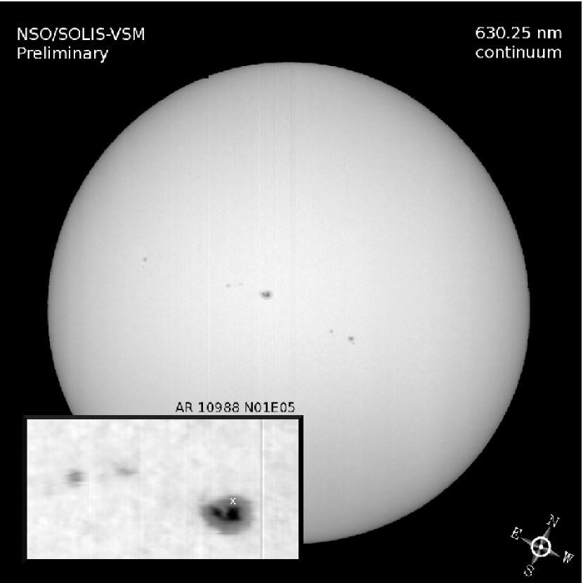
Figure 1.— Solar disc on 2008 March 28 15:45 ut as observed by the solis/vsm instrument in the 6302.5Å continuum. The compass points to heliographic solar north. The inset shows NOAA 10988 in more detail.

Figure 2 shows sample Stokes profiles taken from a penumbral region in NOAA 10988 (marked by the $\times$ symbol in Figure 1), close to disc-center. The somewhat low spatial resolution of solis/vsm pixels (1$\arcsec$.125 pixel^-1) smears the individual Zeeman components of the Fe i 6302.5Å line, preventing observation of fully resolved Zeeman lobes, even in sunspot umbrae where the splitting is largest.

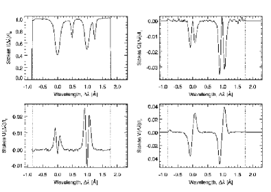
Figure 2.— Observed Stokes profiles (normalized by the local continuum) for a penumbral pixel (represented by the $\times$ symbol in the inset of Figure 1) belonging to NOAA 10988. solis/vsm spectral dispersion is $\Delta\lambda=27.1$ mÅ, and the wavelength scale is relative to the Fe i $\lambda$6301.5 line-core wavelength. The narrow, shallow lines are terrestrial O₂ absorption features, and are ignored in all analyses. The vertical lines denote the illumination edges of the CCD.

For the inversion of this dataset, our routines analyze only those pixels whose fractional polarization degree,

$$p=\frac{\sqrt{Q_{\mathrm{max}}^{2}+U_{\mathrm{max}}^{2}+V_{\mathrm{max}}^{2}}}{I_{c}},$$ (1)

exceeds a threshold set by the polarimetric noise, defined by

$$\sigma_{P}=P_{\mathrm{thresh}}\frac{\sqrt{\sigma_{Q}^{2}+\sigma_{U}^{2}+\sigma_{V}^{2}}}{I_{c}}$$ (2)

where $\sigma_{QUV}^{2}$ are the variances of the Stokes polarization profiles in a spectrally-quiet region away from the observed spectral lines, $I_{c}$ is the continuum intensity (determined in this same spectral window), and $P_{\mathrm{thresh}}$ is a proportionality factor. A value of $P_{\mathrm{thresh}}$ equal to unity will signal the inversion code to process all pixels with polarization degree strictly larger than the noise, while a value of $\sim 10$ typically provides good discrimination between active regions and surrounding quiet-sun, as observed by solis/vsm. While the spectral uncertainties will vary somewhat between scanlines and pixels, they are typically of the order of the vsm polarimetric accuracy ($\sim$ 0.1% of the continuum intensity). Pixels with polarization degree less than that given by equation 2 are inverted under the weak-field approximation; the longitudinal field strength is calculated from the separation between the $I{\pm}V$ line-cores, while the field orientation is calculated from Stokes $Q$, $U$, and $V$ maxima, as in Auer et al. (1977). To perform the inversion, we utilize a class of global optimization algorithms known as genetic algorithms.

3. A STANDARD GENETIC ALGORITHM

Genetic algorithms (gas) are a broad class of search and optimization algorithms which exploit computational analogues to the principles of evolutionary biology, first proposed by Darwin (1859). gas operate on (potential) solutions which are encoded into a binary representation. This requires distinction between the phenotypic expression (the parameters of the problem themselves) of the genotypic representation (the encoded parameters).

Genetic algorithms are receiving ever-increasing attention as powerful tools for search, optimization, and pattern recognition in fields as far-ranging as engineering design (Karr & Freeman, 1999), job-shop scheduling (Grefenstette, 1985), and stock market analysis (Mahfoud & Mani, 1996); Diver & Ireland (1997), McIntosh et al. (1998), and Ramirez & Fuentes (2002) have applied them to spectral analysis of nighttime astronomical observations; Charbonneau (1995) created the pikaia genetic algorithm and demonstrated its utility on several distinct problems of astrophysical importance, while Lagg et al. (2004) more recently applied the pikaia algorithm to the problem of diagnosing magnetic fields in the upper chromosphere with the He i triplet at 10830Å. They are quite robust, and often succeed where more traditional methods fail (e.g. multi-modal optimization).

The ga solution procedure relies on genetic operators which are repeatedly applied to a “parent” population of candidate solutions to produce a new “offspring” population of solutions, containing better solutions than those found in the previous population. The quantity which determines whether one solution is better than another is called the fitness, evaluated for each candidate solution via a fitness function. Here, the fitness function is a $\chi^{2}$-like merit score describing model deviations from observations. After some number of iterations of this process, the population will have converged to a small neighborhood around candidate solutions which have the best fitness scores. Although a comprehensive review of genetic algorithms and operators is well beyond the scope of this paper, we present here a simple overview of basic ga properties. An $N$-bit binary string is used to encode the $j^{th}$ model parameter,

$${\bf b}^{(j)}\equiv\left[b^{(j)}_{0}b^{(j)}_{1}b^{(j)}_{2}\cdots b^{(j)}_{N-1}\right],$$ (3)

where $b^{(j)}_{i}=\left[0,1\right]$, for each free parameter of the model. The convention adopted here is that bit $0$ is the most-significant bit, while bit $N-1$ is the least-significant bit. If the $j^{th}$ real-valued free parameter, ${\bf p}_{j}$, is constrained such that

$$u_{j}\leq{\bf p}_{j}\leq v_{j},$$ (4)

then each binary string can be decoded into a real floating-point value via the transformation:

$${\bf p}_{j}\equiv\mathcal{E}^{-1}({\bf b}^{(j)})=u_{j}+\frac{v_{j}-u_{j}}{2^{N}-1}\left[\sum_{k=0}^{N-1}{\bf b}^{(j)}_{N-k}\times 2^{k}\right].$$ (5)

The genetic algorithm population therefore consists of $N_{\mathrm{pop}}$ binary strings of the form:

$$\overbrace{\underbrace{1000010101001001}_{N\ {bits}}\cdots\underbrace{1010010100100101}_{N\ {bits}}}^{M{\times}N\ {bits}},$$ (6)

where $M$ represents the number of free parameters of the model. The following list elucidates the notation of Algorithm 1, which presents a pseudocode listing of the basic genetic algorithm functionality.

• ${\bf P}_{t}$ denotes the population of candidate solutions at generation $t$. Each (real-valued) candidate solution represents a single realization of a plane-parallel, Milne-Eddington m-e model of the line formation region. We seek the candidate whose forward-modeled Stokes vector shows minimum deviation from the observed profiles.

• ${\bf G}_{t}$ denotes the population of binary-encoded candidate solutions at generation $t$.

• ${\bf F}_{t}$ denotes the population fitness at generation $t$, and is generated by application of the evaluation operator, $\mathcal{F}$, to ${\bf P}_{t}$. Better candidate solutions will have smaller fitness values.

• The operator $\mathcal{S}$ represents sampling without replacement. The sampling is stochastically biased such that better candidate solutions are (probabilistically) more frequently selected from the population.

• The operator $\mathcal{E}$ represents the encoding of a candidate solution into its binary representation. An $N$-bit binary string gives a numerical resolution of $\Delta{p}_{i}=\left(v_{i}-u_{i}\right)/\left(2^{N}-1\right)$, if $u_{i}$ and $v_{i}$ are the lower and upper bounds, respectively, of the $i^{th}$ model parameter. The corresponding decoding operation (equation 5) is denoted by $\mathcal{E}^{-1}$.

• The operator $\mathcal{R}$ represents pair-wise recombination of the population. Two candidate solutions (selected by $\mathcal{S}$) swap segments of their binary representations to create the representations of two new offspring solutions.

• The operator $\mathcal{M}$ represents a probabilistic mutation for each member of the offspring population. Each bit on the binary string has a small probability of being flipped to its complementary bit. The mutation operator used in this work was designed to favor local exploration by mutating less-significant bits more frequently.

Algorithm 1 Pseudocode for a standard genetic algorithm.

  $t=0$

  Create ${\bf P}_{0}$

  Evaluate ${\bf F}_{0}\leftarrow\mathcal{F}[{\bf P}_{0}]$

  while  (not termination-condition)  do

     $t\leftarrow t+1$

     Select:    ${\bf P}_{t}\leftarrow\mathcal{S}[{\bf P}_{t-1},{\bf F}_{t-1}]$

     Encode:    ${\bf G}_{t}\leftarrow\mathcal{E}[{\bf P}_{t}]$

     Recombine:  ${\bf G}_{t}\leftarrow\mathcal{R}[{\bf G}_{t}]$

     Mutate:    ${\bf G}_{t}\leftarrow\mathcal{M}[{\bf G}_{t}]$

     Decode:    ${\bf P}_{t}\leftarrow\mathcal{E}^{-1}[{\bf G}_{t}]$

     Evaluate:  ${\bf F}_{t}\leftarrow\mathcal{F}[{\bf P}_{t}]$

  end while

We use gpu-computing techniques to offload data-parallel, compute- intensive calculations with high arithmetic intensity to a massively-parallel high-speed compute architecture. For this work, we employ an extension of the genetic algorithm inversion engine developed and described in Harker (2009) and a single nvidia Tesla C1060 gpu. We utilize nvidia’s Compute Unified Device Architecture (cuda) programming interface to handle data transfer and computations the gpu. The next section gives a brief introduction to structured parallel programming with cuda.

4. THE CUDA PROGRAMMING MODEL

The cuda programming interface consists of a minimal set of extensions to the standard C/C++ language which allow a properly-constructed data-parallel algorithm to execute among the thousands of concurrently running threads resident on the gpu. This is accomplished by a kernel function, which controls the computations and memory accesses to be performed at the thread granularity. The kernel function is callable from another user-defined function (the host function), which controls data transfers to/from the gpu and is responsible for launching the kernel execution.

A traditional criticism of the application of genetic algorithms to real-world problems is the fact that they tend to be slow, since they process a potentially large set of candidate solutions. The cuda programming interface allows nvidia gpus to execute such data-parallel algorithms, by organizing the computations into groups of concurrently-executing threads called blocks, while these blocks are themselves organized into groups of concurrently- executing grids. Mirroring this thread organization in the genetic algorithm population allows us to write a kernel function that dedicates each block to the calculations for a specific member of the population, while all threads in each block are dedicated to the per-wavelength calculations required by the spectral line synthesis and fitness function evaluation for each population member. The power of this approach is evident; in a serial genetic algorithm, the total number of wavelengths to synthesize (per generational iteration of Algorithm 1) is $N_{\lambda}N_{\mathrm{pop}}$, where $N_{\lambda}$ is the number of wavelengths spanning the spectral line, and $N_{\mathrm{pop}}$ is the size of the population. While this can only be done one wavelength at a time, one population member at a time for the serial algorithm, using a cuda-capable gpu allows all $N_{\lambda}N_{\mathrm{pop}}$ calculations to be done simultaneously, constrained only by the physical limitations of the gpu hardware itself (i.e., the maximum possible number of concurrently-executable threads and total onboard memory).

While a comprehensive review of the cuda architecture is outside the scope of this paper, we refer the interested reader to the cuda Programming Guide and Software Development Kit (sdk), currently available from http://www.nvidia.com/getcuda.

4.1. Thread & Memory Hierarchy

The cuda programming model requires an execution configuration, whereby the thread distribution is and organized into thread blocks, and similarly how individual thread blocks are organized into a grid. Figure 3 shows schematically how an example execution configuration is indexed, so that each thread can be uniquely identified in the grid.

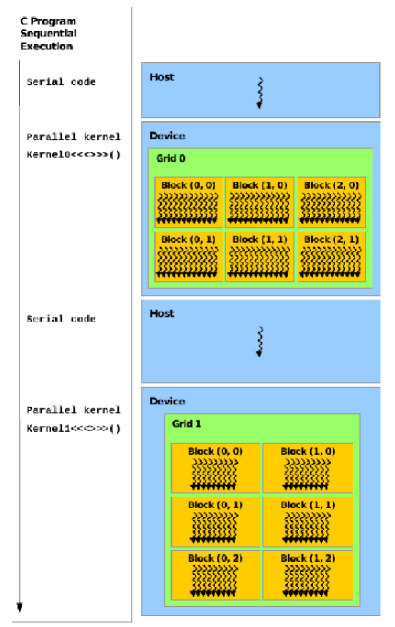
Figure 3.— cuda thread hierarchy ad heterogeneous computing paradigm. cuda kernel functions are interleaved with the host code, and multiple (potentially different) kernels may be launched from a host. The $<<<>>>$ syntax is one of the cuda extensions to the C language; it is used to specify the size and geometry of the execution configuration. Reproduced, with permission, from the cuda Programming Guide, courtesy of nvidia corporation. (NVIDIA Corp., 2011).

Threads from the same thread block may communicate with each other by utilizing shared memory (see below), although one must be careful to structure the program in such a way as to avoid memory access conflicts between threads. Global memory allows threads from different blocks to communicate with each other. Once the execution configuration is defined, the cuda kernel function is launched by invoking it with a special syntax, shown in Algorithm 2. Global memory for the input data and output result is allocated via cudaMalloc, and the data is copied from cpu memory to the allocated gpu memory with cudaMemcpy. The kernel function is invoked with nBlocks blocks of nThreads threads, and the desired results are copied back from device to host memory, again via cudaMemcpy. Please note, however, that an actual production-grade kernel invocation is considerably more involved than the toy example presented in Algorithm 2.

Algorithm 2 An example C-style cuda kernel invocation.

  cudaMalloc( (void**)&dResult, sizeof(hResult) );

  cudaMalloc( (void**)&dData, sizeof(hData) );

  cudaMemcpy( dData, hData, sizeof(hData),

              cudaMemcpyHostToDevice );

  MyKernel<<<nThreads, nBlocks>>>( dData, dResult );

  cudaMemcpy( dResult, hResult, sizeof(hResult),

              cudaMemcpyDeviceToHost );

4.2. Memory transfers between cpu and gpu

An important principle of gpu-computing is to minimize the amount of data that is copied between cpu memory and the global memory on the gpu. Bandwidth across the PCI-Express (pci-e) bus connecting cpu memory to gpu memory is much lower than the shared memory bandwidth, as can be seen in Table 2. The table shows the results of an initial bandwidth test performed on the gpu used in this work; these figures characterize our single realization of hardware components, and will vary depending on the exact system components and hardware specifications. The theoretical maximum bandwidth for the Tesla C1060 is 102 GB s^-1 (NVIDIA Corp., 2010), while we achieve $\approx 72$% of this theoretical limit in our hardware configuration.

Table 2Initial bandwidth tests for the nvidia Tesla C1060 used in this work.

Transfer Direction	Bandwidth
	(GB s-1)
cpu-to-gpu (global)	1.4634
gpu-to-cpu (global)	1.1840
gpu-to-gpu (shared)	73.3165

To maximize the efficiency of the data transfer to the gpu device, we modified our genetic algorithm by rephrasing the representation from the traditional binary arrays to unsigned short integer arrays. For example, consider a binary encoding of $M$ parameters with $N=16$ bits each. Instead of defining the binary genotype string as char gene[M*N], with gene[i] = 0 or 1 (see equation (6)), the genotype is defined as unsigned short gene[M], since each unsigned short is internally represented by 16 bits. The former encoding technique requires $8\times M\times N$ bits of storage, while the latter requires only $M\times N$ bits, representing a savings in storage space (and transfer times) of a factor of 8. Furthermore, the traditional encoding technique is incredibly wasteful, since only the least-significant bit of each $8$-bit char is needed to encode a 0 or 1, meaning only 1/8 of the data transferred to the gpu memory would actually be useful. In contrast, our modified binary genotype encodes the same amount of useful information, but occupies a fraction of the space in memory.

Transferring the binary encoded parameters to the gpu allows the threads to use the high-speed shared memory to decode the unsigned short integers to the real floating-point values needed for the model synthesis on the gpu, so this is always a net gain in performance over decoding the parameters serially and transferring the real floating-point values to the gpu.

This modified binary genotype also allows our genetic operators to use the bit-shifting and bit-masking techniques of Iuspa & Scaramuzzino (2001) to operate directly on the internal binary representation of the unsigned short integers. These bit-manipulation techniques yield faster genetic operators than would be used for the traditional binary representation, which typically involve several nested loops for analysis of each bit in the binary array.

We have presented the computational aspects of our gpu code in this section, so we now turn to the implementational details of our inversion and synthesis routines to be run on the gpu.

5. IMPLEMENTATION OF STOKES INVERSION

The polarized radiative transfer equations (prte) describe the modification of the Stokes vector of a beam as it propagates, in the direction $s$, through some medium. Formally, it is given here as

$$\mu\frac{d{\bf I}_{\lambda}}{ds}={\bf K}_{\lambda}\left({\bf I}_{\lambda}-{\bf S}_{\lambda}\right),$$ (7)

where $\mu$ is the cosine of the heliocentric angle, and ${\bf K}_{\lambda}$ and ${\bf S}_{\lambda}$ are the propagation matrix and source function vector, respectively.

If we model both continuum and line absorption processes, then

$${\bf K}_{\lambda}={\bf 1}+\eta_{0}{\bf\Phi}_{\lambda},$$ (8)

where $\eta_{0}$ is the ratio of line-to-continuum absorption coefficients, and the matrix ${\bf\Phi}_{\lambda}$ includes absorption and magneto-optical effects, parameterized by the magnetic and thermodynamic properties of the model atmosphere. Expressions for these matrix elements may be found in (e.g.) Landi Degl’Innocenti & Landolfi (2004) and references therein. These matrix elements are functions of the Voigt and Faraday-Voigt line profiles, calculated to high accuracy via the rational function approximation of Hui et al. (1978). This formulation is extremely well-suited to evaluation on a gpu, due to its high arithmetic intensity (ratio of math operations to memory accesses).

The source function vector describes the ratio of emission to absorption in the beam, and includes both continuum and line contributions, so that

$${\bf S}_{\lambda} = S_{c}{\bf\hat{e}}+\eta_{0}S_{l}{\bf\Phi}_{\lambda}{\bf\hat{e}},$$ (9)

$${\bf\hat{e}} = \left(1,0,0,0\right)^{T},$$ (10)

where $S_{c}$ is the continuum source function and $S_{l}$ is the line source function. Assuming local thermodynamic equilibrium reduces both continuum and line source function to the Planck function at the local temperature, $B_{\lambda}(T)$. Adopting a Milne-Eddington (m-e) relation for the source function variation as a linear function of optical depth,

$$S_{c}=S_{l}=B_{\lambda}(T)=S_{0}+S_{1}\tau=S_{0}(1+\beta_{0}\tau),$$ (11)

where $\beta_{0}=S_{1}/S_{0}$ represents the inverse of the characteristic length scale over which the source function changes appreciably, the prte admits an analytical solution for the model Stokes profiles, ${\bf I}_{\lambda}^{M}$, given here as

$$\frac{{\bf I}_{\lambda}^{M}}{I_{c}} = \left[\left(1-\beta\right){\bf 1}+\beta\left({\bf 1}+\eta_{0}{\bf\Phi}_{\lambda}\right)^{-1}\right]{\bf\hat{e}}$$ (12)

$$\beta = \frac{\mu\beta_{0}}{1+\mu\beta_{0}},$$ (13)

where ${\bf 1}$ is a $4\times 4$ identity matrix and $I_{c}$ denotes the observed local continuum intensity. This m-e solution is characterized by magnetic and thermodynamic parameters assumed to be constant with depth through the line-formation region, here collectively represented by the model vector of free parameters, ${\bf p}$. Since we do not consider gradients with respect to optical depth of any parameter except the source function, the m-e atmosphere represents a kind of integrated behavor of the true parameters over the height of line-formation (Orozco Suárez & Del Toro Iniesta, 2007). Formally, the $k^{th}$ candidate solution in the genetic algorithm represents a single model vector

$${\bf p}_{k}\equiv[B,\psi,\chi,\lambda_{0},a_{\mathrm{dc}},\Delta\lambda_{D},\eta_{0},S_{0},\beta_{0}]^{T},$$ (14)

where $B$ is the magnetic field strength, $\psi$ is the inclination of the field with respect to the observer’s line of sight, $\chi$ is the azimuthal angle of the field, $\lambda_{0}$ is the line-center wavelength of the spectral line, $a_{dc}$ is the atomic damping constant of the spectral line, $\Delta\lambda_{D}$ is the Doppler line-width, $\eta_{0}$ is the line-to-continuum opacity ratio, and $S_{0}$ and $\beta_{0}$ are the linear source function coefficients such that the continuum intensity is given by the Eddington approximation as

$$I_{c}=S_{0}+\mu{S_{1}}=S_{0}\left(1+\beta_{0}\mu\right),$$ (15)

To maintain generalizability in the inversion code, the full Zeeman pattern of the spectral line is calculated at the start of inversion. This is done only once, so the overhead incurred is negligible, considering the flexibility gained. The particular spectral line to be synthesized is configurable by the user, and the code contains all the necessary generalizations of the m-e solutions to allow it to function with arbitrary photospheric spectral lines. The fitness function to be minimized by the genetic algorithm is the following $\chi^{2}$-like merit function, which quantifies the fit of the Stokes vector (${\bf I}^{M}$) generated by the model ${\bf p}_{k}$ (with $\nu=4N_{\lambda}-M$ degrees of freedom) to the observations (${\bf I}^{O}$), given here explicitly as

$$\chi^{2}({\bf p}_{k})=\frac{1}{\nu}\sum_{i}\sum_{j=1}^{N_{\lambda}}w^{2}_{ij}\left[{\bf I}^{O}_{i}(\lambda_{j})-{\bf I}^{M}_{i}(\lambda_{j};{\bf p}_{k})\right]^{2},$$ (16)

where $i=I,Q,U,V$. The quantities $w_{ij}$ are weighting factors, traditionally used to adjust the contribution of different wavelengths to the total deviation across the spectral line, and are discussed further in Section 5.4. Here, the $j$ index is dropped from the weights; they are taken as constant over the spectral line, but distinct for each of the four Stokes profiles. Using this form of the merit function allows the calculation of uncertainties (over the $\chi^{2}$ hypersurface) in the recovered model parameters by straightforward techniques, once the genetic algorithm has converged.

It is an important principle of optimization to work in the smallest possible parameter space; reducing the dimensionality of the model vector will increase the speed of the inversion and enhance the stability of the algorithm, since there are fewer (potentially degenerate) parameters to simultaneously determine. The next section describes some of the techniques used in our approach to reduce the dimension of the parameter space and therefore enhance the efficiency of the genetic search.

5.1. Reduction of the model manifold

Although the line-center wavelength can be a free parameter of the fit, genesis instead directly uses the observed line-center wavelength as measured from the core of the Stokes $I$ profile. After calibrating the observed wavelength scale by measuring the separation of the two terrestrial O₂ absorption lines near 6302Å, a center-of-symmetry approach,

$$\lambda_{\mathrm{sym}}\equiv\underset{\lambda_{i}}{\mathrm{{\bf argmin}}}\ S(\lambda_{i})=\displaystyle\sum_{j}|I(\lambda_{i+j})-I(\lambda_{i-j})|$$ (17)

is used to determine a rough estimate of the line-center wavelength. This estimate is refined by bracketing $\lambda_{sym}$ with a wavelength triplet and calculating the minimum of its uniquely-fit polynomial.

The m-e model atmosphere specifies a source function linear in optical depth, characterized by its value at the ${\tau}=0$ photospheric surface ($S_{0}$) and its inverse characteristic length scale ($\beta_{0}$). Inspection of the Unno-Rachkovsky solutions reveals a simple normalization scheme that eliminates the dependence on $S_{0}$, as was adopted in Auer et al. (1977). Here, we define a modified Stokes vector,

$${\bf I}^{M}_{\lambda}\leftarrow I_{c}{\bf\hat{e}}-{\bf I}_{\lambda}^{M},$$ (18)

which consists of the Stokes $I$ line depression and Stokes $Q$, $U$, and $V$ profiles. Note we choose to leave $\beta_{0}$ (which influences the amplitude of the synthesized Stokes profiles) as a free parameter of the fit.

5.2. Limited spatial resolution & scattered light

To account for limited spatial resolution, a new free parameter is introduced; the magnetic fill-fraction $\alpha$ represents the fractional pixel area occupied by the magnetic field. The remainder of the pixel area ($1-\alpha$) is assumed to be field-free. The Stokes vector then becomes a linear superposition of the magnetic and non-magnetic profiles, weighted by $\alpha$,

$${\bf I}^{M}_{\lambda}\leftarrow\alpha{\bf I}^{M}_{\lambda}+(1-\alpha)I^{\mathrm{nm}}_{\lambda}{\bf\hat{e}}.$$ (19)

The non-magnetic profile is assumed to be a quiet-sun Stokes $I$ profile from the local surroundings. Using a locally-averaged quiet-sun profile would require breaking one of the most advantageous properties of the algorithm, namely that each scanline/pixel can be inverted independently of the data from neighboring scanlines/pixels. Furthermore, this approach requires a tremendous amount of disk I/O, and can be quite slow. To maintain a totally independent scanline inversion, we have taken a different approach; the center-to-limb variation (CLV) of the quiet-sun Stokes $I$ profile has been measured (Harvey, 2010, private communication) and parameterized as a pure Voigt function characterized by its amplitude, full-width at half-maximum (FWHM) and atomic damping parameter. Gaussian and Lorentzian components of the profile can be derived from the FWHM. A 3^rd-order polynomial is fit (as a function of heliocentric $\mu$) to the CLV of each of these parameters. The resulting polynomial fits are used within the inversion to calculate the appropriate values of the quiet-sun parameters as a function of disc position for each pixel. The non-magnetic profile is then synthesized from these parameters, centered on the observed Stokes $I$ line-center wavelength.

We account for scattered light at the $\sim$5% level by first correcting the measured continuum. The baseline of the observed Stokes $I$ profile is increased, and subsequently renormalized to the corrected continuum, following Gray (2005).

5.3. Thermodynamic parameters

It is well known that there exists some level of degeneracy between the magnetic and thermodynamic parameters, with respect to their influence on the model profile line-shapes. Figure 11.1 of del Toro Iniesta (2003) shows an explicit example of this effect; it is not always clear whether one combined magnetic and thermodynamic configuration leads to a better fit to the observations than another, even if the configurations are noticeably different (Borrero et al., 2011). The convention typically adopted by inversion practitioners is that the thermodynamic model parameters are of less importance to the final quality of the fit than the magnetic parameters. Skumanich & Lites (1987) suggested that in order to find a robust fit, some of the thermodynamic parameters must be fixed prior to the inversion, and Borrero et al. (2011) investigated the effects of holding the atomic damping at a constant value during their inversions. They found negligible differences between the recovered vector magnetic fields. It is not clear, however, that this procedure is generally acceptable for observations with much higher spectral resolution than in Borrero et al. (2011). We have decided not to hold fixed any of the thermodynamic parameters, and have implemented a “pre-fitting” initialization in which we fit a non-magnetic Stokes $I$ profile to the observed Stokes $I$ profile, using a simple Levenberg-Marquardt algorithm. This returns values for the atomic damping parameter, $a_{\mathrm{dc}}$, Doppler width $\Delta\lambda_{D}$, line-to-continuum opacity ratio, $\eta_{0}$, and source function parameter, $\beta_{0}$. Assuming a non-magnetic model for a (potentially) Zeeman-broadened profile will, of course, lead to errors in the derived thermodynamic variables. However, these values are utilized only to constrain the parameter space to sensible ranges within which the ga can search.

5.4. Weighting scheme

Since the Stokes $I$ profile will always have much larger signal strengths than the polarization profiles, deviations between the observed and synthesized Stokes $I$ profiles will dominate the $\chi^{2}$ value, essentially causing the algorithm to fit the model atmosphere solely to the Stokes $I$ intensity profile. To mitigate this effect, we equalize the importance of all four Stokes profiles by using an “inverse-max” weighting scheme to ensure that all deviations contribute roughly equally to the calculated $\chi^{2}$. The weighting scheme is given here explicitly as:

$$w_{I} = \left(I_{c}-I_{0}^{\mathrm{obs}}\right)^{-1}$$ (20)

$$w_{Q} = \left(\max\ |Q^{\mathrm{obs}}_{\lambda}|\right)^{-1}$$ (21)

$$w_{U} = \left(\max\ |U^{\mathrm{obs}}_{\lambda}|\right)^{-1}$$ (22)

$$w_{V} = \left(\max\ |V^{\mathrm{obs}}_{\lambda}|\right)^{-1},$$ (23)

where $I_{0}^{\mathrm{obs}}$ is the observed line-core intensity.

5.5. Model manifold boundaries

The genetic inversion will be most efficient in a parameter space that has the smallest physically-realistic domain for each parameter. By seeding the initial population of the genetic algorithm with some specific heuristic knowledge of the problem at hand, we can both ensure that we start with at least a few high-quality solutions, and suitably restrict the domain of the searchable parameter space. Both scenarios will accelerate the convergence and improve the final accuracy of the solutions.

Here, the initial population includes representations of magnetic field vectors generated from the weak-field approximations in Auer et al. (1977), as well as from a functional relationship between the field geometry and integrated measures of the Stokes polarization profiles found in Ronan et al. (1987). The longitudinal field strength estimated from the center-of-gravity approach by Rees & Semel (1979) is also seeded into the initial population. In the case of full-disc inversions, where every on-disc pixel is inverted, the trivial non-magnetic solution is seeded into the population as well.

The field inclination domain is naturally restricted to a single polarity, $\psi\in[0,90]^{\circ}$ or $[90,180]^{\circ}$, initialized to be in agreement with the order of the blue- and red-lobes of the observed Stokes $V$ profile. The seed fields are checked to ensure that they are consistent with this polarity.

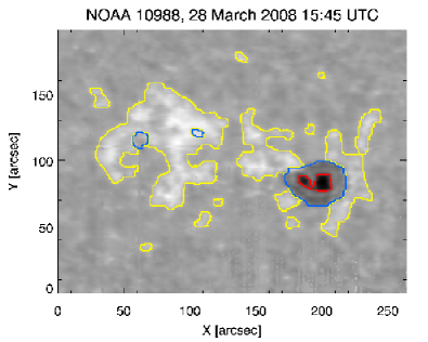
Figure 4.— Line morphology classification for NOAA 10988. The image depicts Stokes $I$ line-core intensity, overlaid with red, blue, and yellow contours demarcating umbral, penumbral, and plage regions, respectively.

Additionally, we use empirical knowledge derived specifically from solis/vsm data to discriminate between different magnetic structures observed on the disc. Spatial pixels are labeled as likely belonging to the structures seen in Figure 4, based on their observed continuum and line-core intensities relative to the average quiet-sun profile. Following Hestroffer & Magnan (1998), we apply a simple correction for limb-darkening to flatten the observed intensity profile in pixels far from disc-center, before a label is assigned. The details of this empirical classification scheme (and the subsequent compartmentalization of the $B$-$\alpha$ subspace) are given in Table 3.

Table 3Active region structure discrimination parameters.

discriminator	Umbra	Penumbra	Plage
$I_{c}/I_{c}^{qs}$	$<$ 0.65	[0.65-0.90]	$>$ 0.90
$I_{0}/I_{0}^{qs}$	$<$ 0.69	$>$ 0.69	$>$ 0.85
$B\ [G]$	[1000-3500]	[0-2500]	[0-1500]
$\alpha$	[0.25-1]	[0.25-1]	[0-0.5]

5.6. Population initialization

As described in Section 3, the genetic algorithm works by continually evolving good solutions out of a population of candidate solutions, represented by the reduced model vectors

$${\bf p}_{k}\equiv[B,\psi,\chi,a_{\mathrm{dc}},\Delta\lambda_{D},\eta_{0},\beta_{0},\alpha]^{T},$$ (24)

with the number of free parameters, $M=8$. Hardware limitations dictate the maximum size of the population; the Tesla C1060 gpu contains 30 multiprocessors, each of which is composed of 8 stream processors. Therefore, the total number of thread blocks (candidate solutions) which can be simultaneously processed is $N_{\mathrm{pop}}=30\times 8=240$.

It is traditional to initialize the genetic algorithm with a random (but bounded) population to ensure enough diversity for the genetic operators to produce meaningful evolution. However, we instead generate the initial population (of non-seeded candidate solutions) by repeatedly sampling from a Sobol sequence generated via the Bratley & Fox (1988) algorithm. An $M$-dimensional Sobol sequence is a quasi-random sequence that is maximally self-avoiding; the points in the sequence tend to (roughly) evenly distribute themselves throughout the $M$-dimensional hypercube $[0,1]^{M}$. This property gives robust, even coverage of the parameter space without placing the initial population on a regularized grid, which would completely inhibit the search action of the recombination operator ($\mathcal{R}$). In addition, this approach eliminates chance clustering in the initial population, thereby avoiding the processing of redundant candidate solutions. The final benefit of using quasi-random initialization lies in the efficiency of population restarts; when the population has converged to some self-monitored degree, all but the best individual(s) are re-initialized. Generating new candidates according to a quasi-random schedule guarantees that we will be refreshing the “gene pool” in the most efficient way, by using the self-avoidance property to automatically ignore previously-sampled regions of the parameter space. We exploit this property to address any issues related to premature/false convergence; every $N_{\mathrm{samp}}$ iterations of the genetic algorithm, we discard the worst half of the population (“dead solutions”) and reinitialize them according to the Sobol mechanism described above. In practice, for a maximum number of generations $N_{\mathrm{gen}}$ over which to evolve, we note that $N_{\mathrm{samp}}\approx N_{\mathrm{gen}}/4$ provides a good balance between deep genetic search and the introduction of new genetic material. We allow the population to evolve for $N_{\mathrm{gen}}=100$ generations.

6. RESULTS & DISCUSSION

Proceeding along each scanline and performing the genesis inversion on the corresponding spectra for each pixel builds a map of the model parameters over the full-disc. Figure 5 shows the magnetic field strength, inclination, azimuthal angle, and fill-fraction over the full-disc as inferred by the genesis inversion. The inset shows NOAA 10988.

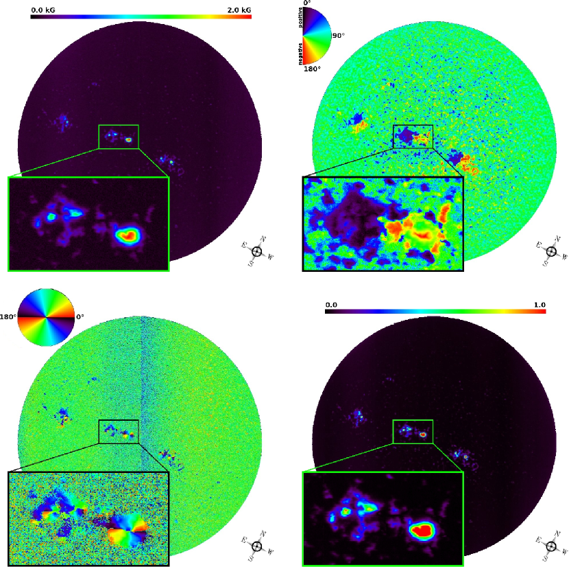
Figure 5.— (top left): field strength, (top right): field inclination, (bottom left): field azimuth, (bottom right): fill-fraction. The vertical stripe down the center of the azimuthal angle image is an artifact of the dual Rockwell camera system in solis/vsm, and do not appear in newer Sarnoff camera data. The compass points to solar north.

The $0^{\circ}$ reference direction for the azimuthal angle is along the horizontal axis of the image. The field has not been resolved of the $\pi$-ambiguity inherent in all Stokes inversion techniques, hence the antisymmetric color wheel Nevertheless, the radial structure of penumbral fields is well-determined. The fill-fraction displays the expected behavior of values $\approx$ 1 for the umbral and penumbral regions, with a decline to values $\leq$ 0.5 for surrounding plage regions.

The statistical spread of the final population provides a convenient means to generate initial estimates of the uncertainties associated with the fitted model parameters. Measuring the spread around the identified optimum gives population uncertainties, from which we estimate the gradient of the $\chi^{2}$ manifold:

$$\left[\nabla\chi^{2}\left({\bf p}^{\mathrm{opt}}\right)\right]_{j}\approx\frac{\chi^{2}\left({\bf p}^{\mathrm{opt}}\right)-\chi^{2}\left({\bf p}_{i}\right)}{\left[\Delta{\bf p}\right]_{j}},$$ (25)

where ${\bf p}_{i}$ is selected from the best of the final population, chosen such that we avoid numerical difficulties in the calculation of the finite differences (i.e. ratio of two very small numbers). Using this estimate, we bootstrap the derivatives to higher accuracy by Richardson extrapolation to zero stepsize within Neville’s algorithm (see, e.g., Press et al., 1988). The Hessian matrix, ${\bf H}$, is thus calculated as the Jacobian of the resulting gradient vector and the variance of the $i^{th}$ model parameter is given by Sanchez Almeida (1997):

$$\sigma_{\mathrm{p}_{i}}^{2}=\left[{\bf H}^{-1}\right]_{ii}\frac{\chi^{2}({\bf p}^{\mathrm{opt}})}{M}.$$ (26)

This evaluation requires a (potentially) large number of fitness function calls, but is only done once per pixel, so the small overhead incurred is outweighed by the benefit of having an accurate error estimate for the model parameters.

Table 4Distribution of uncertainties in Fe i $\lambda 6302.5$ magnetic parameters, broken down by structure.

Structure	$\Delta_{B}\pm\sigma_{\Delta_{B}}$	$\Delta_{\gamma}\pm\sigma_{\Delta_{\gamma}}$	$\Delta_{\chi}\pm\sigma_{\Delta_{\chi}}$	$\Delta_{\alpha}\pm\sigma_{\Delta_{\alpha}}$
	(G)	(∘)	(∘)	($\times 10^{-3}$)
Umbra	1.3$\pm$2.9	0.45$\pm$0.69	0.73$\pm$0.89	2.4$\pm$5.9
Penumbra	2.4$\pm$4.5	0.62$\pm$0.80	0.73$\pm$0.91	2.5$\pm$5.4
Plage	1.2$\pm$2.7	0.65$\pm$0.79	0.84$\pm$0.96	2.1$\pm$3.6

Table 4 presents an estimation of the uncertainties in the fitted model parameters determined in this manner. The uncertainties are broken down according to the structure discrimination method in Section 5.5. For each structure, we calculate the average uncertainty, $\Delta_{i}$, and corresponding standard deviation, $\sigma_{\Delta_{i}}$. The table shows the quantity $\Delta_{i}\pm\sigma_{\Delta_{i}}$, so that $\Delta_{i}+3\sigma_{\Delta_{i}}$ represents an upper limit to the model parameter uncertainties in 99.73% of the pixels belonging to each active region structure. For example, 99.73% of umbral pixels have uncertainties in field strength of 10 G or less. These quantities are not meant to represent the uncertainties in any particular pixel or structure, but instead characterize the overall distribution of uncertainties derived from the inversion. It should be noted, however, that these uncertainties are derived solely from the topology of the $\chi^{2}$ hypersurface, and do not include systematic errors resulting from the assumptions and/or limitations of the Milne-Eddington model, which is sometimes not a suitably accurate description of the real solar atmosphere.

Table 5Timing profiles for genesis inversions of Fe i $\lambda\lambda$6301.5,6302.5

mode	$\Delta T_{\mathrm{run}}$		$\Delta T_{\mathrm{eval}}$
	(min)		(min)
	6301.5Å	6302.5Å	6301.5Å	6302.5Å
serial	187.83$\pm$0.69	84.56$\pm$0.26	147.54$\pm$0.68	55.53$\pm$0.17
gpu-acc.	36.40$\pm$0.15	32.82$\pm$0.36	4.43$\pm$0.01	2.34$\pm$0.01

Table 5 shows a speed comparison between the serial and gpu-accelerated versions of the genesis inversion code, for both iron lines, averaged over 50 independent runs. The total evaluation time ($\Delta T_{\mathrm{eval}}$) is the time spent synthesizing the model spectra and evaluating the various contributions to equation 16. For the serial code, the evaluation time consumes a strong majority (65.7% and 78.5% for Fe i $\lambda$6302.5 and Fe i $\lambda$6301.5, respectively) of the total algorithm runtime, $\Delta T_{\mathrm{run}}$. Use of the gpu as a co-processor has reduced the total evaluation time to only 7.1% and 12.1%, respectively, of the gpu-accelerated total runtime. The total runtime is quite stable for both the serial and gpu-accelerated versions of the code. The table shows $1\sigma$ standard deviations, which demonstrate that the serial and gpu- accelerated versions can vary in their total runtimes by up to a minute. The gpu-accelerated evaluation time further shows why the gpu chip architecture is so amenable to parallel computations. The variation in the average time spent interacting with the gpu is less than a second; this stability is precisely due to the many-cored nature of the gpu, which uses a very efficient thread scheduler to keep the cores of each multiprocessor optimally busy.

Overall, the gpu-accelerated Fe i $\lambda$6302.5 inversion is a factor of 2.6 times faster than the serial version, with an increase to a factor of 5.2 for the Fe i $\lambda$6301.5 non-normal triplet. The total synthesis and evaluation time shows just how powerful the cuda programming paradigm can be, performing the computations 23.7 and 33.3 times faster than the serial versions of the code can manage. Since the non-normal triplet Fe i $\lambda$6301.5 has four contributions (from levels with equal $\Delta{M_{J}}$) to each of the three Zeeman components, a greater proportion of work is done on the gpu. This highlights another principle of gpu computing; the more work you assign to the gpu, the more efficiently it can perform it.

7. CONCLUSIONS

We have described a novel computational approach to the inference of photospheric vector magnetic fields from observations of the Stokes polarization profiles. Our new inversion code, named genesis, is capable of quickly producing full-disc spatial maps of the magnetic structure of the solar photosphere observed by the solis/vsm instrument located atop Kitt Peak at the National Solar Observatory, in a fraction of the time required by a similar serial technique. The inversion code is capable of recovering magnetic fields with uncertainties on the order of 0.5%, with errors in the field orientation of a few degrees. Fill-fractions are recovered with uncertainties on the order of 2%. Currently, the code is only capable of inverting a single line at a time, though we plan to investigate the extension to the simultaneous inversion of both lines of the Fe i $\lambda$6302 multiplet.

We have shown the technique to be amenable to the reduction and analysis of large volumes of spectropolarimetric data. To this end, we are currently investigating the the assimilation of the gpu hardware and specialized cuda-based algorithms into the solis/vsm vector field pipeline. Our long-term goals for this work are to provide near real-time vector magnetic fields to the scientific community. Increasing the cadence of solis/vsm vector data products will also allow us to support and complement observations taken by the Solar Dynamics Observatory (sdo) Helioseismic and Magnetic Imager (hmi), which produces full-disc vector magnetograms at $4096\times 4096$ resolution with a cadence of approximately 12 minutes.

The gpu programming paradigm is highly scalable; a compiled cuda application can execute on any cuda-capable device, subject to hardware limitations. The thread scheduler will automatically allocate the appropriate number of thread blocks to the stream processors. Coupled with the Message Passing Interface (mpi) to parallelize over scanlines (i.e. independent scanlines are inverted independently, utilizing their own distinct gpu), this could lead to incredibly fast (i.e. near-realtime or realtime) full-disc inversions with a modest number of cpu-gpu pairs. Improvements in gpu hardware are steadily advancing; the Fermi architecture is the recent successor to the Tesla architecture, offering up to 512 cuda cores, larger-capacity memory banks, and increased floating-point performance. With the next-generation Kepler architecture on the horizon, the prospects for accelerated solar data processing are indeed promising. Finally, as gpu computing matures, we expect to extend this approach to better hardware, with a cautious eye toward spectropolarimetric analyses of data recorded by the upcoming Advanced Technology Solar Telescope (atst). The volume of data expected from this next-generation observatory will greatly exceed that of the current generation, requiring new and faster techniques to properly handle and reduce the observations in a timely manner. We feel the integration of gpu-accelerated data-reduction techniques will be key for the analysis of such large datasets, and may make available important (near) real-time information on the photospheric vector magnetic field to the space-weather forecasting community.

References

- Auer et al. (1977) Auer, L. H., House, L. L., & Heasley, J. N. 1977, Sol. Phys., 55, 47
- Borrero et al. (2011) Borrero, J. M., Tomczyk, S., Kubo, M., et al. 2011, Sol. Phys., 273, 267
- Bratley & Fox (1988) Bratley, P., & Fox, B. L. 1988, ACM Trans. Math. Softw., 14, 88
- Carroll & Staude (2001) Carroll, T. A., & Staude, J. 2001, A&A, 378, 316
- Charbonneau (1995) Charbonneau, P. 1995, ApJS, 101, 309
- Darwin (1859) Darwin, C. 1859, On the Origin of Species by Means of Natural Selection (London, U.K., W. Clowes and Sons)
- del Toro Iniesta (2003) del Toro Iniesta, J. C. 2003, Introduction to Spectropolarimetry (Cambridge, UK: Cambridge University Press, April 2003.)
- Diver & Ireland (1997) Diver, D. A., & Ireland, D. G. 1997, Nuclear Instruments and Methods in Physics Research A, 399, 414
- Eydenberg et al. (2005) Eydenberg, M. S., Balasubramaniam, K. S., & López Ariste, A. 2005, ApJ, 619, 1167
- Gray (2005) Gray, D. F. 2005, The Observation And Analysis Of Stellar Photospheres (Cambridge University Press)
- Grefenstette (1985) Grefenstette, J. J., ed. 1985, Proceedings of the 1st International Conference on Genetic Algorithms, Pittsburgh, PA, USA, July 1985 (Lawrence Erlbaum Associates)
- Hale (1908) Hale, G. E. 1908, ApJ, 28, 315
- Harker (2009) Harker, B. J. 2009, PhD thesis, Utah State University
- Hestroffer & Magnan (1998) Hestroffer, D., & Magnan, C. 1998, A&A, 333, 338
- Hui et al. (1978) Hui, A., Armstrong, B., & Wray, A. 1978, Journal of Quantitative Spectroscopy and Radiative Transfer, 19, 509
- Iuspa & Scaramuzzino (2001) Iuspa, L., & Scaramuzzino, F. 2001, Soft Computing - A Fusion of Foundations, Methodologies and Applications, 5, 58, 10.1007/s005000000066
- Karr & Freeman (1999) Karr, C. L., & Freeman, L. M. 1999, Industrial Applications of Genetic Algorithms, CRC Press International Series On Computational Intelligence (CRC Press)
- Lagg et al. (2004) Lagg, A., Woch, J., Krupp, N., & Solanki, S. K. 2004, A&A, 414, 1109
- Landi Degl’Innocenti (1994) Landi Degl’Innocenti, E. 1994, in Solar Surface Magnetism, ed. R. J. Rutten & C. J. Schrijver, 29
- Landi Degl’Innocenti & Landolfi (2004) Landi Degl’Innocenti, E., & Landolfi, M., eds. 2004, Astrophysics and Space Science Library, Vol. 307, Polarization in Spectral Lines
- Levenberg (1944) Levenberg, K. 1944, Quarterly of Applied Mathematics, 2, 164
- Mahfoud & Mani (1996) Mahfoud, S., & Mani, G. 1996, Applied Artificial Intelligence, 10, 543
- Marquardt (1963) Marquardt, D. W. 1963, SIAM Journal on Applied Mathematics, 11, 431
- McIntosh et al. (1998) McIntosh, S. W., Diver, D. A., Judge, P. G., et al. 1998, A&AS, 132, 145
- NVIDIA Corp. (2010) NVIDIA Corp. 2010, Tesla C1060 Computing Processor Board: Board Specifications (NVIDIA Corp.)
- NVIDIA Corp. (2011) —. 2011, NVIDIA CUDA C Programming Guide (NVIDIA Corp.)
- Orozco Suárez & Del Toro Iniesta (2007) Orozco Suárez, D., & Del Toro Iniesta, J. C. 2007, A&A, 462, 1137
- Pearson (1901) Pearson, K. 1901, Philosophical Magazine, 2(6), 559
- Pierce & Breckinridge (1973) Pierce, A. K., & Breckinridge, J. B. 1973, The Kitt Peak Table of Photographic Solar Spectrum Wavelengths, Contribution (Kitt Peak National Observatory) (Kitt Peak National Observatory)
- Press et al. (1988) Press, W. H., Teukolsky, S. A., Flannery, B. P., & Vetterling, W. T. 1988, Numerical Recipes in C (Cambridge University Press)
- Rachkovsky (1962) Rachkovsky, D. N. 1962, Izv. Krymsk. Astrofiz. Obs., 27, 148
- Ramirez & Fuentes (2002) Ramirez, J., & Fuentes, O. 2002, Experimental Astronomy, 14, 129, 10.1023/B:EXPA.0000009933.44289.e4
- Rees et al. (2000) Rees, D. E., López Ariste, A., Thatcher, J., & Semel, M. 2000, A&A, 355, 759
- Rees & Semel (1979) Rees, D. E., & Semel, M. D. 1979, A&A, 74, 1
- Ronan et al. (1987) Ronan, R. S., Mickey, D. L., & Orrall, F. Q. 1987, Sol. Phys., 113, 353
- Ruiz Cobo & del Toro Iniesta (1992) Ruiz Cobo, B., & del Toro Iniesta, J. C. 1992, ApJ, 398, 375
- Sanchez Almeida (1997) Sanchez Almeida, J. 1997, ApJ, 491, 993
- Skumanich & Lites (1987) Skumanich, A., & Lites, B. W. 1987, ApJ, 322, 473
- Socas-Navarro et al. (2001) Socas-Navarro, H., López Ariste, A., & Lites, B. W. 2001, ApJ, 553, 949
- Unno (1956) Unno, W. 1956, PASJ, 8, 108