Casimir force of expulsion

Abstract

The possibility in principle is shown that the noncompensated Casimir force can exist in nanosized open metal cavities. The force shows up as time-constant expulsion of open cavities toward their least opening. The optimal parameters of the angles of the opening, of “generating lines” of cavities and their lengths are found at which the expulsive force is maximal. The theory is created for trapezoid configurations, in particular for parallel mirrors which experience both the transverse Casimir pressure and longitudinal compression at zero general expulsive force.

To find such geometrical configurations of nanosized bodies, at which the Casimir repulsion of the bodies, often associated with levitation and buoyancy effects, can take place, is an urgent task (see, for example,  Leonhardt:2007 ; Levin:2010 ; Rahi:2011 . However, the levitation is possible only at limited distances from the surface of bodies-partners. Much more promising and important is the search of geometrical shapes which can have Casimir noncompensated force causing the effect of continuous expulsion of a configuration in a certain direction independent of the proximity to the surfaces of bodies-partners. The objective of the present work is to demonstrate such possibility.

When the volume of a quantum field is bounded by material boundaries, there can be not only Casimir attraction force Casimir:1948 but the effects of neutral “buoyancy” of curved surfaces Jaffe:2005 and other interesting phenomena as well (see, for example,  Bordag:2001 ; Rodriguez:2011 ). The Casimir classical result for two planes is obtained by assuming that they are infinite and, correspondingly, all the other components of the energy-momentum tensor (EMT) of the electromagnetic field are compensated except those that are normal to the surface. Naturally, in the case with objects having finite sizes the application of the classical Casimir result cannot reflect all possible occurrences of zero electromagnetic-field oscillations. The calculations of Casimir forces for particular configurations are rather complicated Brown:1969 . Therefore, light variants of approximated calculations are used taking into account only the existence of EMT components normal to a surface. Such approximation is the one of Deryagin Derjaguin:1956 for short-range Van der Waals forces, within the frames of which the Casimir forces between microspheres and a surface (see, for example, Bordag:2006 ) and some other similar configurations are calculated. The discrepancies between the magnitudes of forces calculated with the use of the proximity force approximation (PFA) and true magnitudes of Casimir forces can be much more than 0.1% Gies:2006 since there is an essential difference in the nature and long-range action of Casimir and Van der Waals forces. At present new methods for the calculation of forces for different configurations are being looked for (see, for example,  Bordag:2009 ; Pavlovsky:2011 ; Jaffe:2004 ; Graham:2010 ; Rahi:2012 ; Zaheer:2010 ). The method based on classical geometrical optics can be mentioned as one of the most promising  Jaffe:2004 ; Scardicchio:2005 . However, none of the existing approaches allows to demonstrate the existence of Casimir expulsive forces in any configurations. It is due to the fact that normally problems are focused upon the interaction of parts of the configuration of a body or bodies-partners.

Let us consider a configuration with a trapezoid cavity which will serve as an example for the demonstration of the possibility in principle that the Casimir expulsive forces can exist. Cavity should be understood as an open thin-walled metal shell with one or several outlets. The inner and outer surfaces of the cavity should have the properties of perfect mirrors. The cavity should entirely be immerged into a material medium or be a part of the medium with the parameters of dielectric permeability being different from those of physical vacuum. In Cartesian coordinates the configuration looks like two thin metal plates with the surface width $L$ (oriented along the $z$-axis) and length $R$, which are situated at a distance $a$ from one another; the angle $2\varphi$ of the opening of the generating lines of cavities between the plates can be varied (by the same value $\varphi$ simultaneously for both wings of the trapezoid cavity) as it is shown in  Fig.11.

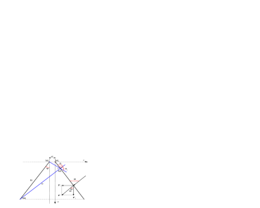
Figure 1: Schematic view of the configuration of a symmetric trapezoid cavity with the length $R$ of the wing surface, a particular case of which is parallel planes, i.e. $\varphi=0$, and a triangle at $a=0$. The section of the cavity shown in the Cartesian coordinates in the plane ($x,z$) has the width $L$ in the $y$ direction normal to the plane of the figure. The blue straight lines designate virtual rays with the length $b$ coming from the point $\mbox{M}_{1}$ at limit angles $\Theta_{1}$ and $\Theta_{2}$ onto the right cavity surface ending at the ends of the opposite cavity wing at the points $\mbox{M}_{2}$ and $\mbox{M}_{3}$, respectively.

Further, let us use the following formalism. Let us take the so-called tensor of Casimir stress for the electromagnetic field between two parallel plates separated by the distance $a$, which is determined in 4D space-time coordinates $(tc,\hat{x},\hat{y},\hat{z})$ Brown:1969 ; Fulling:2007 in the form

$$T^{{}^{\mu\nu}}=\frac{E_{c}}{a}\mbox{diag}(1,-1,-1,3),$$ (1)

where the Casimir energy per unit of area is $E_{c}=-\frac{\hbar c\pi^{2}}{720{\kern 1.0pt}a^{3}}.$ Here, $\hbar=h/2\pi$ is the reduced Planck constant, $c$ is the velocity of light. We use only the component $P_{c}=T^{33}$ of the stress tensor for each point $r$ on the cavity surface. However, let us note that the coordinates $(\hat{x},\hat{y},\hat{z})$ in 4D space are not the same as the coordinates on our drawing plane $(x,y,z)$.

For solving the problem let us assume that virtual photons have the properties of rays and are strictly specularly reflected from the perfectly conducting metal walls both inside and outside the cavities. As a first approximation, we assume that this property of rays is characteristic of all lengths of waves of the electromagnetic spectrum. For each ray incident at the angle $\Theta$ on the cavity surface from the outside there is a strictly opposite corresponding ray coming from the inside. The action of the pulses of the above rays results in the presence of the local (at the point $r$) specific Casimir force which is noncompensated for each direction $\Theta$ on the outer surface of the cavity. It means that the Casimir pressure of each individual ray incident on the point $r$ at any of the angles $\Theta$ will correspond to the value

$$P_{c}(a,\varphi,\Theta,r)=-\frac{\hbar c\pi^{2}}{240\,b^{4}},$$ (2)

where $b=f(r,a,\varphi,\Theta).$ The force action of each ray in our coordinates $(x,y,z)$ is decomposed into components directed along $x-$ and $z-$axes. The component directed against the $z$-axis is associated with the specific force (pressure) acting upon the cavity surface and its sign conforms to the sign of the Casimir pressure in formula (2). The component directed along the $x$-axis (its sign should be +) is associated with the specific force of expulsion of the entire configuration (or the force of sliding of one cavity wing relative to the other when one plate is fixed and the other is not).

The material medium both inside and outside metal cavities, in principle, can have dielectric permeability $\varepsilon$ different from that of vacuum. This fact like many others (temperature Brown:1969 , etc.) can be taken into account; however, further we shall consider an ideal situation.

The operator of turning of the right wing of the configuration through the angle $\varphi$ and of each ray at any local point $r$ (with the angles $\Theta$ between the rays and the cavity surface as in Fig.1) can be written in the form

$$\phi^{i}=\left[{{\begin{array}[]{*{20}c}{\cos(\Theta-\varphi)\hfill}\\ {\sin(\Theta-\varphi)\hfill}\\ \end{array}}}\right].$$ (3)

The local stress tensor at the point $r$ in our coordinates $(x,z)$ can be expressed as

$$P_{ik}=P_{c}\left[{{\begin{array}[]{*{20}c}{-1\hfill}&0\hfill\\ 0\hfill&1\hfill\\ \end{array}}}\right].$$ (4)

Then the integral quantities for Casimir pressures along the $x-$ and $z$-axes at the point $r$ at all possible angles $\Theta$ are

$$P_{k}(r)=\int\limits_{\Theta_{1}}^{\Theta_{2}}P_{ik}\phi^{i}d\Theta.$$ (5)

The entire Casimir force of compression (at $P_{z}=P_{22})$ acting thus upon one of the plates along the $z$-axis in our coordinates $(x,y,z)$ can be expressed as follows

$$F_{z}=\int\limits_{0}^{L}{dy}\int\limits_{0}^{R}{dr}\int\limits_{\Theta_{1}}^{\Theta_{2}}P_{c}(\varphi,\Theta,r)\sin(\Theta-\varphi)d\Theta.$$ (6)

The entire Casimir force of expulsion (at $P_{x}=P_{11})$ along the $x$-axis is

$$F_{x}=-\int\limits_{0}^{L}{dy}\int\limits_{0}^{R}{dr}\int\limits_{\Theta_{1}}^{\Theta_{2}}P_{c}(\varphi,\Theta,r)\cos(\Theta-\varphi)d\Theta.$$ (7)

Here for the given geometry the limit angles are $\Theta_{1}=f(r,a,\varphi)\;$and $\Theta_{2}=f(r,a,\varphi)$. Let us find these angles using geometric notion of directing vectors corresponding to the rays for limit angles $\Theta_{1},\;\Theta_{2}$ and to the ”generatrix” of the right wing of the cavity on the schematic view of the trapezoid configuration (Fig.1). Let us designate the point data on the trapezoid cavity scheme: $M_{0}(x_{0},z_{0})$, $M_{1}(x_{1},z_{1})$, $M_{2}(x_{2},z_{2})$ and $M_{3}(x_{3},z_{3})$. Then, the vector $\overrightarrow{M_{0}M}_{1}=(x_{1}-x_{0};z_{1}-z_{0})$ is chosen as a directing vector of the straight line of the “generatrix” of the cavity right wing. $\overrightarrow{M_{1}M}_{2}=(x_{2}-x_{1};z_{2}-z_{1})$ is chosen as a directing vector of the ray $b$. Let us choose $\overrightarrow{M_{1}M}_{3}=(x_{3}-x_{1};z_{3}-z_{1})$ as a vector of the ray between the extreme upper point of the left wing $M_{3}(x_{3},z_{3})$ and the point $M_{1}(x_{1},z_{1})$. The corresponding coordinates can be written in the form: $x_{0}=0$; $z_{0}=0$; $x_{1}=r\cos\varphi$; $z_{1}=r\sin\varphi$; $x_{2}=R\cos\varphi$; $z_{2}=-R\sin\varphi-a$; $x_{3}=0$; $z_{3}=-a$. The cosines of the angles between the guiding lines are defined as $\cos\Theta_{1}=\frac{\overrightarrow{M_{0}M}_{1}\cdot\overrightarrow{M_{1}M}_{2}}{\left\|{\overrightarrow{M_{0}M}_{1}}\right\|\cdot\left\|{\overrightarrow{M_{1}M}_{2}}\right\|}$ and $\cos{\Theta_{2}}=\frac{{{{\overrightarrow{{M_{0}}M}}_{1}}\cdot{{\overrightarrow{{M_{1}}M}}_{3}}}}{{\left\|{{{\overrightarrow{{M_{0}}M}}_{1}}}\right\|\cdot\left\|{{{\overrightarrow{{M_{1}}M}}_{3}}}\right\|}}.$ Thus, the expressions for $\Theta_{1},\;\Theta_{2}$ and $b$ have the forms

$\Theta_{1}=\mbox{arccos}\left({-\frac{r+a\sin\varphi-R\cos 2\varphi}{\sqrt{\left({a+R\sin\varphi+r\sin\varphi}\right)^{2}+\left({r\cos\varphi-R\cos\varphi}\right)^{2}}}}\right),$ $\Theta_{2}=\mbox{arccos}\left({-\frac{r+a\sin\varphi}{\sqrt{a^{2}+r^{2}+2ra\sin\varphi}}}\right),$ $b=\frac{\sin(2\varphi-\Theta_{2})(a+r\sin\varphi)}{\sin(\Theta-2\varphi)\sin(\varphi-\Theta_{2})}.$

Let us consider the nature of the non-compensation of the forces along the $x$-axis. The integration (5) by all the angles $\Theta$ for local specific forces of compression in the $z$ direction gives

$$\begin{gathered}{P_{z}}(r)=-\frac{{\hbar c{\pi^{2}}}}{{{{240}}{s^{4}}}}\int\limits_{{\Theta_{1}}}^{{\Theta_{2}}}{}\sin{(\Theta-2\varphi)^{4}}\sin(\Theta-\varphi)d\Theta,\end{gathered}$$ (8)

where $s=\frac{\sin(2\varphi-\Theta_{2})(a+r\sin\varphi)}{\sin(\varphi-\Theta_{2})}.$ By integrating (5) by all the angles $\Theta$ for local specific forces of expulsion in the $x$ direction we obtain

$$\begin{gathered}{P_{x}}(r)=\frac{{\hbar c{\pi^{2}}}}{{{{240}}{s^{4}}}}\int\limits_{{\Theta_{1}}}^{{\Theta_{2}}}{}\sin{(\Theta-2\varphi)^{4}}\cos(\Theta-\varphi)d\Theta.\end{gathered}$$ (9)

We should note that when the actions at the angles $\Theta$ are taken into account, for parallel plates ($\varphi=0$) at $R\to\infty$ the pressure $P_{z}(R)$ is larger than that calculated by Casimir in ${16}/{15}$ by a factor of $\mathop{\lim}\limits_{\varphi\to 0,\;R\to\infty}P_{z}(R)\to-\frac{\hbar c\pi^{2}}{240\,s^{4}}\frac{16}{15}$ according to expression (8).

In this case, for the same limits, specific forces of expulsion $P_{x}(r)$ tend to zero as it should hold in the given configuration $\mathop{\lim}\limits_{\varphi\to 0,\;\,R\to\infty}P_{x}(R)\to 0.$ However, the solution of (9) in the limits from $\Theta_{1}=0$ to $\Theta_{2}=\pi/2$ and, separately, from $\Theta_{1}=\pi/2$ to $\Theta_{2}=\pi$ gives

$$P_{x}(\varphi\to 0,R\to\infty)=\frac{\hbar c\pi^{2}}{240s^{4}}\left\{{\begin{array}[]{l}-\frac{1}{5};\;0\leq\Theta\leq\frac{\pi}{2}\\ +\frac{1}{5};\frac{\pi}{2}\leq\Theta\leq\pi.\\ \end{array}}\right.$$ (10)

It means that the configuration of two parallel plates shrinks both along the $z$-axis and the $x$-axis with the specific force of the order of 1/5 of the classical Casimir specific force and 16/75 of that determined by formula (8).

Thus, here we have a basic scheme of the calculation of the Casimir forces of pressure and expulsion in geometric approximation. Perhaps, it is possible to construct the theory of Casimir forces of expulsion based on first principles. However, the solutions of these and even more traditional problems encounter essential difficulties. Known attempts to calculate Casimir pressure dependences in wedged geometries with angle $2\varphi$ between the surfaces of the cavity lead to the results which are far from being real Deutsch:1979 ; Dowker:1978 .

The use of formulae (4-9) allows to reveal the following character of Casimir specific forces $P_{z}(r)$ and $P_{x}(r)$ along the $x$-axis for two parallel plates ($\varphi=0$) of the same length $R$ with the distance between them $a=4\times 10^{-7}$  m (see Fig. 2). The same character of the dependences will take place at rescaling the dimensional parameters of a configuration to any small values but, naturally, within the frames of physically reasonable limits restricted by sizes of atoms.

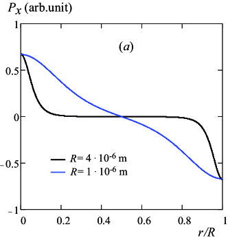
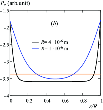
Figure 2: Specific local Casimir forces of expulsion ($a$) and pressure ($b$) along the $x$-axis at $\varphi=0$. The red line ($b$) shows the classical level of the Casimir pressure.

In Fig. 2$b$ it can be seen that at $R/a\geqslant 1$ the specific force $P_{z}(r)$ on the boundaries is always half of that in the centre of the configuration. The smaller are the configuration sizes, the more uniform are the compression forces. In addition, it can be seen that in the configuration there are forces $P_{x}(r)$ compressing the ends of the parallel plates toward their centre (Fig. 2$a$). The specific force of compression is $16/75$ of the specific force of pressure $P_{z}(r)$ on the plates. In this case, the smaller is the length $R$, the larger part of the cavity wing is subjected to the action of such forces. However, along the $x$-axis, the integral Casimir forces $P_{x}(r)$ compensate one another.

An essentially different situation can be observed when we start changing the angle $\varphi$ which is half of the angle between the cavity surfaces. It can be seen in Fig. 3 that at all the angles $\varphi\neq 0$ there is a noncompensated force $P_{x}(r)$ pushing the figure along the $x$-axis both in the positive and negative directions. The result of the action of the noncompensated force will be called Casimir expulsion.

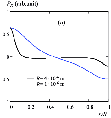
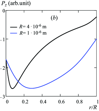
Figure 3: Specific local Casimir forces of expulsion and compression along the $x$-axis at the angles $\varphi=1\mathring{}$ ($a,b$).

Along the $x$-axis locally near the narrower section of the trapezoid cavity the force pushing the cavity in the $x$ direction prevails at small angles. However, at the further growth of the angle $\varphi$ in the proximity of the narrow section of the cavity the forces pushing it in the opposite direction to the $x$-axis are growing.

Having ultimately integrated $P_{x}(r)$ and $P_{z}(r)$ by $x$ we will find the entire Casimir force $F_{x}$ and $F_{z}$ acting upon one wing of the cavity. Let us study its dependence on the wing length $R$. The corresponding results are displayed in Fig. 4.

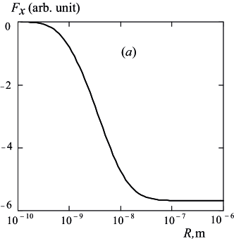
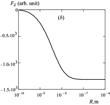
Figure 4: Entire Casimir force of expulsion ($a$) and compression ($b$) of the cavity wing at $\varphi=1\mathring{}$ depending on the wing length $R$ and width $L$ = 1   m.

As seen from Fig.4$a$, the total force of expulsion is always oppositely directed to the $x$-axis. The force appears as time-constant expulsion of the open trapezoid cavity in the direction of its least opening (i.e. in the direction of smaller section).

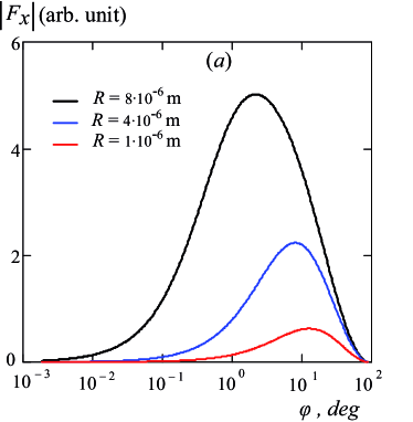
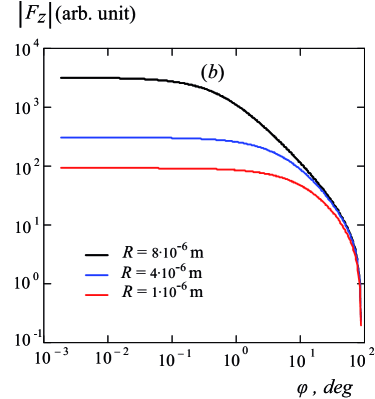
Figure 5: Absolute values of the Casimir forces of expulsion ($a$) and compression ($b$) for different lengths $R$ depending on the angle $\varphi$.

Fig. 5$a$ show the dependence of total forces of expulsion and compression on the angle $\varphi$. It is seen that for any length of the surfaces of the cavity there is an expulsion maximum depending on the angle $\varphi$, and the larger is the length $R$, the smaller is the angle.

The existence of noncompensated forces of expulsion is possible for any other open metal cavities. However, trapezoid cavities have the most diverse and effective properties for study and application.

Thus, here the possibility in principle is shown that noncompensated Casimir force of expulsion can exist in configurations in the form of open (perfectly conducting) metal nanosized cavities. The force is capable of creating constant directed thrust which does not require the presence of bodies-partners. The force essentially differs from forces of repulsion capable of creating only effects such as levitation over bodies-partners. It is shown that for a trapezoid configuration, forces of expulsion have optimums both for sizes and angles between cavity surfaces at which their manifestation is maximal. A particular case of trapezoid cavities is parallel mirrors. It is shown here that among many other things parallel mirrors experience both transverse and longitudinal compression due to the oppositely-directed expulsion forces acting upon the ends of the mirrors. However for strictly parallel mirrors all the forces of expulsion are compensated in all directions.

- (1) U. Leonhardt, New J. Phys. 9, 254 (2007).
- (2) M. Levin et al., Phys. Rev. Lett. 105, 090403 (2010).
- (3) S. J. Rahi, S. Zaheer, Phys. Rev. Lett. 104, 070405 (2010).
- (4) H. B. G. Casimir, Kon. Ned. Akad. Wetensch. Proc. 51, 793 (1948).
- (5) R. L. Jaffe, A. Scardicchio, J. High Energy Phys. 6, (2005) arXiv:hep-th/0501171v2.
- (6) G. L. Klimchitskaya, U. Mohideen, and V. M. Mostepanenko, Rev. Mod. Phys. 81, 1827 (2009).
- (7) A. W. Rodriguez, F. Capasso & S. G. Johnson, Nature Photonics 5, 211 (2011).
- (8) L. S. Brown, G. J, Maclay, Phys. Rev. 184, 1272 (1969).
- (9) B. V. Derjaguin, I. I. Abrikosova, E. M. Lifshitz, Q. Rev. Chem. Soc. 10, 295 (1956).
- (10) M. Bordag, Phys. Rev. D 73, 125018 (2006).
- (11) H. Gies, K. Klingmuller, Phys. Rev. Lett. 96, 220401 (2006).
- (12) M. Bordag, V. Nikolaev, Phys. Rev. D 81, 065011 (2010).
- (13) O. Pavlovsky, M. Ulybyshev, J. Mod. Phys. A. 25, 2457 (2011) arXiv:0911.2635v1.
- (14) R. L. Jaffe, A. Scardicchio, Phys. Rev. Lett. 92, 070402 (2004).
- (15) N. Graham, A. Shpunt, T. Emig, et al., Phys. Rev. D 81, 061701 (2010).
- (16) S. J. Rahi, T. Emig, R. L. Jaffe, Lecture Notes in Physics, 834, 129 (2011) arXiv:1007.4355v1.
- (17) S. Zaheer, S. J. Rahi, T. Emig, R. L. Jaffe, Phys. Rev. A 82, 052507 (2010).
- (18) A. Scardicchio, R. L. Jaffe, Nucl. Phys. B 704, 552 (2005).
- (19) S. A. Fulling et al, Phys. Rev. D 76, 025004 (2007).
- (20) D. Deutsch, P. Candelas, Phys. Rev. D. 20, 3063 (1979).
- (21) J. S. Dowker, G. Kennedy, J. Phys. A. Math. Gen. 11, 895 (1978).