Tracing Cold H I Gas in Nearby, Low-Mass Galaxies

Abstract

We analyze line-of-sight atomic hydrogen (H I) line profiles of 31 nearby, low-mass galaxies selected from the Very Large Array - ACS Nearby Galaxy Survey Treasury (VLA-ANGST) and The H I Nearby Galaxy Survey (THINGS) to trace regions containing cold (T $\lesssim$ 1400 K) H I from observations with a uniform linear scale of 200 pc beam^-1. Our galaxy sample spans four orders of magnitude in total H I mass and nine magnitudes in M_B. We fit single and multiple component functions to each spectrum to isolate the cold, neutral medium given by a low dispersion ($<$6 km s^-1) component of the spectrum. Most H I spectra are adequately fit by a single Gaussian with a dispersion of 8-12 km s^-1. Cold H I is found in 23 of 27 ($\sim$85%) galaxies after a reduction of the sample size due to quality control cuts. The cold H I contributes $\sim$20% of the total line-of-sight flux when found with warm H I. Spectra best fit by a single Gaussian, but dominated by cold H I emission (i.e., have velocity dispersions $<$6 km s^-1) are found primarily beyond the optical radius of the host galaxy. The cold H I is typically found in localized regions and is generally not coincident with the very highest surface density peaks of the global H I distribution (which are usually areas of recent star formation). We find a lower limit for the mass fraction of cold-to-total H I gas of only a few percent in each galaxy.

1 Introduction

Dwarf irregular (dIrr) galaxies in the nearby universe are laboratories for studying the most fundamental properties of gas evolution and star formation. Large, multi-wavelength studies of these systems are only just beginning. However, recent, high resolution surveys of large, spiral galaxies in the ultraviolet (e.g., NGS - Gil de Paz et al. 2007), optical (e.g., NFGS - Jansen 2000; ANGST - Dalcanton et al. 2009), infrared (e.g., SINGS - Kennicutt et al. 2003), and radio (e.g., THINGS - Walter et al. 2008; HERACLES - Leroy et al. 2009) have given us insight into where and when stars form in a galaxy. They have also provided clues to the gas conditions surrounding sites of current star formation (Leroy et al. 2008; Bigiel et al. 2008). The conclusion is that stars form in regions rich in cold, dense, molecular material (Kennicutt, 1998; Kennicutt & Evans, 2012). These studies mainly focus on high metallicity systems, however. How these results translate to low metallicity environments has not been fully explored, mainly due to the fact the most commonly observed tracer of molecular material, CO, is notoriously difficult to observe at low metallicity (e.g., Taylor et al. 1998; Barone et al. 2000; Leroy et al. 2005; Schruba et al. 2012).

Nearby dIrr galaxies offer the opportunity to study the star formation process in low metallicity systems at high spatial resolution. Studies of the star formation rates in dIrr galaxies defined from UV, 24$\mu$m, and/or H$\alpha$ emission (e.g., Leroy et al. 2008; Bigiel et al. 2008; Roychowdhury et al. 2009) have found a non-linear correlation with the local atomic hydrogen (H I) distributions. However, the dependence of star formation on molecular gas content is apparent in the large spiral galaxies observed in Leroy et al. (2008) and Bigiel et al. (2008). The star formation rate surface density is shown to correlate linearly with the molecular gas surface density in these galaxies. These results can be understood if one assumes that efficient star formation requires molecular hydrogen (e.g., Krumholz et al. 2009 and references therein).

Based on theoretical studies, the very character of the interstellar medium (ISM) is likely to change at low metallicity (e.g., Spaans & Norman 1997). Glover & Mac Low (2011) modeled the so called X-factor which measures the relationship between amount of detected CO emission and the abundance of molecular hydrogen. They found that the amount of CO drops substantially at low metallicities, consistent with prior predictions (e.g., Maloney & Black 1988). This deficit of CO at low metallicities is supported by observations showing relatively low or no detections of CO emission in nearby dIrr galaxies (e.g., Taylor et al. 1998; Barone et al. 2000; Leroy et al. 2005; Schruba et al. 2012). Consequently, this lack of metals also results in lower amounts of polycyclic aromatic hydrocarbon (PAH) emission (e.g., Engelbracht et al. 2005; Jackson et al. 2006). The PAHs are important to the formation of the cold ISM since they are critical in the shielding of UV and soft X-ray photons.

The long standing problem of studying the molecular component in the low metallicity dwarfs continues. We expect dIrr galaxies to contain molecular hydrogen since they are forming stars. However, since direct observations of the molecular gas responsible for forming stars in large samples of dIrr galaxies via CO are currently not feasible, we must find a different tracer of star-forming gas.

One intriguing idea is to find the immediate precursors of the molecular gas. The assembly of star forming molecular clouds is generally believed to require cold H I (e.g., Wolfire et al. 2003; Krumholz et al. 2009). In our galaxy, cold H I clouds have been observed to surround and even intermix with molecular clouds (e.g., Krčo & Goldsmith 2010) through studies of H I narrow self absorption (HINSA; Li & Goldsmith 2003). One promising technique to find cold H I gas was pioneered by Young & Lo (1996, 1997) in a sample of nearby, star forming dIrr galaxies. These authors used high angular and spectral resolution H I data of two nearby dIrr galaxies to decompose line-of-sight spectra into narrow and broad Gaussian components. The narrow-lined gas ($\sigma$ $\sim$ 4.5 km s^-1) was found only in specific regions within the H I disk while the broad-lined gas ($\sigma$ $\sim$ 10 km s^-1) was found along every line-of-sight observed. The narrow Gaussian component was attributed to cold (T$\lesssim$1000 K) H I gas while the broad lined gas was assumed to be warm, neutral hydrogen (T$\gtrsim$5000 K). Young et al. (2003) studied three more dIrr galaxies, finding that they, too, contained evidence for cold H I gas. Other authors have used this technique to discover cold H I in a small number of other galaxies. de Blok & Walter (2006) investigated the H I distribution in NGC 6822 and also found regions rich with cold H I gas. Recent work by Begum et al. (2006) found evidence of cold H I gas in six dIrr galaxies from the Faint Irregular Galaxies GMRT Survey (FIGGS; Begum et al. 2008). To date, cold H I in emission has been discovered in 10 nearby dIrr galaxies.

Within the limited data available, different measurements of the cold H I do appear to give comparable results. Two galaxies, DDO 210 and GR8, from the sample of Young et al. (2003) overlapped with that of Begum et al. (2006). Young et al. (2003) used the Very Large Array (VLA) at a linear scale of $\sim$200 pc beam^-1 with a velocity resolution of 1.3 km s^-1 while Begum et al. (2006) used the Giant Metrewave Radio Telescope (GMRT) at a linear resolution of $\sim$300 pc beam^-1 with a velocity resolution of 1.65 km s^-1. Despite the use of different facilities and different spatial/spectral resolutions, both studies find similar results for both the spatial distributions and velocity dispersions of the narrow component. This agreement between the two studies suggests that the measurement of cold H I is generally robust, and not extremely sensitive to the exact observing parameters.

The technique of identifying a cold neutral medium has also been used in nearby, high metallicity spiral galaxies. Braun (1997) isolated cold H I gas using relatively low spectral resolution (6 km s^-1) imaging from the VLA for 11 of the closest spiral galaxies. He combined spectra from discrete radial bins and found that these combined spectra all had a narrow Gaussian core (FWHM $\lesssim$ 6 km s^-1) superposed onto broad (FWHM $\sim$ 30 km s^-1) Lorentzian wings. He also found that the cold H I gas is filamentary and is found in clumps, preferentially in the spiral arms. Since the majority of star formation in spiral galaxies occurs in molecular clouds within the spiral arms (e.g., Gordon et al. 2004), it is not surprising to find the bulk of the cold H I associated with these features.

The purpose of our study is to build upon the previous results of Young & Lo (1996, 1997), Young et al. (2003), Begum et al. (2006), and de Blok & Walter (2006) in order to provide limits to the locations and amount of cold H I gas in a large sample of 31 nearby, low-mass galaxies using a common spatial resolution. We describe our galaxy sample in §2 and our methods of signal extraction in §3. Our results are described in §4 and we end with a summary of our conclusions in §5.

2 Galaxy Sample, Observations, and Data Reduction

Galaxies for this work were taken from two major H I surveys of nearby galaxies: The H I Nearby Galaxy Survey (THINGS; AW0605; Walter et al. 2008) and the Very Large Array - Advanced Camera for Surveys Nearby Galaxy Survey Treasury (VLA-ANGST; AO0215; Ott et al. in preparation). Our sample consists of 24 galaxies from VLA-ANGST and 7 dwarf galaxies in the M81 Group from THINGS. The VLA-ANGST observations all have a high spectral resolution of 0.65 - 2.6 km s^-1. The 7 galaxies from the THINGS sample have velocity resolutions of 1.3 - 2.6 km s^-1. The high velocity resolution is crucial for detecting narrow velocity components. Other galaxies from the THINGS sample were not used because they had velocity resolutions of 5 km s^-1, too coarse for this type of analysis. Our final sample contains 31 galaxies with distances ranging from 1.3 - 5.3 Mpc (average 2.9 Mpc) and H I masses between 4$\times$10⁵ - 1$\times$10⁹ $M_{\odot}$.

All observations were made using the Very Large Array (VLA) observatory. We briefly outline the basic reduction procedure here, but note that both surveys followed similar recipes, described fully in Walter et al. (2008) and Ott et al. (in preparation). Standard AIPS processing of spectral line data was followed. Phase, bandpass, and flux corrections were made using typical VLA calibrators. Two sets of data cubes were produced: a natural weighted cube with a typical beam size of $\sim$10$\arcsec$ and a robust weighted cube with a beam size of $\sim$7$\arcsec$. Both sets of data have rms noise values of $\sim$1 mJy beam^-1 in a single line-free channel. We use the robust weighted cubes in this work, which allows us to use the smallest possible uniform linear scale. Further, robust weighting produces minimal side-lobes allowing for a clean-beam which better approximates the dirty beam structure than that of the more complex structure seen in the dirty-beam of natural weighting (Briggs, 1995). The better dirty-beam approximation of the robust weighting is ideal for the extended emission observed in H I data.

The main difference between the data for the two surveys is due to the inclusion of updated Expanded VLA (EVLA) antennas into the array for the VLA-ANGST survey (the EVLA has since been renamed the “Karl G. Janksy Very Large Array”). Unfortunately, the conversion of the digital EVLA signal to an analog signal (to be compatible with the VLA signal) aliased power into the first 0.5 MHz of the baseband. This only affected the EVLA-EVLA baselines and they were subsequently removed from the data (see Ott et al. in preparation for full details). Aliasing did not correlate into the mixed VLA-EVLA baselines and the VLA-VLA baselines were unaffected. To compensate for the loss of the EVLA-EVLA baselines, additional observation time was spent on each source. Table 1 gives an overview of the major observational properties of our galaxy sample. The table columns are: 1) galaxy name, 2,3) RA and DEC, 4) distance in Mpc (from TRGB measurements in Dalcanton et al. 2009 unless otherwise noted), 5) total H I mass, 6) absolute $B$-band magnitude, 7) the major-axis length in arcminutes at the $\sim$25 mag arcsec^-2 level (except for KKH 98 and KK 230, which use the Holmberg system of $\sim$26.5 mag arcsec^-2; Karachentsev et al. 2004), 8) inclination (Karachentsev et al., 2004), 9) the 200 pc beam size (see §3.1), 10) the spectral resolution, and 11) the rms of the noise in the line-free channels of the data cube. While some metallicity estimates exist for the most massive galaxies in our sample, most do not have measured abundances. Using the relation in Lee et al. (2006) which relates M_B to the oxygen abundance (see also Berg et al. 2012), we expect a range of 7.0$\lesssim$12+log(O/H)$\lesssim$8.2 with a median value of 7.7 for the low mass galaxies in our sample.

3 Identifying Narrow Spectral Components

3.1 Methodology

We analyze line-of-sight spectra following methods similar to those outlined in Young & Lo (1996, 1997) and Young et al. (2003). First, we smoothed each image cube with a Gaussian kernel to a common linear scale of 200 pc beam^-1. To do this we computed the angular size equivalent of 200 pc for each galaxy using the distances given in Table 1. We then used the CONVL task in AIPS which incorporates the initial beam size, beam position angle, and requested output beam size to compute the required convolving kernel. We note that our circular beam sizes can sample slightly larger linear scales depending on galaxy inclination. Spectra were then extracted through every 1$\farcs$5 pixel (1$\arcsec$ pixels for NGC 247 and NGC 3109). Extracting spectra from every pixel over-samples the beam, but for our purposes, does not influence the results. Also, the beam sizes reported in Table 1 and the typical galaxy rotation speeds of 10-20 km s^-1 are small enough that kinematic broadening is minimal, regardless of galaxy inclination. Note that spectral broadening would work to hide a narrow component, not create one.

Each extracted spectrum was successively fitted using our own routines with two different functional forms: a single Gaussian and a double Gaussian. We also attempted to fit the spectra with a fourth order Gauss-Hermite polynomial of the form

$$\phi(x)=ae^{-y^{2}/2}\left[1+\frac{h_{3}}{\sqrt{6}}(2\sqrt{2}y^{3}-3\sqrt{2}y)+\frac{h_{4}}{\sqrt{24}}(4y^{4}-12y^{2}+3)\right]$$ (1)

where $y\equiv(x-b)/\sigma_{herm}$ (van der Marel & Franx, 1993), $h_{3}$ and $h_{4}$ measure the amplitudes of an asymmetric and a symmetric deviation from an underlying Gaussian profile with amplitude $a$, central velocity $b$, and standard deviation $\sigma_{herm}$. Gauss-Hermite polynomials offer useful characterizations of non-Gaussian line profiles, but as Young et al. (2003) point out, the direct relationship between the Gauss-Hermite variables and the physical conditions of the gas is not obvious. In general, the results of the double Gaussian and Gauss-Hermite polynomial fits were in excellent agreement, although the detection efficiency of the Gauss-Hermite polynomials is much lower. However, we expect the observed spectra to have a Gaussian profile if the gas has an isothermal density distribution (Merrifield, 1993). Since the relationship between the Gauss-Hermite polynomial parameters and the physical nature of the gas is not obvious, we only report the results of the single and double Gaussian fits.

A spectrum was identified as containing narrow-line H I only if multiple criteria were fulfilled. First, we only fit extracted spectra with a S/N greater than 10 (see §3.2). We define S/N in the same manner as Young & Lo (1996), that is, the peak in the spectrum divided by the rms noise in the line free channels of the data cube. We also required each individual component of the double Gaussian fit to have a minimum S/N of 3.1. This minimum S/N requirement was also used by Young & Lo (1996), Young & Lo (1997), and Young et al. (2003) and is motivated by our desire to obtain significant detections. Also, each spectrum (single or multiple component) was required to have a velocity dispersion greater than the velocity resolution of the data (0.65, 1.3, or 2.6 km s^-1) beyond the 1$\sigma$ errors in the fits. Requiring the velocity dispersion plus error to be greater than the velocity resolution ensures we are not fitting noise spikes in the data. Fortunately, none of the fitted spectra were affected by this criterion. Typical errors in the velocity dispersion of each single and double Gaussian component are roughly 0.7 km s^-1. We also do not enforce any restrictions on the central velocity offsets between individual components, leaving this as a free parameter.

To quantify which function best fitted each spectrum, we first computed the variance of the residuals for each fit. The ratio of the variances between the single and double Gaussian fits were then compared statistically via a single-tailed F-test. A double Gaussian fit was determined to be statistically significant if the probability of improvement over a single Gaussian fit was 95% or greater. We were as conservative with our approach as possible in order to provide secure lower limits to the total amount of narrow-line H I in each galaxy. Young & Lo (1996, 1997), Young et al. (2003), and Begum et al. (2006) were less conservative in their approach, requiring only a 90% significance of improvement over a single Gaussian profile. Because of our relatively high S/N cut-off, the results of our fitting are relatively independent of the F-test criterion that we use, as long as it is above roughly 70%. Since the number of detections of double Gaussian profiles increases very slowly as the cut-off is reduced from 95% down to 70%, we chose 95% confidence to establish a very firm lower limit on the total cold H I content. Establishing a realistic upper limit is more problematic and is highly dependent upon assumptions.

We further adopt the criteria of de Blok & Walter (2006) that cold H I has a velocity dispersion of less than 6 km s^-1. A velocity dispersion of 6 km s^-1 results in an upper limit to the gas temperature of $\sim$1400 K (assuming (3/2)kT = (1/2)$m_{p}$$\sigma$²). Thus, we did not ascribe a second component as cold H I when the fits detected multiple components with similar velocity dispersions between 6-10 km s^-1 or one component with a velocity dispersion of 6-10 km s^-1 and another component with a much higher dispersion. The vast majority of spectra that were best fit by double Gaussian profiles with both velocity dispersions greater than 6 km s^-1 were double peaked (in both low and high inclination galaxies) which is normally associated with expanding structures (e.g., Brinks & Bajaja 1986). Furthermore, these higher velocity dispersions are not typical for the cold H I described in the literature with velocity dispersions of 2-6 km s^-1 (Young & Lo 1996; Braun 1997; Young & Lo 1997; Young et al. 2003; de Blok & Walter 2006; Begum et al. 2006); we therefore rejected these locations as having narrow line emission. de Blok & Walter (2006) also noted that the bulk of the spectra within this category for NGC 6822 were double-peaked, leading them to make a cut at 6 km s^-1. Thus, having a cut at 6 km s^-1 ensures that we are both reporting cold gas and eliminating a large fraction of the double peaked spectra. The double-peaked spectra eliminated by this criteria represent less than 1% of the total spectra and are not included in any of the following analyses. We also identify spectra that were sufficiently fit by a single Gaussian profile with a velocity dispersion of less than 6 km s^-1 as cold H I. Limiting our cold H I identifications to gas with velocity dispersions less than 6 km s^-1 ensures we are not misidentifying warm H I as cold H I.

One possible scenario is that the broad component is the combination of multiple cold gas (narrow Gaussian) clouds. Given that the typical line-of-sight spectrum is best fit by a single Gaussian profile (see §4), the multiple cold H I clouds would have to conspire in such a way to maintain this Gaussianity. While this scenario is physically possible, it requires a large number of cold HI clouds with distributions in velocities and amplitudes that would systematically combine to maintain a total Gaussian velocity dispersion equal to the observed velocity dispersion for the warm HI phase. High resolution absorption line studies would be required to distinguish whether the broad component is truly broad or a composite of many narrow components. However, if we assume that the galaxies can be approximated by a thin disk we would expect that the line centroid of the cold H I to be at or very near the line centroid of the warm H I. Warm H I gas scale heights in dwarf galaxies tend to be a few hundred pc (e.g., Warren et al. 2011) compared to their few kpc diameters, so this is not a bad assumption. Offset velocity gas due to inclination effects would then contribute to the broadening of the warm (broad Gaussian) component and less so to the cold (narrow) component gas. Not surprisingly, the average central velocity offset between the components of the best fit double Gaussian profiles in our sample is 0.35 km s^-1, which is less than the velocity resolution of our data. Thus, the observations are most simply interpreted as a combination of cold gas near the central velocity (when observed) and nearly ubiquitous warm gas. We find it highly unlikely that the broad component is a combination of multiple narrow components. This leads us to the conclusion that the H I is dominated by the warm phase and that the cold phase represents a much smaller fraction of the ISM in our sample of dwarf galaxies.

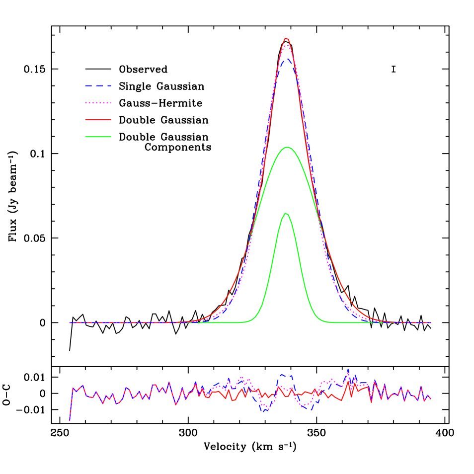
Figure 1: An example spectrum from Sextans A. The error on the points is shown in the upper right corner. This spectrum has a S/N of 37 and is clearly not fit well by a single Gaussian profile. The residuals to the fits are shown in the bottom panel. Both the double Gaussian profile and Gauss-Hermite polynomial statistically fit the observed spectrum better than the single Gaussian profile at the 99.9% confidence level in a single-tailed F-test.

The top panel of Figure 1 shows an extracted spectrum (black) from the VLA-ANGST observations of Sextans A with single Gaussian profile (blue dashed), double Gaussian profile (solid red), and Gauss-Hermite polynomial fits (dotted magenta). The bottom panel shows the residual to the fit. This spectrum has a clear narrow peak that is not fit well by the single Gaussian profile. Both the double Gaussian profile and the Gauss-Hermite polynomial fit the spectrum statistically better than the single Gaussian profile at the 99.9% confidence level. Although the Gauss-Hermite polynomial is a better fit than the single Gaussian profile, the residuals clearly show that the double Gaussian profile is even better.

In summary, we identify cold H I by the following process: 1) only spectra with a S/N greater than 10 were fit, 2) each spectrum was successively fitted with a single and double Gaussian function, 3) each individual component of the double Gaussian fit was required to have a minimum S/N of 3.1, 4) the velocity dispersion plus error had to be greater than the velocity resolution of the data, 5) double Gaussian fits were accepted if they improved the fit over a single Gaussian profile at the 95% or greater confidence level in a single tailed F-test, and 6) cold H I can be described by single or double Gaussian profiles with velocity dispersions less than 6 km s^-1.

3.2 Simulations of Synthetic Spectra

There are two factors which could lead to non-detections of existing cold H I. Cold H I could be missed simply because the column density is too low to reach our S/N requirement, or it could be missed because a higher S/N is required to deblend the cold H I from the warm H I. As a test of our ability to extract multiple components from a given spectrum, we produced three sets of 50,000 uniformly distributed synthetic spectra that spanned the S/N of our sample (10 $\leq$ S/N $\leq$ 60; one set each at 0.65, 1.3, and 2.6 km s^-1 velocity resolution). Each spectrum contained two Gaussian profiles that are representative of the warm and cold H I gas; a “broad” Gaussian with $\sigma_{broad}$ between 8 and 12 km s^-1 and a “narrow” Gaussian with $\sigma_{narrow}$ between 3 and 6 km s^-1. We allowed for an offset of $\pm$2.5 km s^-1 between the line centroids. Velocity offsets larger than 2.5 km s^-1 allow for much higher detection fractions since the spectra become more asymmetric. The observed cold H I line centroids are also very similar to the warm H I line centroids (as discussed in §3.1). For each S/N, we randomized the amplitude of the cold H I Gaussian. We then chose the warm H I Gaussian such that the S/N was conserved. As for the analysis with our observations, each individual component was required to have a S/N $>$ 3.1. A new set of Gaussians was produced if each component did not have a S/N $>$ 3.1. We next added random noise to each spectrum and then passed each randomly generated spectrum through our fitting routine to gauge our recovery rate.

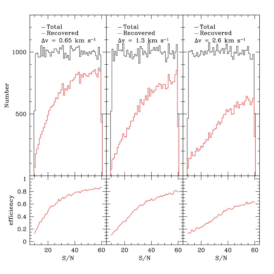
Figure 2: Results from the synthetic spectra containing two Gaussian components randomly generated and processed with our fitting routine. Top Row: The total sample (black) along with the recovered profiles (red; includes best-fit single Gaussian profiles with a velocity dispersion less than 6 km s^-1 for the three different velocity resolutions (0.65, 1.3, and 2.6 km s^-1). Bottom Row: Our recovery efficiency versus S/N for the double Gaussian profiles.

The top row of Figure 2 shows histograms of the total number of synthetic spectra (solid black line) and the total number identified as requiring multiple components by a double Gaussian fit (solid red line) as a function of S/N. The red histograms also include the locations best fit by a single Gaussian with a velocity dispersion of less than 6 km s^-1. The bottom row shows the detection efficiency as a function of S/N for the double Gaussian fits (including the best fit single Gaussians with a velocity dispersion of less than 6 km s^-1). Figure 2 shows that we never identify all double Gaussian profiles within the range of S/N values scrutinized and our recovery efficiency worsens as the velocity resolution decreases. The differences in recovery efficiency between the 0.65 and 1.3 km s^-1 simulations are less pronounced than from 1.3 to 2.6 km s^-1.

Table 2 shows the results of the simulations for each velocity resolution for the double Gaussian profiles that were identified. Column (1) is the velocity resolution, column (2) is the ratio between the input and extracted broad Gaussian amplitude (A_b,sim/A_b,extr), columns (3) and (4) are the average differences between the simulated and extracted broad Gaussian central velocities ($\Delta$v_broad) and velocity dispersions ($\Delta$$\sigma$_broad), column is the ratio between the input and extracted narrow Gaussian amplitude (A_n,sim/A_n,extr), and columns (6) and (7) are the average differences between the simulated and extracted narrow Gaussian central velocities ($\Delta$v_nar) and velocity dispersions ($\Delta$$\sigma$_nar), respectively. These results show that when we do recover two Gaussian profiles, our routines accurately reproduce the input Gaussian parameters.

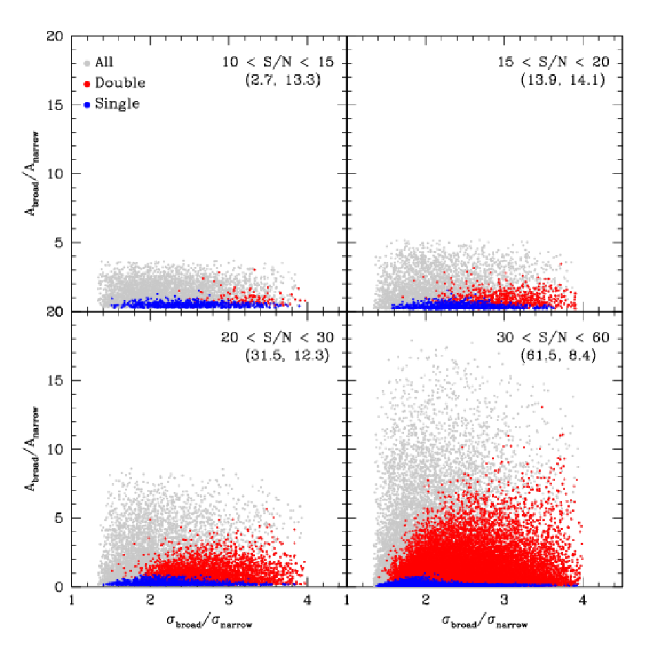
Figure 3: The ratio of the broad and narrow Gaussian amplitudes (A_broad/A_narrow) as a function of the ratio of the broad and narrow velocity dispersions ($\sigma_{\mathrm{broad}}$/$\sigma_{\mathrm{narrow}}$) for the 1.3 km s^-1 velocity resolution simulation in four different S/N bins. The grey dots are all of the simulated spectra. The red dots are those spectra identified as containing two components by our fitting routines, and the blue dots are the simulated spectra that were identified only containing a single Gaussian component with a velocity dispersion of less than 6 km s^-1. The values in the parentheses are the recovery percentages for the best fit double (left) and single (right) Gaussians. We clearly identify more of the spectra at higher S/N values. Our routines have a harder time recovering the two Gaussian components when the velocity dispersions are similar.

In Figure 3 we plot the amplitude ratio of the broad and narrow Gaussian components (A_broad/A_narrow) versus the ratio of the velocity dispersions ($\sigma_{\mathrm{broad}}$/$\sigma_{\mathrm{narrow}}$) for the 1.3 km s^-1 velocity resolution simulation. We show these ratios in four different S/N bins to understand where our fitting routines have trouble identifying the two Gaussian components. The grey points represent all of the simulated spectra, the red points are those spectra identified as containing two Gaussian components, and the blue points are the simulated spectra best fit by a single Gaussian with a velocity dispersion of less than 6 km s^-1 (even though the input spectra contains both a broad and narrow Gaussian as described above). As is shown in Figure 2, the recovery efficiency is dependent upon the S/N. The best fit single Gaussians are predominately in a regime where the narrow component dominates the spectra (amplitude ratios less than 1 and velocity dispersion ratios less than 2.5). We also have difficulty identifying the narrow component when the broad component dominates the spectra in all S/N bins. Lastly, our routines do not pick up multiple components when the velocity dispersions are similar. These plots show some of the complexities in simulating and recovering multiple Gaussian components. When we do identify the spectra as containing multiple components, however, our routines accurately reproduce the input parameters. The simulations indicate that we can be confident of our detections in the observed data. However, the simulations also show that we can only reliably compute lower limits to the cold H I content. A complete census of the cold H I would require both higher S/N spectra and a detailed knowledge of the intrinsic distributions in A_broad/A_narrow and $\sigma_{\mathrm{broad}}$/$\sigma_{\mathrm{narrow}}$ (in order to make incompleteness corrections).

We also produced 50,000 synthetic spectra of single Gaussian profiles to quantify our false positives. These spectra were generated using a velocity dispersion between 8 and 12 km s^-1 with S/N values between 10 and 60. We used a velocity resolution of 2.6 km s^-1 since this gives the worst recovery results. With our acceptance criteria, we failed to find a single false identification of multiple components in our synthetic spectra. We do not start to see the potential for false detections until the confidence level is lowered to $\sim$70%. These simulations give us confidence that our fitting results are robust to false detections.

4 Results

4.1 Cold H I Detections

Each galaxy in our sample varies in terms of the total number of spectra and observed minimum, maximum, and average S/N (and column density). In total, we have analyzed roughly 4,100 independent lines-of-sight. Table 3 summarizes the observed spectral properties of each galaxy. The columns indicate 1) galaxy name, 2) total number of independent lines-of-sight scrutinized (N_t), 3) average S/N of the extracted spectra ($<$S/N$>_{t}$), 4) the approximate column density at a S/N of 10 (N_HI,min), 5) the peak column density (N_HI,peak), and 6) the average column density ($<$N_HI$>$). All of the H I spectra in DDO 82, KDG 73, KK 230, and KKH 98 have S/N values below our threshold and as a result had no spectra analyzed, reducing our final sample to 27 galaxies.

Table 4 summarizes the results of our fitting routine. The columns are described as follows: 1) galaxy name, 2) the average S/N of the spectra where cold H I is found ($<$S/N$>_{c}$), 3) the areal filling factor of the cold H I defined as the ratio of the number of cold H I detections and the total number of scrutinized spectra ($\mathcal{F}_{fill}$), 4) the cold-to-total H I mass fraction defined as the ratio of the total summed column densities of the cold H I Gaussian profiles and the total summed column densities in the areas scrutinized ($\mathcal{F}_{mass}^{low}$), 5) an estimate of the upper limit to the cold-to-total H I mass fraction assuming each line-of-sight contains cold H I ($\mathcal{F}_{mass}^{up}$; see §4.5), 6 & 7) the average velocity dispersion of the narrow and broad Gaussian components ($<$$\sigma_{n}$$>$ and $<$$\sigma_{b}$$>$), and 7) the average velocity dispersion of the locations where a single Gaussian profile was sufficient to describe the spectrum ($<$$\sigma_{s}$$>$). Column 5 also includes all of the best fit single Gaussian profiles with a velocity dispersion of less than 6 km s^-1, while column 7 excludes them.

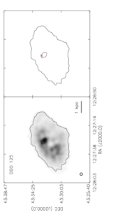
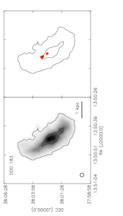
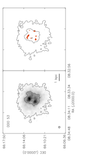
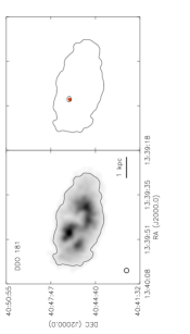
Figure 4: Left: The total H I integrated intensity map. Right: The cold H I locations best described by a double Gaussian (red) and single Gaussian (blue). The contours for all panels represent the $10^{20}$ and $10^{21}$ cm^-2 column density levels. The scale bar at the bottom right denotes a linear size of 1 kpc. The 200 pc beam is shown at the lower left.

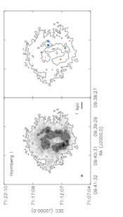
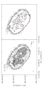
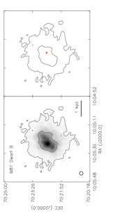
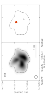
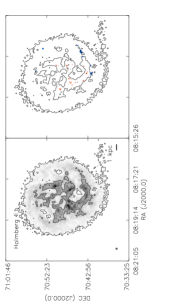
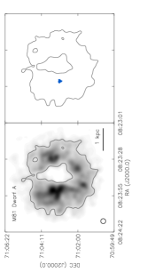
Figure 4: Continued…

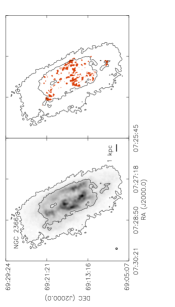
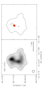
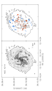
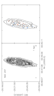
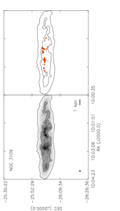
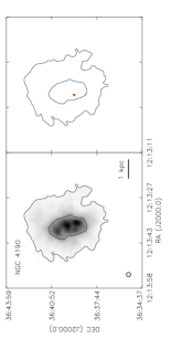
Figure 4: Continued…

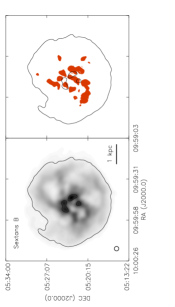
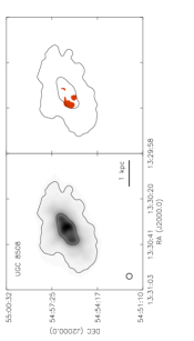
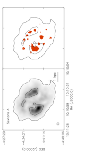
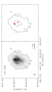
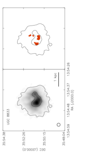
Figure 4: Continued…

We detected cold H I in 23 out of the 27 galaxies in our final sample. Figure 4 shows the spatial distribution of the cold H I for each galaxy. The left panels show the total integrated H I intensity maps with contours of 10²⁰ and 10²¹ cm^-2 overlaid. The right panels have the H I surface density contours overlaid on the locations of the cold H I emission. The majority of the cold H I is clumped in localized regions. Typically, the cold H I is not spatially coincident with the very highest peaks in the total H I distribution in a given galaxy, although it is mainly concentrated in locations where the total H I column density exceeds the canonical threshold for star formation of $\sim$10²¹ cm^-2 (Skillman, 1987). Cold H I described in each of the previous studies also shows a preference for being located in regions of high column density, but not necessarily associated with the highest H I columns. The concentration of the cold H I in these regions is not unexpected given these location have the highest S/N values. The four galaxies in which we do not detect cold H I (DDO 99, MCG09-20-131, NGC 3741, and UGCA 292) show no distinguishing characteristics to give us insight as to why they are non-detections. Each of their total H I masses, M_B values, distances, stellar disk sizes, and star formation rates (see §4.7) are similar to other galaxies in our sample that do show cold H I detections.

4.2 Comparison with Previous Work

Fortunately, our sample of 27 galaxies had some overlap with previous studies using similar methods to detect cold H I. Young et al. (2003) detected cold H I in UGCA 292 and GR8 using the VLA while Begum et al. (2006) detected it in DDO 53, MCG09-20-131, GR8 and M81 Dwarf A using the GMRT. These five galaxies are amongst the faintest and smallest galaxies in our sample and as a result, we detected cold H I in only 3 of these 5 galaxies: DDO 53, GR8, and M81 Dwarf A. Our selection criteria failed to produce a cold H I signature in UGCA 292 or MCG09-20-131.

The three galaxies in which we did detect cold H I are included in Figure 4. For GR8, Young et al. (2003) and Begum et al. (2006) each found cold H I in both the northern and south-western portions of the galaxy while Young et al. (2003) also found some evidence in the eastern portion of the galaxy. In contrast, we only found cold H I in the northern region of GR8. For M81 Dwarf A we detect cold H I only in the eastern side of the galaxy while Begum et al. (2006) find a hint of cold H I in the western side of the galaxy as well. For DDO 53 we found good overall agreement with the previous study, although our total detection area is smaller.

The data quality between each survey is similar, yet they provide minor differences in their results. Our simulations suggest velocity resolution differences may play a role in the detection differences between the studies. The velocity resolutions in our sample for these galaxies are 0.65, 1.3, and 2.6 km s^-1 for GR8, M81 Dwarf A, and DDO 53, respectively. The literature velocity resolutions are 1.3 and 1.65 km s^-1 for GR8, 1.65 km s^-1 for M81 Dwarf A, and 1.65 km s^-1 for DDO 53. The galaxy with the most similar cold H I distribution, DDO 53, has the worst velocity resolution in our sample, 0.85 km s^-1 worse than the literature value. GR8 has been analyzed with three different velocity resolutions and each study finds slightly different results. We reduced our velocity resolution to 1.3 km s^-1 for GR8 to compare to the other studies and obtained no difference in our results. M81 Dwarf A was analyzed with similar velocity resolutions, yet there still exists slight differences. Despite analyzing data from different observatories with different velocity resolutions, the general results are all similar. It seems likely that the differences in each galaxy arise from small differences in the selection criteria and beam shape. For example, both Young et al. (2003) and Begum et al. (2006) used naturally weighted data cubes which, on average, produce higher S/N spectra. However, as noted in §2, the robust weighting for combined array data is ideal for studying extended emission due to the better clean beam approximation of the dirty beam in the CLEAN algorithm. The previous studies also used a cutoff of 90% in the F-test statistic and also allow the narrow Gaussian component to be larger than 6 km s^-1, finding values up to $\sim$8 km s^-1.

4.3 Are the Cold H I Non-Detections Significant?

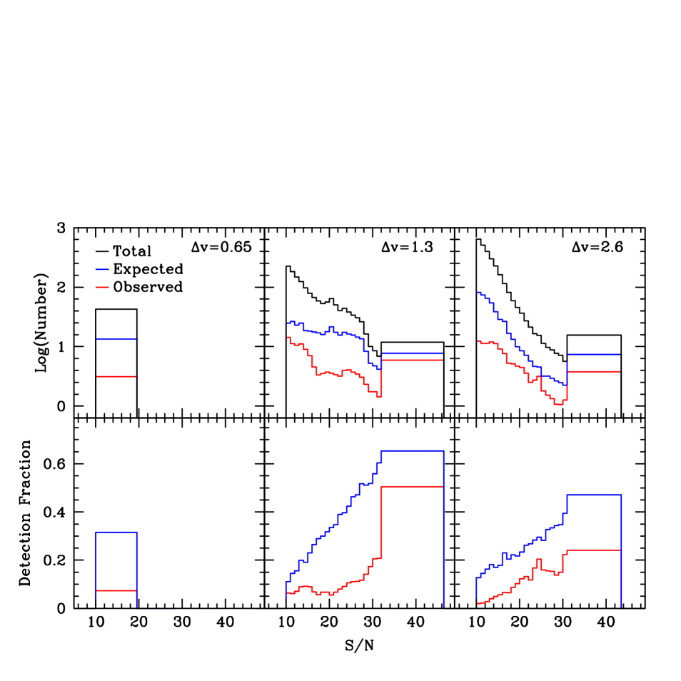
Figure 8: Top: Histograms of the total observed sample for all galaxies (black), the expected number of cold H I detections given our detection efficiency and assuming every line-of-sight contained multiple components (blue), and the actual number of cold H I detections (red) as a function of S/N for each velocity resolution. The histogram bins were chosen such that each contains at least one independent line-of-sight. The large gap between the blue and red histograms demonstrates the cold H I identified with this technique is not ubiquitous. Bottom: The detection fraction as a function of S/N.

If each spectrum consisted of both a broad and narrow component and were not inherently a single Gaussian profile, we would expect to find far more locations with a narrow line signature than we actually do. The top panel of Figure 8 shows a histogram for every independent line-of-sight (black line), the expected number of identified narrow line detections (blue) (based upon our detection efficiency as calculated in §3.2 and the assumption that a narrow component exists at each location), and the actual number of narrow line detections (red) as a function of S/N. The bottom panel shows the detection fraction as a function of S/N. Figure 8 demonstrates the large gap between the number of spectra for which we are sensitive to the presence of narrow H I and the number of spectra for which there are detections. Our expected recovery fraction is insensitive to small changes in the reasonable ranges used for the parameters.

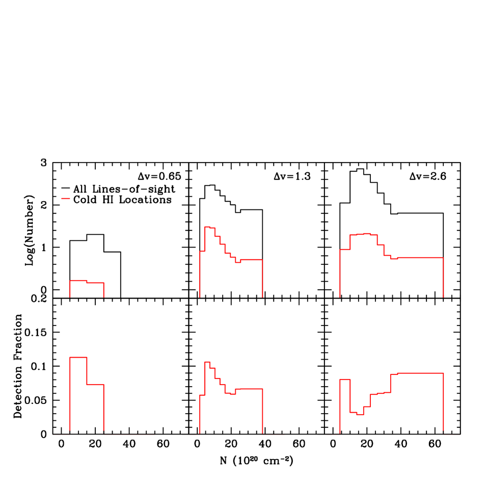
Figure 9: Top: Histograms of observed column densities of our entire sample (black) and where we find cold H I for each velocity resolution. Bottom: The detection fraction as a function of column density. Our detection fractions are relatively constant across all column densities observed.

The lower S/N spectra have fewer fractional detections. As discussed in §3.2, the lower fractional detections at lower S/N values are due, in part, to our recovery efficiency but may also be due to a minimum total H I column density required for the appearance of cold H I. Kanekar et al. (2011) recently observed H I in the Milky Way and determined a minimum column density threshold of 2$\times$10²⁰ cm^-2 for the formation of a cold phase of H I, which is just at the column density limit of where our sample begins. The top row of Figure 9 shows histograms of all of the observed column densities in our galaxy sample (black), and the column densities where we detect cold H I (red). The bottom row shows our detection fraction as a function of column density.

The small fraction of narrow line detections at high S/N compared to what would be expected clearly shows that the cold H I that can be identified with this technique is inconsistent with a ubiquitous distribution. It should also be noted that there could exist cold H I at every line-of-sight below a S/N of 3.1 that we would be insensitive to. However, it would be unphysical for the presence of gas to be related to our S/N criterion and not to the H I column density. Furthermore, absorption line studies in the Milky way indicate that cold H I gas is not ubiquitous (e.g., Begum et al. 2010; Kanekar et al. 2011).

4.4 The Velocity Dispersions of Cold and Warm H I

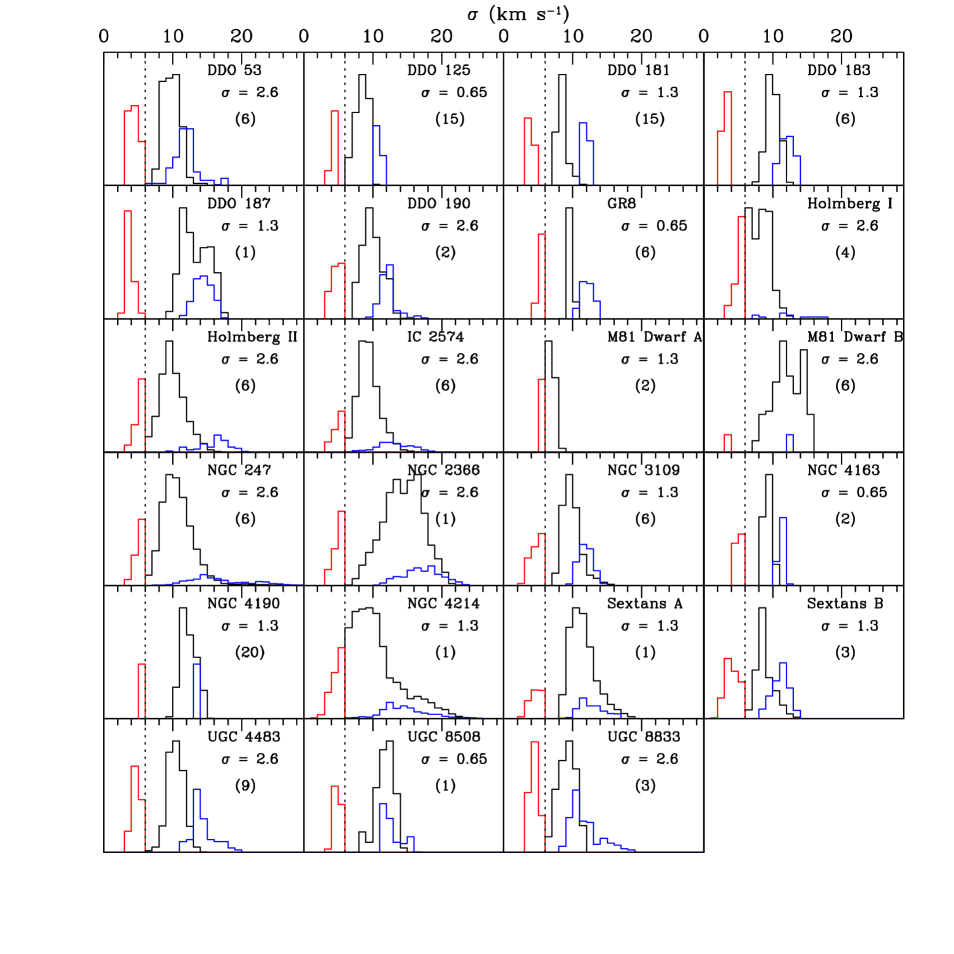
Figure 10: Histograms of the velocity dispersions of the best fit single Gaussian profiles (black), narrow component (red), and broad component (blue). The single Gaussian profile distributions have been scaled down by the number in the parentheses in order to discern the other two components. The dashed vertical line denotes our narrow-line cutoff of 6 km s^-1. The velocity resolution ($\sigma$) is listed below the galaxy names. Typically, the broad component velocity dispersions overlap with the single Gaussian profile velocity dispersions indicating they arise from the same gas phase.

The typical velocity dispersion for the cold H I is $\sim$4.5 km s^-1. The broad components and best-fit single Gaussian profiles vary by galaxy, but they generally have similar values. We expect the broad and best fit single components to be similar if they are both tracing the same warm H I. Figure 10 shows histograms of the narrow (red), broad (blue), and single (black) velocity dispersions for each galaxy. The dotted vertical line denotes our cold H I cutoff limit of 6 km s^-1. The single component histograms have been scaled in order to show the narrow and broad component histograms more clearly. Generally, the velocity dispersions of the broad components overlap with those of the single components. However, the peak in the broad component is offset from the peak in the single component towards higher values. This behavior is also seen for the majority of the cases in the literature, and is probably due to the fact that it is easier to identify a narrow component when the broad component has a much larger value.

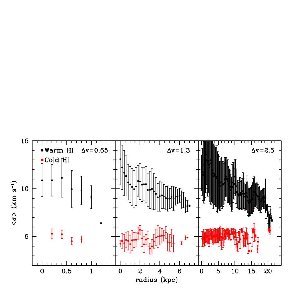
Figure 11: The average velocity dispersion, $<$$\sigma$$>$, as a function of radius for the warm (black) and cold (red) H I gas for each of our velocity resolutions. We have omitted the locations best fit by a single Gaussian with a velocity dispersion of less than 6 km s^-1. The averages are taken over 200 pc bins (the beam size). The error bars are the dispersions of the values in the bins. The velocity of the warm component decreases with radius indicating a possible decrease in turbulence as the radius increases from the main stellar body. Some of the errorbars at large radii for the 2.6 km s^-1 velocity resolution overlap with values below our 6 km s^-1 cutoff. This is due to the dispersions being affected by a few larger values in these bins.

In Figure 11, we plot the average velocity dispersion, $<$$\sigma$$>$, of the warm (black) and cold (red) H I gas as a function of radius for each of our different velocity resolutions. We have omitted the locations best fit by a single Gaussian with a velocity dispersion of less than 6 km s^-1. The average warm H I velocity dispersion declines with radius. This trend is similar to the total H I velocity dispersion versus radius seen by Tamburro et al. (2009). The decrease in the velocity dispersion with increasing radius may indicate a decrease in turbulent energy supplied by the underlying stellar population as the radius increases away from the center of the stellar disk.

4.5 The Areal and Mass Fractions of Cold H I

Recent work on galaxy simulations of spiral disks have put limits on the predicted volume filling factor of the different gas phases in the ISM (e.g., de Avillez & Breitschwerdt 2004). The cold (T $<$ 1000 K) ISM occupies $\lesssim$20% of a galaxy’s volume, depending upon the star formation (supernova) rate. The cold neutral medium, however, may occupy only a few percent of the volume (McKee & Ostriker, 1977). The actual value will vary by galaxy and must also be sensitive to the available ISM coolants (e.g., C$+$, CO, dust, etc.) and the global gravitational potential.

Without knowing the exact 3-dimensional structure of the galaxies in our sample, we cannot calculate the volume filling fractions. Instead, we calculate the areal filling fractions ($\mathcal{F}_{fill}$), i.e., the ratio of the number of lines-of-sight with detected cold H I and the total number of lines-of-sight with S/N $>$ 10 (see Table 4, column 3). We derive an average $\mathcal{F}_{fill}$ value of 9%. The true volume filling fractions based upon our detections are most likely even lower than these values since the scale height of the warm H I will be larger than that of the cold H I. The low filling fractions we compute are consistent with the ISM model of McKee & Ostriker (1977).

We also computed a lower limit to the total mass (flux) contribution of the cold H I for each galaxy using the narrow component of the Gaussian fits ($\mathcal{F}_{mass}^{low}$; see Table 4, column 4). Young & Lo (1996, 1997) and de Blok & Walter (2006) found that roughly 20% of the total H I mass is in the cold H I, which is significantly higher than the $\sim$3% typical for our values of $\mathcal{F}^{low}_{mass}$. It is unclear as to the reason for this large discrepancy since the data are of similar quality. The biggest differences may lie in the higher S/N resulting from the natural weighting these other studies use as compared to the robust weighting we employ. Also, de Blok & Walter use a different statistical test in defining the acceptance of cold H I detections. These authors accept a double Gaussian fit as statistically better than a single Gaussian fit if the $\chi$² value is improved by 10%. Furthermore, our values are lower limits given our selection criteria and sensitivities. Figure 12 plots $\mathcal{F}_{fill}$ and $\mathcal{F}_{mass}^{low}$ as a function of M_B (left) and $M_{HI}$ (right). No obvious trends arise between the areal filling fraction and mass fraction with absolute $B$-band magnitude or total H I mass.

If we assume (as noted in §4.3) that each line of sight has cold H I just below our detection limits, we can estimate an upper limit to the amount of cold H I in each galaxy. To do this we have used a representative cold H I Gaussian of amplitude 3.1$\sigma$ and velocity dispersion of 4.5 km s^-1 at each location where we do not detect cold H I. We then add this “extra” mass to our detected cold H I mass to produce an upper limit to the cold H I mass fraction ($\mathcal{F}_{mass}^{up}$; see column 5 in Table 4). These values of $\mathcal{F}^{up}_{mass}$ can range up to 50%. However, since the cold H I is most frequently associated with higher values of N_HI (see §4.1), it is unlikely that the true values of cold H I mass get as high as these upper limits.

Another, perhaps more reasonable way to calculate an upper limit to the cold-to-total H I mass fraction is to find the typical fractional flux contributed to the cold component along each line-of-sight and assume this fraction holds throughout the sample. For locations where we find both warm and cold H I components, the cold H I typically is not the dominant phase in the ISM. The top row of Figure 13 shows a normalized histogram of the flux ratio of cold and total H I defined as the ratio of the column density of the narrow Gaussian profile and the total column density along the line-of-sight. The cold H I constitutes $\sim$20% of the total line flux for any given line-of-sight. The bottom panels of Figure 13 show this same ratio as a function of S/N for each velocity resolution. If we assume that every line-of-sight contains cold H I, then an upper limit to the cold-to-total mass ratio for each galaxy is $\sim$20%. This value is what is reported by Young & Lo (1996, 1997) and de Blok & Walter (2006). However, this value is also likely too high since it requires the entire galaxy to contain cold H I gas. Dickey et al. (2000) observed the Small Magellanic Cloud in 21 cm absorption and found that the mass fraction of cold H I to be less than 15% of the total H I content. It seems likely that the true value of the cold H I mass fractions of the low mass galaxies in our sample are between our lower limits and $\sim$15%.

Begum et al. (2010) observed 21-cm Milky Way absorption towards 12 background radio continuum sources. They were able to determine the flux contribution of the cold H I along many of these sight lines. They find that the cold H I contributes from a low of $\sim$2% to as high as $\sim$69%, of the total flux determined in the same manner, with a median of $\sim$30%. While a direct comparison between the optically thick cold H I observed by Begum et al. (2010) and our optically thin emission is not obvious, we would not expect the fraction of cold H I in emission to be drastically different. Our result of $\sim$20% is slightly lower than their median value, but does not appear to be at odds with their result.

4.6 Cold H I Locations that Lack a Warm Component

As discussed in §3.1, some lines-of-sight were best fit by a single Gaussian profile with a velocity dispersion of less than 6 km s^-1. These best fit single Gaussian profiles were found in 6 of the 23 galaxies with cold H I detections. Most of these six galaxies have a large fraction of their H I at galactocentric radii beyond the $\sim$25 mag arcsec^-2 optical level, and the majority of these single Gaussian fits are also located at larger radii. Figure 14 shows the radial distribution of the cold H I locations that lack a warm component. The galaxies have been ordered from low (M81 Dwarf A) to high (NGC 247) absolute $B$-band luminosity. Two of these galaxies, M81 Dwarf A and Holmberg I, have large central holes in their H I distributions (see Warren et al. 2011 and references therein) where much of their gas is pushed beyond the optical radius. Only NGC 247 has a majority of these locations within the optical radius.

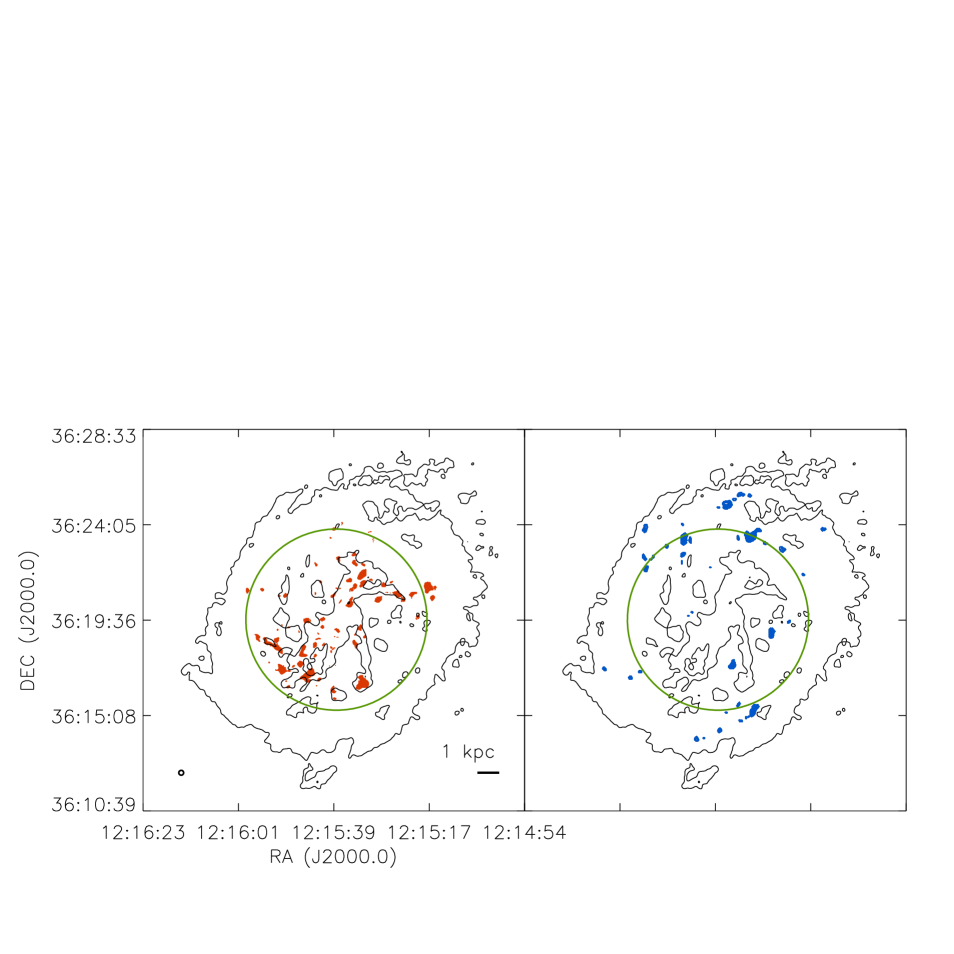
Figure 15: Left: The cold H I distribution (red) of NGC 4214 for those locations best fit by double Gaussians profiles only. Right: The cold H I distribution (blue) for those locations best fit by single Gaussian profiles with velocity dispersions less than 6 km s^-1 only. The contours represent the 10²⁰ and 10²¹ cm^-2 total H I column densities. The green circle approximates the 25 mag arcsec^-2 optical level. The beam is shown at lower left. The majority of the cold H I detections described by a single Gaussian profile are outside of the bulk of the stellar distribution.

Figure 15 shows an example of the difference between those areas that contain a warm component and those that lack one for NGC 4214. The left panel shows only those locations that contain both a warm and cold H I component while the right panel also includes the locations that lack a warm component. The contours correspond to the 10²⁰ and 10²¹ cm^-2 total H I column densities and the blue circle approximates the 25 mag arcsec^-2 level (uncorrected for inclination and position angle). It is immediately apparent that the majority of the best fit single Gaussian profiles fall well beyond the bulk of the stellar population and far from any heat sources. Tamburro et al. (2009) provides evidence that the warm H I velocity dispersions inside the optical radius of disk galaxies is driven by stellar processes, while areas beyond the optical radius may be driven by thermal broadening and/or magneto-rotational instabilities. These authors also point out that the velocity dispersions decline as a function of radius, falling below the typical 10 km s^-1 beyond the optical radius. We also see this declining trend in the velocity dispersion with radius (see Figure 11). These results are suggestive that cold H I can be the dominant constituent of the ISM only in the lower UV radiation field beyond the $\sim$25 mag arcsec^-2 optical level.

4.7 Comparing the Cold H I Gas Mass with Molecular Gas Masses and Star Formation Rates

We next compare the cold H I gas masses to the molecular gas masses and star formation rates (SFRs) in each galaxy. To make these comparisons we compute the SFRs and estimate the amount of molecular hydrogen each galaxy contains. The relationship between the SFR and molecular hydrogen is discussed in detail in §1. We used the SFRs given by both FUV and H$\alpha$ luminosities to estimate the amount of molecular hydrogen.

Table 5 lists the SFRs derived from FUV and H$\alpha$ luminosities taken from the literature for each galaxy with a detected cold H I signature. The columns are: (1) galaxy name, (2) mass of the cold H I ($M_{coldHI}$) computed using the lower limit mass fraction from Table 4 multiplied by the total H I mass given in Table 1, (3) apparent FUV magnitude (m_FUV; Lee et al. 2011), (4) the logarithm of the FUV luminosity (L_FUV), (5) the FUV SFR (SFR_FUV) computed using the relation given in Salim et al. (2007), (6) the H₂ gas mass ($M_{H_{2}}^{FUV}$) computed from SFR_FUV assuming a 100 Myr timescale and a star formation efficiency of 10% ($M_{H_{2}}^{FUV}$ = SFR_FUV $\times$ 100 Myr / 0.1), (7) the approximate fraction of the cold ISM attributed to the cold H I ($\mathcal{M}_{FUV}$) defined as $M_{coldHI}$/($M_{coldHI}$ + $M_{H_{2}}^{FUV}$), (8) the logarithm of the H$\alpha$ luminosity (L_Hα; Kennicutt et al. 2008), (9) the SFR derived from L_Hα using the relation in Kennicutt (1998), (10) the H₂ gas mass ($M_{H_{2}}^{H\alpha}$) computed from SFR_Hα assuming a 5 Myr timescale and a star formation efficiency of 10% ($M_{H_{2}}^{H\alpha}$ = SFR_FUV $\times$ 5 Myr / 0.1), and (11) the approximate fraction of the cold ISM attributed to the cold H I ($\mathcal{M}_{H\alpha}$) defined as $M_{coldHI}$/($M_{coldHI}$ + $M_{H_{2}}^{H\alpha}$). Using our lower limit mass fraction from the spectra above S/N of 10 and extrapolating it over the entire galaxy provides a lower limit to the total cold H I mass.

The expected relationship between the currently observed cold H I and the computed molecular gas masses is not immediately clear. The mass fractions of the cold ISM attributed to the cold H I is lower for H₂ masses computed from the longer timescale SFR_FUV (Table 5, column 7) than they are for those computed from SFR_Hα (Table 5, column 11). The time scale to convert the cold H I into molecular hydrogen is likely dependent upon the metallicity of the environment (a longer time scale is expected for lower metallicities) and local UV radiation field (a shorter time scale is expected for lower UV radiation). Since dwarf galaxies have both low metallicities and different ranges of UV radiation strengths, it is not obvious which molecular gas mass estimate provides the best comparison. Unfortunately, our current data do not allow us to investigate these timescales further.

The top and bottom panels of Figure 16 show plots of the SFR_FUV (filled circles) and SFR_Hα (open squares) as a function of the cold H I mass and total H I mass, respectively. If the cold H I is related to the star formation in any direct way, we would expect to find a trend in this relation. Indeed, the higher the cold H I gas mass, the higher the SFR, although this same trend is seen with the total H I gas mass and may just be a consequence of the more H I gas available, the higher the SFR. The middle panel shows the SFR efficiency (SFE_HI) defined as the SFR divided by the total H I gas mass as a function of the cold H I gas mass. The SFE_HI is roughly constant over our range of cold H I masses. The differences between the derived FUV and H$\alpha$ star formation rates has been previously reported in Lee et al. (2009) and is due at least in part to the fact that the SFRs are averaged over different timescales. Environmental conditions may also influence SFR_Hα by leakage of the ionizing photons from the star forming regions (see Relano et al. 2012 for details).

We can compare our molecular gas mass estimates derived from the SFRs to a direct observational estimate of the molecular gas in NGC 4214 (Walter et al., 2001) to see if our values are reasonable. These authors observed CO emission in the inner $\sim$1$\farcm$6$\times$1$\farcm$6 of the star forming disk of NGC 4214 (an area much smaller than the H I disk, see §4.6) and derived a molecular gas mass of 5.1$\times$10⁶ $M_{\odot}$. This value is similar to the molecular gas mass estimate we get from SFR_Hα of 6.1$\times$10⁶ $M_{\odot}$. The molecular gas mass value computed by Walter et al. was based on an assumed CO to H₂ conversion factor (the so called ’X-factor’) derived from observations of Galactic environments (i.e., high metallicity). Recent work on the X-factor has shown that the relation changes with decreasing mean visual extinction (e.g., Leroy et al. 2009; Glover & Mac Low 2011; Schruba et al. 2012). The lower metallicity environment of dIrr galaxies results in lower visual extinction values and thus a different X-factor value. Depending upon the true mean visual extinction value of NGC 4214, the actual molecular gas mass could be higher by a factor of a few to an order of magnitude or more. Schruba et al. (2012) derive an X-factor value roughly 40 times higher than the Galactic value for NGC 4214. Using this value, the Walter et al. (2001) molecular gas mass increases to $\sim$2$\times$10⁸ $M_{\odot}$, closer to our derived H₂ mass using SFR_FUV of 1$\times$10⁸ $M_{\odot}$. Schruba et al. (2012) also derive a molecular gas mass of $\sim$2$\times$10⁸ $M_{\odot}$ for NGC 4214. The factor of 2 difference between the values most likely arise from our basic assumptions of a timescale of 100 Myr for the FUV emission and/or the star formation efficiency of 10%. Unfortunately, the lack of CO detections for the few galaxies in our sample that have been observed for CO prohibit us from repeating this exercise for other galaxies in our sample (e.g., Israel et al. 1995; Verter & Hodge 1995; Leroy et al. 2009; Schruba et al. 2012). Nevertheless, our estimates of molecular gas masses, although uncertain, are not unreasonable. Direct comparisons between the CO detections in NGC 4214 and our cold H I detections is the focus of future work.

5 Conclusions

We have observed line-of-sight H I emission spectra in 31 nearby, low metallicity dIrr galaxies in order to search for cold H I defined by a velocity dispersion of less than 6 km s^-1. We have detected it in 23 of 27 galaxies after quality control cuts were applied. The cold H I may be the future sites of molecular cloud and star formation and to date, are the only way to potentially trace star forming gas at low metallicity. Based upon our observations, we find:

• The cold H I gas is found in localized regions and usually at total H I column densities above the canonical threshold of star formation of 10²¹ cm^-2 (Skillman, 1987). The cold H I in a given galaxy is also not typically associated with the very highest surface density gas (see Figures 4 & 9).

• The cold H I has a typical velocity dispersion of $\sim$4.5 km s^-1 (T $\lesssim$ 800 K).

• We derive an average value to the volume filling fraction of the cold H I of 9% (assuming our lower limit detections).

• We find lower limits to the cold H I gas mass fractions of a few percent, consistent with some models of the multi-phase ISM (McKee & Ostriker, 1977).

• The SFE_HI is roughly constant as a function of the total cold H I mass over the observed gas mass ranges.

• The cold H I contributes $\sim$20% of the line-of-sight flux in locations where we detect both a cold and warm component.

• Cold H I gas that lacks a warm component is typically found at radii larger than the 25 mag arcsec^-2 optical radius.

Future work will investigate the relationship between the cold H I, local ISM conditions, and tracers of current star formation.

Table 1: Observed Galaxy Properties

1	2	3	4	5	6	7	8	9	10	11
Galaxy	RA	DEC	Da	$M_{\mathrm{HI}}$	MB	$a^{b}$	ib	Beam Size	$\Delta$ v	rmsnoise
	(J2000.0)	(J2000.0)	(Mpc)	(107 $M_{\odot}$)		(′)	(deg)	(″)	(km s-1)	(mJy beam-1)
DDO 53	$08^{h}34^{m}07\fs 2$	$+66{\arcdeg}10{\arcmin}54{\arcsec}$	3.61	6.2	-13.45	1.6	30	11.43	2.6	0.8
DDO 82	$10^{h}30^{m}35\fs 0$	$+70{\arcdeg}37{\arcmin}10{\arcsec}$	3.80	0.3	-14.44	3.4	55	10.86	1.3	1.7
DDO 99	$11^{h}50^{m}53\fs 0$	$+38{\arcdeg}52{\arcmin}50{\arcsec}$	2.59	4.7	-13.37	4.1	71	15.93	1.3	2.0
DDO 125	$12^{h}27^{m}41\fs 8$	$+43{\arcdeg}29{\arcmin}38{\arcsec}$	2.58	2.9	-14.04	4.3	58	15.99	0.65	3.0
DDO 181	$13^{h}39^{m}53\fs 8$	$+40{\arcdeg}44{\arcmin}21{\arcsec}$	3.14	2.4	-12.94	2.3	57	13.14	1.3	1.6
DDO 183	$13^{h}50^{m}51\fs 1$	$+38{\arcdeg}01{\arcmin}16{\arcsec}$	3.22	2.0	-13.08	2.2	75	12.81	1.3	1.5
DDO 187	$14^{h}15^{m}56\fs 5$	$+23{\arcdeg}03{\arcmin}19{\arcsec}$	2.21	1.2	-12.43	1.7	42	18.67	1.3	2.1
DDO 190	$14^{h}24^{m}43\fs 5$	$+44{\arcdeg}31{\arcmin}33{\arcsec}$	2.79	4.1	-14.14	1.8	28	14.78	2.6	0.7
GR8	$12^{h}58^{m}40\fs 4$	$+14{\arcdeg}13{\arcmin}03{\arcsec}$	2.08	0.6	-12.00	1.1	25	19.83	0.65	4.4
Holmberg I	$09^{h}40^{m}32\fs 3$	$+71{\arcdeg}10{\arcmin}56{\arcsec}$	3.90	14.6	-14.26	3.6	37	10.58	2.6	1.2
Holmberg II	$08^{h}19^{m}05\fs 0$	$+70{\arcdeg}43{\arcmin}12{\arcsec}$	3.38	56.6	-16.57	7.9	31	12.20	2.6	1.5
IC 2574	$10^{h}28^{m}27\fs 7$	$+68{\arcdeg}24{\arcmin}59{\arcsec}$	3.80	123.9	-17.17	13.2	68	10.86	2.6	0.9
KDG 73	$10^{h}52^{m}55\fs 3$	$+69{\arcdeg}32{\arcmin}45{\arcsec}$	4.03	0.05	-10.75	0.6	35	10.24	0.65	2.0
KK 230	$14^{h}07^{m}10\fs 7$	$+35{\arcdeg}03{\arcmin}37{\arcsec}$	1.97	0.07	-8.49	0.6	35	20.94	0.65	3.8
KKH 98	$23^{h}45^{m}34\fs 0$	$+38{\arcdeg}43{\arcmin}04{\arcsec}$	2.54	0.3	-10.29	1.1	58	16.24	0.65	2.8
M81 Dwarf A	$08^{h}23^{m}55\fs 1$	$+71{\arcdeg}01{\arcmin}56{\arcsec}$	3.44	1.2	-11.37	1.3	24	11.99	1.3	0.9
M81 Dwarf B	$10^{h}05^{m}30\fs 6$	$+70{\arcdeg}21{\arcmin}52{\arcsec}$	5.3b	2.7	-14.23	0.9	49	7.78	2.6	0.6
MCG09-20-131	$12^{h}15^{m}46\fs 7$	$+52{\arcdeg}23{\arcmin}15{\arcsec}$	1.6c	1.2	-12.36	1.2	77	25.78	1.3	3.3
NGC 247	$00^{h}47^{m}08\fs 3$	$-20{\arcdeg}45{\arcmin}36{\arcsec}$	3.52	110.6	-17.92	21.4	72	11.72	2.6	1.3
NGC 2366	$07^{h}28^{m}53\fs 4$	$+69{\arcdeg}12{\arcmin}51{\arcsec}$	3.21	56.7	-15.85	7.3	72	12.85	2.6	1.0
NGC 3109	$10^{h}03^{m}07\fs 2$	$-26{\arcdeg}09{\arcmin}36{\arcsec}$	1.27	27.0	-15.18	19.7	86	32.48	1.3	8.5
NGC 3741	$11^{h}36^{m}06\fs 4$	$+45{\arcdeg}17{\arcmin}07{\arcsec}$	3.24	8.1	-13.01	2.0	58	12.73	1.3	2.1
NGC 4163	$12^{h}12^{m}08\fs 9$	$+36{\arcdeg}10{\arcmin}10{\arcsec}$	2.87	0.9	-13.76	1.9	34	14.37	0.65	2.2
NGC 4190	$12^{h}13^{m}44\fs 6$	$+36{\arcdeg}38{\arcmin}00{\arcsec}$	3.5b	4.5	-14.20	1.7	29	11.79	1.3	1.5
NGC 4214	$12^{h}15^{m}39\fs 2$	$+36{\arcdeg}19{\arcmin}37{\arcsec}$	3.04	41.2	-17.07	8.5	40	13.57	1.3	1.1
Sextans A	$10^{h}11^{m}00\fs 8$	$-04{\arcdeg}41{\arcmin}34{\arcsec}$	1.38	6.2	-13.71	5.9	35	29.89	1.3	4.5
Sextans B	$10^{h}00^{m}00\fs 1$	$+05{\arcdeg}19{\arcmin}56{\arcsec}$	1.39	4.2	-13.88	5.1	48	29.68	1.3	2.0
UGCA 292	$12^{h}38^{m}40\fs 0$	$+32{\arcdeg}46{\arcmin}00{\arcsec}$	3.62	4.0	-11.36	1.0	47	11.40	0.65	2.1
UGC 4483	$08^{h}37^{m}03\fs 0$	$+69{\arcdeg}32{\arcmin}45{\arcsec}$	3.41	3.3	-12.58	1.2	56	12.10	2.6	0.8
UGC 8508	$13^{h}30^{m}44\fs 4$	$+54{\arcdeg}54{\arcmin}36{\arcsec}$	2.58	1.9	-12.95	1.7	55	15.99	0.65	2.3
UGC 8833	$13^{h}54^{m}48\fs 7$	$+35{\arcdeg}50{\arcmin}15{\arcsec}$	3.08	1.3	-12.31	0.9	28	13.39	2.6	0.6

^aDalcanton et al. (2009); ^bKarachentsev et al. (2004); ^cMCG09-20-131 may have a greater distance than indicated due to ambiguities in measuring the TRGB.

Table 2: Simulated Spectra Results

1	2	3	4	5	6	7
Velocity	Ab,sim/Ab,extr	$\Delta$vbroad	$\Delta$$\sigma$broad	An,sim/An,extr	$\Delta$vnar	$\Delta$$\sigma$nar
Resolution		(km/s)	(km/s)		(km/s)	(km/s)
0.65	1.0$\pm$0.1	0.0$\pm$0.3	0.0$\pm$0.6	1.0$\pm$0.1	0.0$\pm$0.2	0.0$\pm$0.3
1.30	1.0$\pm$0.2	0.0$\pm$0.5	0.0$\pm$0.7	1.0$\pm$0.1	0.1$\pm$0.2	0.1$\pm$0.3
2.60	1.0$\pm$0.2	-0.2$\pm$0.8	0.0$\pm$0.9	1.0$\pm$0.1	0.5$\pm$0.4	0.1$\pm$0.5

Table 3: Individual Galaxy Properties

1	2	3	4	5	6
Galaxy	Nt	$<$S/N$>_{t}$	NHI,min	NHI,peak	$<$NHI$>$
			(1019 cm-2)	(1021 cm-2)	(1020 cm-2)
DDO 53	48	14.8	6.76	3.19	16.0
DDO 82	0	$\cdots$	19.20	$\cdots$	$\cdots$
DDO 99	19	12.7	14.28	2.38	13.0
DDO 125	6	10.8	14.07	1.62	11.3
DDO 181	9	11.2	13.69	1.53	11.3
DDO 183	11	11.9	11.78	1.97	14.1
DDO 187	13	14.8	7.78	2.59	14.0
DDO 190	46	20.6	3.86	3.55	15.8
GR8	3	10.7	12.97	1.06	9.23
Holmberg I	24	11.1	11.84	2.47	16.6
Holmberg II	207	12.0	11.11	3.82	18.1
IC 2574	1026	13.1	8.43	4.83	15.8
KDG 73	0	$\cdots$	27.69	$\cdots$	$\cdots$
KK 230	0	$\cdots$	10.77	$\cdots$	$\cdots$
KKH 98	0	$\cdots$	15.55	$\cdots$	$\cdots$
M81 Dwarf A	3	10.7	6.91	0.64	5.67
M81 Dwarf B	9	11.8	10.93	3.53	22.9
MCG09-20-131	3	14.0	7.16	1.97	12.7
NGC 247	848	12.9	15.10	5.24	22.6
NGC 2366	511	16.2	6.54	6.83	21.0
NGC 3109	404	17.6	10.49	3.83	13.0
NGC 3741	9	11.0	17.62	3.07	22.0
NGC 4163	4	11.1	13.89	1.48	11.1
NGC 4190	20	12.0	14.63	3.32	22.6
NGC 4214	488	12.6	6.60	3.26	10.5
Sextans A	133	16.5	6.53	4.02	10.2
Sextans B	173	17.0	2.65	1.41	4.40
UGCA 292	20	12.0	24.97	3.55	23.6
UGC 4483	28	14.9	7.53	2.92	15.1
UGC 8508	12	13.1	11.42	2.47	16.8
UGC 8833	16	16.6	4.38	2.21	12.0

Table 4: Individual Galaxy Results

1	2	3	4	5	6	7	8
Galaxy	$<$S/N$>_{c}$	$\mathcal{F}_{fill}$	$\mathcal{F}_{mass}^{low}$	$\mathcal{F}_{mass}^{up}$	$<$$\sigma_{n}$$>$	$<$$\sigma_{b}$$>$	$<$$\sigma_{s}$$>$
		(%)	(%)	(%)	(km s-1)	(km s-1)	(km s-1)
DDO 53	18.6	6.1	2.0	15.9	4.36	11.92	9.83
DDO 99	$\cdots$	$\cdots$	$\cdots$	38.3	$\cdots$	$\cdots$	8.94
DDO 125	11.2	2.0	0.6	43.3	4.34	10.75	8.38
DDO 181	13.6	3.4	1.0	42.1	3.74	11.89	8.43
DDO 183	12.7	7.0	1.2	28.3	3.12	12.11	10.02
DDO 187	17.1	21.8	3.1	18.2	3.79	14.44	13.31
DDO 190	28.1	11.9	3.5	11.1	4.74	12.17	9.95
GR8	10.4	10.7	3.7	47.5	5.30	12.12	9.62
Holmberg I	11.8	5.9	4.5	30.0	5.20	12.60	8.27
Holmberg II	12.1	3.3	1.3	22.2	5.19	16.00	10.02
IC 2574	14.5	2.2	1.0	19.2	4.97	13.12	9.47
M81 Dwarf A	10.5	13.1	13.4	50.2	5.86	$\cdots$	6.88
M81 Dwarf B	11.1	0.8	0.2	25.0	3.77	12.15	12.14
MCG09-20-131	$\cdots$	$\cdots$	$\cdots$	3.6	$\cdots$	$\cdots$	11.99
NGC 247	12.5	2.2	0.8	23.7	5.15	17.10	10.81
NGC 2366	18.5	11.8	2.7	12.5	5.02	17.31	14.42
NGC 3109	23.6	3.7	1.0	28.2	4.69	11.88	9.85
NGC 3741	$\cdots$	$\cdots$	$\cdots$	27.9	$\cdots$	$\cdots$	10.61
NGC 4163	11.4	15.7	5.1	41.8	5.12	11.27	9.27
NGC 4190	12.8	0.8	0.2	21.9	5.60	13.91	12.30
NGC 4214	13.0	13.0	4.4	23.5	4.77	14.90	10.72
Sextans A	25.0	10.7	3.3	23.2	4.60	12.71	11.52
Sextans B	25.1	13.7	4.5	22.8	4.10	11.13	8.89
UGCA 292	$\cdots$	$\cdots$	$\cdots$	36.8	$\cdots$	$\cdots$	10.11
UGC 4483	20.7	3.8	1.4	18.2	4.77	14.30	10.43
UGC 8508	14.6	18.9	4.4	23.7	4.87	12.74	11.75
UGC 8833	21.6	12.6	4.2	14.2	4.39	11.75	9.12

Table 5: Star Formation Rates and Molecular Gas Masses

1	2	3	4	5	6	7	8	9	10	11
Galaxy	$M_{coldHI}$	m${}_{FUV}^{a}$	log(LFUV)	SFRFUV	$M_{H_{2}}^{FUV}$	$\mathcal{M}_{FUV}$	log(LHα)b	SFRHα	$M_{H_{2}}^{H\alpha}$	$\mathcal{M}_{H\alpha}$
	(105 $M_{\odot}$)	(mag)	(erg/s/Hz)	(10-3 $M_{\odot}$/yr)	(106 $M_{\odot}$)		(erg/s)	(10-3 $M_{\odot}$/yr)	(105 $M_{\odot}$)
DDO 53	12.4	15.32	25.63	4.60	4.60	0.21	38.94	6.88	3.44	0.78
DDO 125	1.74	14.84	25.53	3.70	3.70	0.05	38.45	2.23	1.11	0.61
DDO 181	2.40	15.63	25.39	2.62	2.62	0.08	38.42	2.08	1.04	0.70
DDO 183	2.40	15.84	25.32	2.28	2.28	0.10	37.94	0.69	0.34	0.87
DDO 187	3.72	16.3	24.81	0.70	0.70	0.35	37.08	0.10	0.05	0.99
DDO 190	14.4	14.82	25.61	4.36	4.36	0.25	38.21	1.28	0.64	0.96
GR8	2.22	15.23	25.19	1.66	1.66	0.12	38.38	1.90	0.95	0.70
Holmberg I	65.7	14.74	25.93	9.18	9.18	0.42	38.82	5.22	2.61	0.96
Holmberg II	73.6	12.35	26.76	62.3	62.3	0.11	39.84	54.7	27.1	0.73
IC 2574	123.9	12.15	26.94	94.8	94.8	0.12	40.02	82.7	41.4	0.75
M81 Dwarf A	16.1	17.35	24.78	0.65	0.65	0.71	$\cdots$	$\cdots$	$\cdots$	$\cdots$
M81 Dwarf B	0.54	16.6	25.45	3.05	3.05	0.02	38.71	4.05	2.03	0.21
NGC 247	88.5	11.38	27.18	164.6	164.6	0.05	40.34	172.8	86.4	0.51
NGC 2366	153.1	12.47	26.67	50.3	50.3	0.23	40.1	99.5	49.7	0.75
NGC 3109	27.0	11.37	26.30	21.8	21.8	0.11	39.25	14.0	7.02	0.79
NGC 4163	4.59	15.35	25.42	2.84	2.84	0.14	38.05	0.89	0.44	0.91
NGC 4190	0.90	14.77	25.82	7.20	7.20	0.01	38.81	5.10	2.55	0.26
NGC 4214	181.3	11.5	27.01	110.7	110.7	0.14	40.19	122.4	61.2	0.75
Sextans A	20.5	12.58	25.89	8.41	8.41	0.20	38.66	3.61	1.81	0.92
Sextans B	18.9	13.72	25.44	2.99	2.99	0.39	38.2	1.25	0.63	0.97
UGC 4483	4.62	15.75	25.41	2.77	2.77	0.14	38.62	3.29	1.65	0.74
UGC 8508	8.36	$\cdots$	$\cdots$	$\cdots$	$\cdots$	$\cdots$	38.33	1.69	0.85	0.91
UGC 8833	5.46	16.64	24.96	0.99	0.99	0.35	37.73	0.42	0.21	0.96

^aLee et al. (2011); ^bKennicutt et al. (2008)

Figure 12: The areal fraction for the cold gas ($\mathcal{F}_{fill}$) and the lower limit to the fraction of H I gas in the cold phase ($\mathcal{F}_{mass}^{low}$) as a function M_B (left) and $M_{HI}$ (right). The areal filling fraction and mass fractions do not correlate with M_B or $M_{HI}$.

Figure 13: Top: Normalized histograms showing the contribution to the total line strength of the cold H I for each velocity resolution. Bottom: The average cold-to-total flux ratio as a function of S/N for each velocity resolution. The vertical error bars are the dispersions in the bins. The horizontal bar over each point shows the bin size from which the average was computed. For each panel we have omitted the locations where a single Gaussian profile with a velocity dispersion of less than 6 km s^-1 best fit the data. The cold H I typically constitutes only 20% of the total line flux for locations which contain both cold and warm H I.

Figure 14: Radial distribution plots of the locations of the cold H I that lack a warm ($\sigma>6$ km s^-1) component as a function of radius. The x-axis has been normalized by the 25 mag arcsec^-2 radius (vertical dashed line). The galaxies have been ordered faint (M81 dwarf A) to bright (NGC 247) absolute $B$-band magnitude. A significant fraction of the cold H I is outside of the optical radius of each galaxy, except for NGC 247.

Figure 16: Top: SFR_FUV (filled circles) and SFR_Hα (open squares) as a function of the cold H I mass. Middle: The SFR efficiency (SFE_HI) defined as the SFR divided by the total H I gas mass as a function of the cold H I gas mass. Bottom: The SFR as a function of the total H I gas mass. The SFR shows a linear trend with both cold and total H I mass.

References

- Barone et al. (2000) Barone, L. T., Heithausen, A., Hüttemeister, S., Fritz, T., & Klein, U. 2000, MNRAS, 317, 649
- Begum et al. (2006) Begum, A., Chengalur, J. N., Karachentsev, I. D., Kaisin, S. S., & Sharina, M. E. 2006, MNRAS, 365, 1220
- Begum et al. (2008) Begum, A., Chengalur, J. N., Karachentsev, I. D., Sharina, M. E., & Kaisin, S. S. 2008, MNRAS, 386, 1667
- Begum et al. (2010) Begum, A., Stanimirović, S., Goss, W. M., et al. 2010, ApJ, 725, 1779
- Berg et al. (2012) Berg, D. A., Skillman, E. D., Marble, A. R., et al. 2012, arXiv:1205.6782
- Bigiel et al. (2008) Bigiel, F., Leroy, A., Walter, F., et al. 2008, AJ, 136, 2846
- Braun (1997) Braun, R. 1997, ApJ, 484, 637
- Briggs (1995) Briggs, D. S. 1995, Ph.D. Thesis, New Mexico Institute of Mining and Tchnology
- Brinks & Bajaja (1986) Brinks, E., & Bajaja, E. 1986, A&A, 169, 14
- Dalcanton et al. (2009) Dalcanton, J. J., Williams, B. F., Seth, A. C., et al. 2009, ApJS, 183, 67
- de Avillez & Breitschwerdt (2004) de Avillez, M. A., & Breitschwerdt, D. 2004, A&A, 425, 899
- de Blok & Walter (2006) de Blok, W. J. G., & Walter, F. 2006, AJ, 131, 363
- Dickey et al. (2000) Dickey, J. M., Mebold, U., Stanimirovic, S., & Staveley-Smith, L. 2000, ApJ, 536, 756
- Engelbracht et al. (2005) Engelbracht, C. W., Gordon, K. D., Rieke, G. H., et al. 2005, ApJ, 628, L29
- Gil de Paz et al. (2007) Gil de Paz, A., Boissier, S., Madore, B. F., et al. 2007, ApJS, 173, 185
- Glover & Mac Low (2011) Glover, S. C. O., & Mac Low, M.-M. 2011, MNRAS, 412, 337
- Gordon et al. (2004) Gordon, K. D., Pérez-González, P. G., Misselt, K. A., et al. 2004, ApJS, 154, 215
- Israel et al. (1995) Israel, F. P., Tacconi, L. J., & Baas, F. 1995, A&A, 295, 599
- Jackson et al. (2006) Jackson, D. C., Cannon, J. M., Skillman, E. D., et al. 2006, ApJ, 646, 192
- Jansen (2000) Jansen, R. A. 2000, Ph.D. Thesis, Kapteyn Astronomical Institute, Univ. Groningen
- Kanekar et al. (2011) Kanekar, N., Braun, R., & Roy, N. 2011, ApJ, 737, L33
- Karachentsev et al. (2004) Karachentsev, I. D., Karachentseva, V. E., Huchtmeier, W. K., & Makarov, D. I. 2004, AJ, 127, 2031
- Kennicutt (1998) Kennicutt, R. C., Jr. 1998, ApJ, 498, 541
- Kennicutt et al. (2003) Kennicutt, R. C., Jr., Armus, L., Bendo, G., al. 2003, PASP, 115, 928
- Kennicutt et al. (2008) Kennicutt, R. C., Jr., Lee, J. C., Funes, S. J., et al. 2008, ApJS, 178, 247
- Kennicutt & Evans (2012) Kennicutt, R. C., Jr., & Evans, N. J., II 2012, arXiv:1204.3552
- Krčo & Goldsmith (2010) Krčo, M., & Goldsmith, P. F. 2010, ApJ, 724, 1402
- Krumholz et al. (2009) Krumholz, M. R., McKee, C. F., & Tumlinson, J. 2009, ApJ, 693, 216
- Lee et al. (2006) Lee, H., Skillman, E. D., Cannon, J. M., et al. 2006, ApJ, 647, 970
- Lee et al. (2009) Lee, J. C., Gil de Paz, A., Tremonti, C., et al. 2009, ApJ, 706, 599
- Lee et al. (2011) Lee, J. C., Gil de Paz, A., Kennicutt, R. C., Jr., et al. 2011, ApJS, 192, 6
- Leroy et al. (2005) Leroy, A., Bolatto, A. D., Simon, J. D., & Blitz, L. 2005, ApJ, 625, 763
- Leroy et al. (2008) Leroy, A. K., Walter, F., Brinks, E., et al. 2008, AJ, 136, 2782
- Leroy et al. (2009) Leroy, A. K., Walter, F., Bigiel, F., et al. 2009, AJ, 137, 4670
- Li & Goldsmith (2003) Li, D., & Goldsmith, P. F. 2003, ApJ, 585, 823
- Maloney & Black (1988) Maloney, P., & Black, J. H. 1988, ApJ, 325, 389
- McKee & Ostriker (1977) McKee, C. F., & Ostriker, J. P. 1977, ApJ, 218, 148
- Merrifield (1993) Merrifield, M. R. 1993, MNRAS, 261, 233
- Relano et al. (2012) Relano, M., Kennicutt, R. C., Jr., Eldridge, J. J., Lee, J. C., & Verley, S. 2012, arXiv:1204.4502
- Roychowdhury et al. (2009) Roychowdhury, S., Chengalur, J. N., Begum, A., & Karachentsev, I. D. 2009, MNRAS, 397, 1435
- Salim et al. (2007) Salim, S., Rich, R. M., Charlot, S., et al. 2007, ApJS, 173, 267
- Schruba et al. (2012) Schruba, A., Leroy, A. K., Walter, F., et al. 2012, arXiv:1203.4231
- Skillman (1987) Skillman, E. D. 1987, in Lonsdale Persson C.J., ed., Star Formation in Galaxies. NASA Conference Publication, 2466, 263
- Spaans & Norman (1997) Spaans, M., & Norman, C. A. 1997, ApJ, 483, 87
- Tamburro et al. (2009) Tamburro, D., Rix, H.-W., Leroy, A. K., et al. 2009, AJ, 137, 4424
- Taylor et al. (1998) Taylor, C. L., Kobulnicky, H. A., & Skillman, E. D. 1998, AJ, 116, 2746
- van der Marel & Franx (1993) van der Marel, R. P., & Franx, M. 1993, ApJ, 407, 525
- Verter & Hodge (1995) Verter, F., & Hodge, P. 1995, ApJ, 446, 616
- Walter et al. (2001) Walter, F., Taylor, C. L., Hüttemeister, S., Scoville, N., & McIntyre, V. 2001, AJ, 121, 727
- Walter et al. (2008) Walter, F., Brinks, E., de Blok, W. J. G., et al. 2008, AJ, 136, 2563
- Warren et al. (2011) Warren, S. R., Weisz, D. R., Skillman, E. D., et al. 2011, ApJ, 738, 10
- Wolfire et al. (2003) Wolfire, M. G., McKee, C. F., Hollenbach, D., & Tielens, A. G. G. M. 2003, ApJ, 587, 278
- Young & Lo (1996) Young, L. M., & Lo, K. Y. 1996, ApJ, 462, 203
- Young & Lo (1997) Young, L. M., & Lo, K. Y. 1997, ApJ, 490, 710
- Young et al. (2003) Young, L. M., van Zee, L., Lo, K. Y., Dohm-Palmer, R. C., & Beierle, M. E. 2003, ApJ, 592, 111