APRIL: Active Preference-learning based Reinforcement Learning

Abstract

This paper focuses on reinforcement learning (RL) with limited prior knowledge. In the domain of swarm robotics for instance, the expert can hardly design a reward function or demonstrate the target behavior, forbidding the use of both standard RL and inverse reinforcement learning. Although with a limited expertise, the human expert is still often able to emit preferences and rank the agent demonstrations. Earlier work has presented an iterative preference-based RL framework: expert preferences are exploited to learn an approximate policy return, thus enabling the agent to achieve direct policy search. Iteratively, the agent selects a new candidate policy and demonstrates it; the expert ranks the new demonstration comparatively to the previous best one; the expert’s ranking feedback enables the agent to refine the approximate policy return, and the process is iterated.
In this paper, preference-based reinforcement learning is combined with active ranking in order to decrease the number of ranking queries to the expert needed to yield a satisfactory policy. Experiments on the mountain car and the cancer treatment testbeds witness that a couple of dozen rankings enable to learn a competent policy.

1 Introduction

Reinforcement learning (RL) [26, 27] raises a main issue, that of the prior knowledge needed to efficiently converge toward a (nearly) optimal policy. Prior knowledge can be conveyed through the smart design of the state and action space, addressing the limited scalability of RL algorithms. The human expert can directly demonstrate some optimal or nearly-optimal behavior, speeding up the acquisition of an appropriate reward function and/or the exploration of the RL search space through inverse reinforcement learning [23], learning by imitation [5], or learning by demonstration [19]. The use of preference learning, allegedly less demanding for the expert than inverse reinforcement learning, has also been investigated in RL, respectively to learn a reward function [6] or a policy return function [2]. In the latter approach, referred to as preference-based policy learning and motivated by swarm robotics, the expert is unable to design a reward function or demonstrate an appropriate behavior; the expert is more a knowledgeable person, only able to judge and rank the behaviors demonstrated by the learning agent. Like inverse reinforcement learning, preference-based policy learning learns a policy return; but demonstrations only rely on the learning agent, while the expert provides feedback by emitting preferences and ranking the demonstrated behaviors (section 2).

Resuming the preference-based policy learning (Ppl) approach [2], the contribution of the present paper is to extend Ppl along the lines of active learning, in order to minimize the number of expert’s ranking feedbacks needed to learn a satisfactory policy. However our primary goal is to learn a competent policy; learning an accurate policy return is but a means to learn an accurate policy. More than active learning per se, our goal thus relates to interactive optimization [4] and online recommendation [30]. The Bayesian settings used in these related works (section 2.4) will inspire the proposed Active Preference-based Reinforcement Learning (April) algorithm.

The difficulty is twofold. Firstly, the above Bayesian approaches hardly scale up to large-dimensional continuous spaces. Secondly, the Ppl setting requires one to consider two different search spaces. Basically, RL is a search problem on the policy space $\cal X$, mappings of the state space on the action space. However, the literature underlines that complex policies can hardly be expressed in the state $\times$ action space for tractability reasons [21]. A thoroughly investigated alternative is to use parametric representations (see e.g. [25] among many others), for instance using the weight vectors of a neural net as policy search space $\cal X$ (${\cal X}\subset{\rm IR}^{d}$, with $d$ in the order of thousands). Unfortunately earlier experiments suggest that parametric policy representations might be ill-suited to learn a preference-based policy return [2]. The failure to learn an accurate preference-based policy return on the parametric space is explained as the expert’s preferences essentially relate to the policy behavior, on the one hand, and the policy behavior depends in a highly non-smooth way on its parametric description on the other hand. Indeed, small modifications of a neural weight vector x can entail arbitrarily large differences in the behavior of policy $\pi_{x}$, depending on the robot environment (the tendency to turn right or left in front of an obstacle might have far fetched impact on the overall robot behavior).

The Ppl framework thus requires one to simultaneously consider the parametric representation of policies (the primary search space) and the behavioral representation of policies (where the policy return, a.k.a. objective to be optimized, can be learned accurately). The distinction between the parametric and the behavioral spaces is reminiscent of the distinction between the input and the feature spaces, at the core of the celebrated kernel trick [7]. Contrasting with the kernel framework however, the mapping $\Phi$ (mapping the parametric representation x of policy $\pi_{x}$ onto the behavioral description $\Phi(\mbox{\bf x})$ of policy $\pi_{x}$) is non-smooth. In order for Ppl to apply the abovementioned Bayesian approaches used in interactive optimization [4] or online recommendation [30] where the objective function is defined on the search space, one should thus solve the inverse parametric-to-behavioral mapping problem and compute $\Phi^{-1}$. However, computing such inverse mappings is notoriously difficult in general [28]; it is even more so in the RL setting as it boils down to inverting the generative model.

The technical contribution of the paper, at the core of the April algorithm, is to propose a tractable approximation of the Bayesian setting used in [4, 30], consistent with the parametric-to-behavioral mapping. The robustness of the proposed approximate active ranking criterion is first assessed on an artificial problem. Its integration within April is thereafter studied and a proof of concept of April is given on the classical mountain car problem, and the cancer treatment testbed first introduced by [32].

This paper is organized as follows. Section 2 briefly presents Ppl for self-containedness and discusses work related to preference-based reinforcement learning and active preference learning. Section 3 gives an overview of April. Section 4.2 is devoted to the empirical validation of the approach and the paper concludes with some perspectives for further research.

2 State of the art

This section briefly introduces the notations used throughout the paper, assuming the reader’s familiarity with reinforcement learning and referring to [26] for a comprehensive presentation. Preference-based policy learning, first presented in [2], is thereafter described for the sake of self-containedness, and discussed with respect to inverse reinforcement learning [1, 18] and preference-based value learning [6]. Lastly, the section introduces related work in active ranking, specifically in interactive optimization and online recommendation.

2.1 Formal background

Reinforcement learning classically considers a Markov decision process framework $({\cal S},{\cal A},p,r,\gamma,q)$, where $\cal S$ and $\cal A$ respectively denote the state and the action spaces, $p$ is the transition model ($p(s,a,s^{\prime})$ being the probability of being in state $s^{\prime}$ after selecting action $a$ in state $s$), $r:{\cal S}\mapsto{\rm IR}$ is a bounded reward function, $0<\gamma<1$ is a discount factor, and $q:{\cal S}\mapsto[0,1]$ is the initial state probability distribution. To each policy $\pi$ ($\pi(s,a)$ being the probability of selecting action $a$ in state $s$), is associated policy return $J(\pi)$, the expected discounted reward collected by $\pi$ over time:

$$J(\pi)={\rm IE}_{\pi,p,s\sim q}\left[\sum_{h=0}^{\infty}\gamma^{h}r(s_{h})~{}|~{}s_{0}=s\right]$$

RL aims at finding optimal policy $\pi^{*}=\mbox{~{}arg max~{}}J(\pi)$. Most RL approaches, including the famed value and policy iteration algorithms, rely on the fact that a value function $V_{\pi}:{\cal S}\mapsto{\rm IR}$ can be defined from any policy $\pi$, and that a policy ${\cal G}(V)$ can be greedily defined from any value function $V$:

$$V_{\pi}(s)=r(s)+\gamma\sum_{a}\pi(s,a)p(s,a,s^{\prime})V_{\pi}(s^{\prime})\vskip 3.0pt plus 1.0pt minus 1.0pt$$ (1)

$${\cal G}(V)(s)=\mbox{~{}arg max~{}}\{V(p(s,a)),a\in{\cal A}\}$$ (2)

Value and policy iteration algorithms, alternatively updating the value function and the policy (Eqs. (1) and (2)), provide convergence guarantees toward the optimal policy provided that the state and action spaces are visited infinitely many times [26]. Another RL approach, referred to as direct policy learning [25], proceeds by directly optimizing some objective function a.k.a. policy return on the policy space.

2.2 Preference-based RL

Preference-based policy learning (Ppl) was designed to achieve RL when the reward function is unknown and generative model-based approaches are hardly applicable. As mentioned, the motivating application is swarm robotics, where simulator-based approaches are discarded for tractability and accuracy reasons, and the individual robot reward is not known since the target behavior is defined at the collective swarm level.

Ppl is an iterative 3-step process. During the demonstration step, the robot demonstrates a policy; during the ranking step, the expert ranks the new demonstration comparatively to the previous best demonstration; during the self-training step, the robot updates its model of the expert preferences, and determines a new and hopefully better policy. Demonstration and policy trajectory or simply trajectory will be used interchangeably in the following.

Let $\mbox{${\cal U}_{t}$}=\{\mbox{\bf u}_{0},\ldots\mbox{\bf u}_{t};~{}(\mbox{\bf u}_{i_{1}}\prec\mbox{\bf u}_{i_{2}}),i=1\ldots t\}$ the archive of all demonstrations seen by the expert and all ranking constraints defined from the expert’s preference up to the $t$-th iteration. A utility function ${J}_{t}$ is defined on the space of trajectories as

$$\mbox{${J}_{t}$}(\mbox{\bf u})=\langle\mbox{\bf w}_{t},\mbox{\bf u}\rangle$$

where weight vector $\mbox{\bf w}_{t}$ is obtained by standard preference learning, solving quadratic constrained optimization problem P [28, 15]:

$$\begin{array}[]{rl}\hskip 14.45377pt\mbox{Minimize}&F(\mbox{\bf w}))=\frac{1}{2}||\mbox{\bf w}||^{2}_{2}+C\sum_{1\leq i\leq t}\xi_{i_{1},i_{2}}\vskip 12.0pt plus 4.0pt minus 4.0pt\\ s.t.\mbox{ for all ~{}}1\leq i\leq t&\langle\mbox{\bf w},\mbox{\bf u}_{i_{2}}\rangle-\langle\mbox{\bf w},\mbox{\bf u}_{i_{1}}\rangle\geq 1-\xi_{i,j}\\ &\xi_{i_{1},i_{2}}\geq 0\end{array}$$ (P)

Utility ${J}_{t}$ defines a policy return on the space of policies, naturally defined as the expectation of $\mbox{${J}_{t}$}(\mbox{\bf u})$ over all trajectories generated from policy $\pi$ and still noted ${J}_{t}$ by abuse of notations:

$$\mbox{${J}_{t}$}(\pi)={\rm IE}_{u\sim\pi}[\langle\mbox{\bf w}_{t},\mbox{\bf u}\rangle]$$ (3)

In [2], the next candidate policy $\pi_{t+1}$ is determined by heuristically optimizing a weighted sum of the current policy return ${J}_{t}$, and the diversity w.r.t. archive ${\cal U}_{t}$. A more principled active ranking criterion is at the core of the April algorithm (section 3).

2.3 Discussion

Let us discuss Ppl with respect to inverse reinforcement learning (IRL) [1, 18]. IRL is provided with an informed, feature-based representation of the state space $\cal S$ (examples of such features $\phi_{k}(s)$ are the instant speed of the agent or whether it bumps in a pedestrian in state $s$). IRL exploits the expert’s demonstration $\mbox{\bf u}^{*}=(s^{*}_{0}~{}s^{*}_{1}~{}s^{*}_{2}\ldots s^{*}_{h}\ldots)$ to iteratively learn a linear reward function $r_{t}(s)=\langle\mbox{\bf w}_{t},\Phi(s)\rangle$ on the feature space. Interestingly, reward function $r_{t}$ also defines a utility function $J_{t}$ on trajectories: letting $\mbox{\bf u}=(s_{0}s_{1}\ldots s_{h}\ldots)$ be a trajectory,

$$J_{t}(\mbox{\bf u})=\sum_{h=0}^{\infty}\gamma^{h}\langle\mbox{\bf w}_{t},\Phi(s^{*}_{h})\rangle=\langle\mbox{\bf w}_{t},\sum_{h=0}^{\infty}\gamma^{h}\Phi(s^{*}_{h})\rangle=\langle\mbox{\bf w}_{t},\mu(\mbox{\bf u})\rangle$$

where the $k$-th coordinate of $\mu(\mbox{\bf u})$ is given by $\sum_{h=0}^{\infty}\gamma^{h}\phi_{k}(s_{h})$. As in Eq. (3), a policy return function on the policy space can be derived by setting $J_{t}(\pi)$ to the expectation of $J_{t}(\mbox{\bf u})$ over trajectories u generated from $\pi$.

IRL iteratively proceeds by computing optimal policy $\pi_{t}$ from reward function $r_{t}$ (using standard RL [1] or using Gibbs-sampling based exploration [18]), and refining $r_{t}$ to enforce that $J_{t}(\pi_{k})<J_{t}(u^{*})$ for $k=1\ldots t$. The process is iterated until reaching the desired approximation level.

In summary, the agent iteratively learns a policy return and a candidate policy in both IRL and Ppl. The difference is threefold. Firstly, IRL starts with an optimal trajectory $u^{*}$ provided by the human expert (which dominates all policies built by the agent by construction) whereas Ppl is iteratively provided with bits of information (this demonstration is/isn’t better than the previous best demonstration) by the expert. Secondly, in each iteration IRL solves an RL problem using a generative model, whereas Ppl achieves direct policy learning. Thirdly, IRL is provided with an informed representation of the state space.

Let us likewise discuss Ppl w.r.t. preference-based value learning [6]. For each state $s$, each action $a$ is assessed in [6] by executing the current policy until reaching a terminal state (rollout). On the basis of these rollouts, actions are ranked conditionally to $s$ (e.g. $a<_{s}a^{\prime}$); the authors advocate that action ranking is more flexible and robust than a supervised learning based approach [20], discriminating the best actions in the current state from the other actions. The main difference with Ppl thus is that [6] defines an order relation on the action space depending on the current state and the current policy, whereas Ppl defines an order relation on the policy space.

2.4 Interactive optimization

During the Ppl self-training step, the agent must find a new policy, expectedly relevant w.r.t. the current objective function $J_{t}$, with the goal of finding as fast as possible a (quasi) optimal solution policy. This same goal, cast as an interactive optimization problem, has been tackled by [4] and [30] in a Bayesian setting.

In [4], the motivating application is to help the user quickly find a suitable visual rendering in an image synthesis context. The search space ${\cal X}={\rm IR}^{D}$ is made of the rendering parameter vectors. The system displays a candidate solution, which is ranked by the user w.r.t. the previous ones. The ranking constraints are used to learn an objective function, represented as a Gaussian process using a binomial probit regression model. The goal is to provide as quickly as possible a good solution, as opposed to, the optimal one. Accordingly, the authors use the Expected Improvement over the current best solution as optimization criterion, and they return the best vector out of a finite sample of the search space. They further note that returning the optimal solution, e.g. using the Expected Global Improvement criterion [17] with a branch-and-bound method, raises technical issues on high-dimensional search spaces.

In [30], the context is that of online recommendation systems. The system iteratively provides the user with a choice query, that is a (finite) set of solutions $S$, of which the user selects the one she prefers. The ranking constraints are used to learn a linear utility function $J$ on a low dimensional search space ${\cal X}={\rm IR}^{D}$, with $J(\mbox{\bf x})=\langle\mbox{\bf w},\mbox{\bf x}\rangle$ and w a vector in ${\rm IR}^{D}$. Within the Bayesian setting, the uncertainty about the utility function is expressed through a belief $\theta$ defining a distribution over the space of utility functions.

Formally, the problem of (iterated) optimal choice queries is to simultaneously learn the user’s utility function, and present the user with a set of good recommendations, such that she can select one with maximal expected utility. Viewed as a single-step (greedy) optimization problem, the goal thus boils down to finding a recommendation x with maximal expected utility ${\rm IE}_{\theta}[\langle\mbox{\bf w},\mbox{\bf x}\rangle]$. In a global optimization perspective however [30], the goal is to find a set of recommendations $S=\{\mbox{\bf x}_{1},\ldots,\mbox{\bf x}_{k}\}$ with maximum expected posterior utility, defined as the expected gain in utility of the next decision. The expected utility of selection (EUS) is studied under several noise models, and the authors show that the greedy optimization of EUS provides good approximation guarantees of the optimal query.

In [29], the issue of the maximum expected value of information (EVOI) is tackled, and the authors consider the following criterion, where $\mbox{\bf x}^{*}$ is the current best solution: select x maximizing

$$EUS(\mbox{\bf x})={\rm IE}_{\theta,x>x^{*}}[\langle\mbox{\bf w},\mbox{\bf x}\rangle]+{\rm IE}_{\theta,x<x^{*}}[\langle\mbox{\bf w},\mbox{\bf x}^{*}\rangle]$$ (4)

Eq. (4) thus measures the expected utility of x, distinguishing the case where x actually improves on $\mbox{\bf x}^{*}$ (l.h.s) and the case where $\mbox{\bf x}^{*}$ remains the best solution (r.h.s). This criterion can be understood by reference to active learning and the so-called splitting index criterion [8]. Within the realizable setting (the solution lies in the version space of all hypotheses consistent with all examples so far), an unlabeled instance x splits the version space into two subspaces: that of hypotheses labelling x as positive, and that of hypotheses labelling x as negative. The ideal case is when instance x splits the version space into two equal size subspaces; querying x label thus optimally prunes the version space. In the general case, the splitting index associated to x is the relative size of the smallest subspace: the larger, the better. In active ranking, any instance x likewise splits the version space into two subspaces: the challenger subspace of hypotheses ranking x higher than the current best instance $\mbox{\bf x}^{*}$, and its complementary subspace. In the Bayesian setting, considering an interactive optimization goal, the stress is put on the expected utility of x on the challenger subspace, plus the expected utility of $\mbox{\bf x}^{*}$ on the complementary subspace.

3 April Overview

Like Ppl, Active Preference-based Reinforcement Learning (April) is an iterative algorithm alternating a demonstration and a self-training phase. The only difference between Ppl and April lies in the self-training phase. This section first discusses the parametric and behavioral policy representations. It thereafter presents an approximation of the expected utility of selection criterion (AEUS) used to select the next candidate policy to be demonstrated to the expert, which overcomes the intractability of the EUS criterion (section 2.4) with regard to these two representations.

3.1 Parametric and behavioral policy spaces

As mentioned, April considers two search spaces. The first one noted ${\cal X}$, referred to as input space or parametric space, is suitable to generate and run the policies. In the following ${\cal X}={\rm IR}^{d}$; policy $\pi_{x}$ is represented by e.g. the weight vector x of a neural net or the parameters of a control pattern generator (CPG) [22], mapping the current sensor values onto the actuator values. As mentioned, the parametric space is ill-suited to learn a preference-based policy return, as the expert’s preferences only depend on the agent behavior and the agent behavior depends in an arbitrarily non-smooth way on the parametric policy representation. Another space, noted $\Phi({\cal X})$ and referred to as feature space or behavioral space, thus needs be considered. Significant efforts have been made in RL to design a feature space suitable to capture the state-reward dependency (see e.g. [11]); in IRL in particular, the feature space encapsulates an extensive prior knowledge [1]. In the considered swarm robotics framework however, comprehensive prior knowledge is not available, and the lack of generative model implies that massive data are not available either to construct an informed representation.

The proposed approach, inspired from [24], takes advantage of the fact that the agent is given for free the data stream made of its sensor and actuator values, generated along its trajectories in the environment (possibly after unsupervised dimensionality reduction). A frugal online clustering algorithm approach (e.g. $\varepsilon$-means [9]) is used to define sensori-motor clusters. To each such cluster, referred to as sensori-motor state (sms), is associated a feature. It thus comes naturally to describe a trajectory by the fraction of overall time it spends in every sensori-motor state. Letting $D$ denote the number of sms, each trajectory u_x generated from $\pi_{x}$ thus is represented as a unit vector in $[0,1]^{D}$ ($||\mbox{{\bf u}${}_{x}$}||_{1}=1$). The behavioral representation associated to parametric policy x, noted $\Phi(\mbox{\bf x})$, finally is the distribution over $[0,1]^{D}$ of all trajectories u_x generated from policy $\pi_{x}$ (reflecting the actuator and sensor noise, and the presence and actions of other robots in the swarm).

Note that behavioral representation $\Phi({\cal X})$ does not require any domain knowledge. Moreover, it is consistent despite the fact that the agent gradually discovers its sensori-motor space; new sms are added along the learning process as new policies are considered, but the value of new sms is consistently set to 0 for earlier trajectories.

3.2 Approximate expected utility of selection

Let $\mbox{${\cal U}_{t}$}=\{\mbox{\bf u}_{0},\ldots\mbox{\bf u}_{t-1};(\mbox{\bf u}_{i_{1}}\prec\mbox{\bf u}_{i_{2}}),i=1\ldots t\}$ denote the archive of all demonstrations seen by the expert up the $t$-th iteration, and the ranking constraints defined from the expert preferences. With no loss of generality, the best demonstration in ${\cal U}_{t}$ is noted $\mbox{\bf u}_{t-1}$.

In Ppl  the selection of the next policy to be demonstrated was based on the policy return $J_{t}(\pi_{x})={\rm IE}_{u\sim\pi_{x}}[\langle\mbox{\bf w}_{t},\mbox{\bf u}\rangle]$, with $\mbox{\bf w}_{t}$ solution of the problem (P) (section 2.2). By construction however, $\mbox{\bf w}_{t}$ is learned from the trajectories in the archive; it does not reward the discovery of new sensori-motor states (as they are associated a 0 weight by $\mbox{\bf w}_{t}$). Instead of considering the only max margin solution $\mbox{\bf w}_{t}$, the intuition is to consider the version space W_t of all w consistent with the ranking constraints in the archive ${\cal U}_{t}$, along the same line as the expected utility of selection (EUS) criterion [30] (section 2.4).

The EUS criterion cannot however be applied as such, since policy return ${J}_{t}$ and the version space refer to the behavioral, trajectory space whereas the goal is to select an element on the parametric space; furthermore, both the behavioral and the parametric spaces are continuous and high-dimensional. An approximate expected utility of selection is thus defined on the behavioral and the parametric spaces, as follows. Let u_x denote a trajectory generated from policy $\pi_{x}$. The expected utility of selection of u_x can be defined as in [30], as the expectation over the version space of the max between the utility of u_x and the utility of the previous best trajectory u_t:

$$EUS(\mbox{{\bf u}${}_{x}$})={\rm IE}_{w~{}in~{}W_{t}}[max(\langle\mbox{\bf w},\mbox{{\bf u}${}_{x}$}\rangle,\langle\mbox{\bf w},\mbox{{\bf u}${}_{t}$}\rangle)]$$

Specifically, trajectory u_x splits version space W_t into a challenger version space noted W${}_{t}^{+}$ (including all w with $\langle\mbox{\bf w},\mbox{{\bf u}${}_{x}$}\rangle>\langle\mbox{\bf w},\mbox{{\bf u}${}_{t}$}\rangle)$), and its complementary subspace W${}_{t}^{-}$. The expected utility of selection of u_x thus becomes:

$$EUS(\mbox{{\bf u}${}_{x}$})={\rm IE}_{w~{}in~{}\mbox{{\bf W}${}_{t}^{+}$}}[\langle\mbox{\bf w},\mbox{{\bf u}${}_{x}$}\rangle]+{\rm IE}_{w~{}in~{}\mbox{{\bf W}${}_{t}^{-}$}}[\langle\mbox{\bf w},\mbox{{\bf u}${}_{t}$}\rangle]$$

The expected utility of selection of policy $\pi_{x}$ is naturally defined as the expectation of EUS(u_x) over all trajectories u_x generated from policy $\pi_{x}$:

$$\begin{array}[]{ll}EUS(\mbox{$\pi_{x}$})&={\rm IE}_{u_{x}\sim\mbox{$\pi_{x}$}}[EUS(\mbox{{\bf u}${}_{x}$})]\\ &={\rm IE}_{u_{x}\sim\mbox{$\pi_{x}$}}\biggl{[}{\rm IE}_{w~{}in~{}\mbox{{\bf W}${}_{t}^{+}$}}[\langle\mbox{\bf w},\mbox{{\bf u}${}_{x}$}\rangle]+{\rm IE}_{w~{}in~{}\mbox{{\bf W}${}_{t}^{-}$}}[\langle\mbox{\bf w},\mbox{{\bf u}${}_{t}$}\rangle]\biggr{]}\\ \end{array}$$ (5)

Taking the expectation over all weight vectors w in $W^{+}$ or $W^{-}$ is clearly intractable as w ranges in a high or medium-dimensional continuous space. Two approximations are therefore considered, defining the approximate expected utility of selection criterion (AEUS). The first one consists of approximating the center of mass of a version space by the center of the largest ball in this version space, taking inspiration from the Bayes point machine [14]. The center of mass of W${}_{t}^{+}$ (respectively W${}_{t}^{-}$) is replaced by w⁺ (resp. w^-) the solution of problem (P) where constraint $\mbox{{\bf u}${}_{x}$}>\mbox{{\bf u}${}_{t}$}$ (resp. $\mbox{{\bf u}${}_{x}$}<\mbox{{\bf u}${}_{t}$}$) is added to the set of constraints in archive ${\cal U}_{t}$. As extensively discussed by [14], the SVM solution provides a good approximation of the Bayes point machine solution provided the dimensionality of the space is “not too high“ (more about this in section 4.1).

The second approximation takes care of the fact that the two version spaces W${}_{t}^{+}$ and W${}_{t}^{-}$ are unlikely of equal probability (said otherwise, the splitting index might be arbitrarily low). In order to approximate $EUS(\mbox{{\bf u}${}_{x}$})$, one should thus further estimate the probability of W${}_{t}^{+}$ and W${}_{t}^{-}$. Along the same line, the inverse of the objective value $F(\mbox{{\bf w}${}^{+}$})$ maximized by w⁺ (section 2.2, problem P) is used to estimate the probability of W${}_{t}^{+}$: the higher the objective value, the smaller the margin and the probability of W${}_{t}^{+}$. Likewise, the inverse of the objective value $F(\mbox{{\bf w}${}^{-}$})$ maximized by w^- is used to estimate the probability of W${}_{t}^{-}$.

Finally, the approximate expected utility of selection of a policy $\pi_{x}$ is defined as:

$${\mbox{AEUS${}_{t}$}}(\mbox{$\pi_{x}$})={\rm IE}_{u\sim\mbox{$\pi_{x}$}}\biggl{[}\frac{1}{F(\mbox{{\bf w}${}^{+}$})}\langle\mbox{{\bf w}${}^{+}$},\mbox{{\bf u}${}_{x}$}\rangle+\frac{1}{F(\mbox{{\bf w}${}^{-}$})}\langle\mbox{{\bf w}${}^{-}$},\mbox{\bf u}_{t}\rangle]\biggr{]}$$ (6)

3.3 Discussion

The fact that April considers two policy representations, the parametric and the behavioral or feature space, aims at addressing the expressiveness/tractability dilemma. On the one hand, a high dimensional continuous search space is required to express competent policies. But such high-dimensional search space makes it difficult to learn a preference-based policy return from a moderate number of rankings, keeping the expert’s burden within reasonable limits. On the other hand, the behavioral space does enable to learn a preference-based policy return from the little available evidence in the archive (note that the dimension of the behavioral space is controlled by April) although the behavioral description might be insufficient to describe a flexible policy.

The price to pay for dealing with both search spaces lies in the two approximations needed to transform the expected utility of selection (Eq. (5)) into a tractable criterion (Eq. (6)), replacing the two centers of mass of version spaces W${}_{t}^{+}$ and W${}_{t}^{-}$ (i.e. the solutions of the Bayes point machine [14]) with the solutions of the associated support vector machine problems, and estimating the probability of these version spaces from the objective values of the associated SVM problems.

4 Experimental results

This section presents the experimental setting followed to validate April. Firstly, the performance of the approximate expected utility of selection (AEUS) criterion is assessed in an artificial setting. Secondly, the performance of April is assessed comparatively to inverse reinforcement learning [1] on two RL benchmark problems.

4.1 Validation of the approximate expected utility of selection

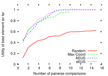
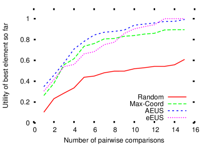
$d=10$	$d=20$
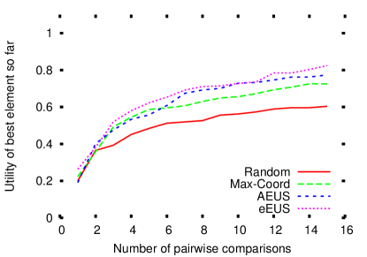
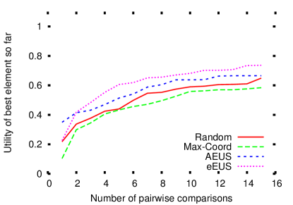
$d=50$	$d=100$

Figure 1: Performance of AEUS comparatively to baselines (see text) vs number of pairwise comparisons, depending on the dimension $d$ of the search space (results averaged over 101 runs).

The artificial active ranking problem used to investigate AEUS robustness is inspired from the active learning frame studied by [8], varying the dimension $d$ of the space in 10, 20, 50, 100 (Fig. 1).

In each run, a target utility function is set as a vector w^∗ uniformly selected in the $d$-dimensional $L_{2}$ unit sphere. A fixed sample $S=\{\mbox{\bf u}_{1},\ldots\mbox{\bf u}_{1000}\}$ of 1,000 points uniformly generated in the $d$-dimensional $L_{1}$ unit sphere is built. At iteration $t$, the sample u with best AEUS is selected in $S$; the expert ranks it comparatively to the previous best solution u_t, yielding a new ranking constraint (e.g. $\mbox{\bf u}<\mbox{\bf u}_{t}$), and the process is iterated. The AEUS performance at iteration $t$ is computed as the scalar product of u_t and w^∗.

AEUS is compared to an empirical estimate of the expected utility of selection (baseline eEUS). In eEUS, the current best sample u in $S$ is selected from Eq. (5), computed from 10,000 points w selected in the version spaces W${}_{t}^{+}$ and W${}_{t}^{-}$ and $\mbox{\bf u}_{t}$ is built as above. Another two baselines are considered: Random, where sample u is uniformly selected in $S$, and Max-Coord, selecting with no replacement u in $S$ with maximal $L_{\infty}$ norm. The Max-Coord baseline was found to perform surprisingly well in the early active ranking stages, especially for small dimensions $d$. The empirical results reported in Fig. 1 show that AEUS is a good active ranking criterion, yielding a good approximation of EUS. The approximation degrades gracefully as dimension $d$ increases: as noted by [14], the center of the largest ball in a convex set yields a lesser good approximation of the center of mass thereof as dimension $d$ increases. In the meanwhile, the approximation of the center of mass degrades too as a fixed number of 10,000 points are used to estimate EUS regardless of dimension $d$. Random selection catches up as $d$ increases; quite the contrary, Max-Coord becomes worse as $d$ increases.

4.2 Validation of April

The main goal of the experiments is to comparatively assess April with respect to inverse reinforcement learning (IRL [1], section 2). Both IRL and April extract the sought policy through an iterative two-step processes. The difference is that IRL is initially provided with an expert trajectory, whereas April receives one bit of information from the expert on each trajectory it demonstrates (its ranking w.r.t. the previous best trajectory). April performance is thus measured in terms of “expert sample complexity”, i.e. the number of bits of information needed to catch up compared to IRL. April is also assessed and compared to the black-box CMA-ES optimization algorithm, used with default parameters [12].

All three IRL, April and CMA-ES algorithms are empirically evaluated on two RL benchmark problems, the well-known mountain car problem and the cancer treatment problem first introduced by [32]. None of these problems has a reward function.

Policies are implemented as 1-hidden layer neural nets with 2 input nodes and 1 output node, respectively the acceleration for the mountain car (resp. the dosage for the cancer treatment problem). The hidden layer contains 9 neurons for the mountain car (respectively 99 nodes for the cancer problem), thus the dimension of the parametric search space is ${37}$ (resp. $397$).

RankSVM is used as learning-to-rank algorithm [16], with linear kernel and $C=100$. All reported results are averaged out of 101 independent runs.

4.2.1 The cancer treatment problem.

In the cancer treatment problem, a stochastic transition function is provided, yielding the next patient state from its current state (tumor size $s_{t}$ and toxicity level $t_{t}$) and the selected action (drug dosage level $a_{t}$):

$$\begin{array}[]{ll}s_{t+1}&=s_{t}+0.15\max(t_{t},t_{0})-1.2(a_{t}-0.5)\times 1(s_{t}>0)+\varepsilon\\ t_{t+1}&=t_{t}+0.1\max(s_{t},s_{0})+1.2(a_{t}-0.5)+\varepsilon\end{array}$$

Further, the transition model involves a stochastic death mechanism (modelling the possible patient death by means of a hazard rate model). The same setting as in [6] is considered with three differences. Firstly, we considered a continuous action space (the dosage level is a real value in $[0,1]$), whereas the action space contains 4 discrete actions in [6]. Secondly the time horizon is set to 12 instead of 6. Thirdly, a Gaussian noise $\epsilon$ with mean 0 and standard deviation $\sigma$ (ranging in 0, 0.05, 0.1, 0.2) is introduced in the transition model. The AEUS of the candidate policies is computed as their empirical AEUS average over 11 trajectories (Eq. 6).

The initial state is set to 1.3 tumor size and 0 toxicity. For the sake of reproducibility the expert preferences are emulated by favoring the trajectory with minimal sum of the tumor size and toxicity level at the end of the 12-months treatment.

The average performance (sum of tumor size and toxicity level) of the best policy found in each iteration is reported in Fig. 2. It turns out that the cancer treatment problem is an easy problem for IRL, that finds the optimal policy in the second iteration. A tentative interpretation for this fact is that the target behavior extensively visits the state with zero toxicity and zero tumor size; the learned w thus associates a maximal weight to this state. In subsequent iterations, IRL thus favors policies reaching this state as soon as possible. April catches up after 15 iterations, whereas CMA-ES remains consistently far from reaching the target policy in the considered number of iterations when there is no noise, and yields bad results (not visible on the plot) for higher noise levels.

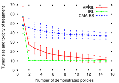
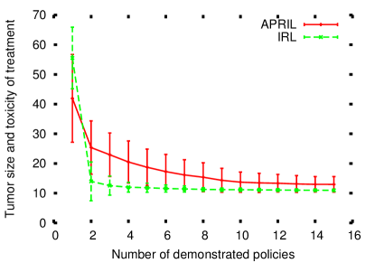
$\sigma_{noise}=0$	$\sigma_{noise}=0.05$
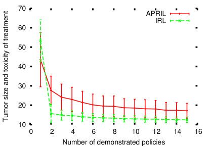
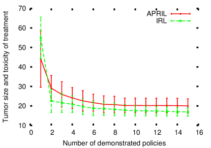
$\sigma_{noise}=0.1$	$\sigma_{noise}=0.2$

Figure 2: The cancer treatment problem: Average performance (cumulative toxicity level and tumor size after 12-months treatment) of April, IRL and CMA-ES versus the number of trajectories demonstrated to the expert, for noise level 0, .05, .1 and .2. Results are averaged over 101 runs.

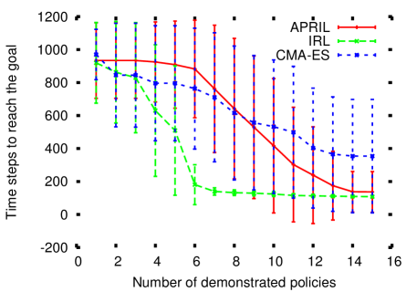
Figure 3: The mountain car problem: Average performance (number of time steps needed to reach the top of the mountain) of April, IRL and CMA-ES versus the number of trajectories demonstrated to the expert. Results are averaged over 101 runs.

4.2.2 The mountain car.

The same setting as in [31] is considered. The car state is described from its position and speed, initially set to position $-0.5$ with speed $0$. The action space is set to $\{-1,0,1\}$, setting the car acceleration. For the sake of reproducibility the expert preferences are emulated by favoring the trajectory which soonest reaches the top of the mountain, or is closest to the top of the mountain at some point during the 1000 time-step trajectory.

Interestingly, the mountain car problem appears to be more difficult for IRL than the cancer treatment problem (Fig.3), which is blamed on the lack of expert features. As the trajectory is stopped when reaching the top of the mountain and this state does not appear in the trajectory description, the target reward would have negative weights on every (other) sms feature. IRL thus finds an optimal policy after 7 iterations on average. As for the cancer treatment problem, April catches up after 15 iterations, while the stochastic optimization never catches up in the considered number of iterations.

5 Discussion and Perspectives

The Active Preference-based Reinforcement Learning algorithm presented in this paper combines Preference-based Policy Learning [2] with an active ranking mechanism aimed at decreasing the number of comparison requests to the expert, needed to yield a satisfactory policy.

The lesson learned from the experimental validation of April is that a very limited external information might be sufficient to enable reinforcement learning: while mainstream RL requires a numerical reward to be associated to each state, while inverse reinforcement learning [1, 18] requires the expert to demonstrate a sufficiently good policy, April requires a couple dozen bits of information (this trajectory improves/does not improve on the former best one) to reach state of the art results.

The proposed active ranking mechanism, inspired from recent advances in the domain of preference elicitation [29], is an approximation of the Bayesian expected utility of selection criterion; on the positive side, AEUS is tractable in high-dimensional continuous search spaces; on the negative side, it lacks the approximate optimality guarantees of EUS.

A first research perspective concerns the theoretical analysis of the April algorithm, specifically its convergence and robustness w.r.t. the ranking noise, and the approximation quality of the AEUS criterion. In particular, the computational effort of AEUS could be reduced with no performance loss by using Berstein races to decrease the number of empirical estimates (considered trajectories in Eq. 6) and confidently discard unpromising solutions [13].

Another research perspective is related to a more involved analysis of the expert’s preferences. Typically, the expert might (dis)like a trajectory because of some fragments of it (as opposed to, the whole of it). Along this line, a multiple-instance ranking setting [3] could be used to learn preferences at the fragment (sub-behavior) level, thus making steps toward the definition of sub-behaviors and modular RL.

Another further work will be concerned with hybrid policies, combining the (NN-based) parametric policy and the model of the expert’s preferences. The idea behind such hybrid policies is to provide the agent with both reactive and deliberative skills: while the action selection is achieved by the parametric policy by default, the expert’s preferences might be exploited to reconsider these actions in some (discretized) sensori-motor states.

On the applicative side, April will be experimented on large-scale robotic problems, where designing good reward functions is notoriously difficult.

Acknowledgments. The first author is funded by FP7 European Project Symbrion, FET IP 216342, http://symbrion.eu/. This work is also partly funded by ANR Franco-Japanese project Sydinmalas ANR-08-BLAN-0178-01.

References

- [1] Abbeel, P., Ng, A.: Apprenticeship learning via inverse reinforcement learning. In: Brodley, C.E. (ed.) ICML. ACM International Conference Proceeding Series, vol. 69. ACM (2004)
- [2] Akrour, R., Schoenauer, M., Sebag, M.: Preference-based policy learning. In: Gunopulos et al. [10], pp. 12–27
- [3] Bergeron, C., Zaretzki, J., Breneman, C.M., Bennett, K.P.: Multiple instance ranking. In: ICML. pp. 48–55 (2008)
- [4] Brochu, E., de Freitas, N., Ghosh, A.: Active preference learning with discrete choice data. In: Advances in Neural Information Processing Systems 20. pp. 409–416 (2008)
- [5] Calinon, S., Guenter, F., Billard, A.: On Learning, Representing and Generalizing a Task in a Humanoid Robot. IEEE transactions on systems, man and cybernetics, Part B. Special issue on robot learning by observation, demonstration and imitation 37(2), 286–298 (2007)
- [6] Cheng, W., Fürnkranz, J., Hüllermeier, E., Park, S.H.: Preference-based policy iteration: Leveraging preference learning for reinforcement learning. In: Gunopulos et al. [10], pp. 312–327
- [7] Cortes, C., Vapnik, V.: Support-vector networks. Machine Learning 20(3), 273–297 (1995)
- [8] Dasgupta, S.: Coarse sample complexity bounds for active learning. In: Advances in Neural Information Processing Systems 18 (2005)
- [9] Duda, R., Hart, P.: Pattern Classification and scene analysis. John Wiley and sons, Menlo Park, CA (1973)
- [10] Gunopulos, D., Hofmann, T., Malerba, D., Vazirgiannis, M. (eds.): Proc. European Conf. on Machine Learning and Knowledge Discovery in Databases, ECML PKDD, Part I. LNCS 6911, Springer Verlag (2011)
- [11] Hachiya, H., Sugiyama, M.: Feature selection for reinforcement learning: Evaluating implicit state-reward dependency via conditional mutual information. In: Proc. ECML/PKDD (1). Lecture Notes in Computer Science, vol. 6321, pp. 474–489 (2010)
- [12] Hansen, N., Ostermeier, A.: Completely derandomized self-adaptation in evolution strategies. Evolutionary Computation 9(2), 159–195 (2001)
- [13] Heidrich-Meisner, V., Igel, C.: Hoeffding and bernstein races for selecting policies in evolutionary direct policy search. In: ICML. p. 51 (2009)
- [14] Herbrich, R., Graepel, T., Campbell, C.: Bayes point machines. Journal of Machine Learning Research 1, 245–279 (2001)
- [15] Joachims, T.: A support vector method for multivariate performance measures. In: Raedt, L.D., Wrobel, S. (eds.) ICML. pp. 377–384 (2005)
- [16] Joachims, T.: Training linear svms in linear time. In: Eliassi-Rad, T., Ungar, L.H., Craven, M., Gunopulos, D. (eds.) KDD. pp. 217–226. ACM (2006)
- [17] Jones, D., Schonlau, M., Welch, W.: Efficient global optimization of expensive black-box functions. Journal of Global Optimization 13(4), 455–492 (1998)
- [18] Kolter, J.Z., Abbeel, P., Ng, A.Y.: Hierarchical apprenticeship learning with application to quadruped locomotion. In: NIPS. MIT Press (2007)
- [19] Konidaris, G., Kuindersma, S., Barto, A., Grupen, R.: Constructing skill trees for reinforcement learning agents from demonstration trajectories. In: Advances in Neural Information Processing Systems 23. pp. 1162–1170 (2010)
- [20] Lagoudakis, M., Parr, R.: Least-squares policy iteration. Journal of Machine Learning Research (JMLR) 4, 1107–1149 (2003)
- [21] Littman, M.L., Sutton, R.S., Singh, S.: Predictive representations of state. In: Neural Information Processing Systems 14. p. 1555–1561 (2002)
- [22] Liu, C., Chen, Q., Wang, D.: Locomotion control of quadruped robots based on cpg-inspired workspace trajectory generation. In: Proc. ICRA. pp. 1250–1255. IEEE (2011)
- [23] Ng, A., Russell, S.: Algorithms for inverse reinforcement learning. In: Langley, P. (ed.) Proc. of the Seventeenth International Conference on Machine Learning (ICML-00). pp. 663–670. Morgan Kaufmann (2000)
- [24] O’Regan, J., Noë, A.: A sensorimotor account of vision and visual consciousness. Behavioral and Brain Sciences 24, 939–973 (2001)
- [25] Peters, J., Schaal, S.: Reinforcement learning of motor skills with policy gradients. Neural Networks 21(4), 682–697 (2008)
- [26] Sutton, R., Barto, A.: Reinforcement Learning: An Introduction. MIT Press, Cambridge (1998)
- [27] Szepesvári, C.: Algorithms for Reinforcement Learning. Morgan & Claypool (2010)
- [28] Tsochantaridis, I., Joachims, T., Hofmann, T., Altun, Y.: Large margin methods for structured and interdependent output variables. Journal of Machine Learning Research 6, 1453–1484 (2005)
- [29] Viappiani, P.: Monte-Carlo methods for preference learning. In: Hamadi, Y., Schoenauer, M. (eds.) Proc. Learning and Intelligent OptimizatioN, LION 6. LNCS, Springer Verlag (2012), to appear
- [30] Viappiani, P., Boutilier, C.: Optimal Bayesian recommendation sets and myopically optimal choice query sets. In: NIPS. pp. 2352–2360 (2010)
- [31] Whiteson, S., Taylor, M.E., Stone, P.: Critical factors in the empirical performance of temporal difference and evolutionary methods for reinforcement learning. Journal of Autonomous Agents and Multi-Agent Systems 21(1), 1–27 (2010)
- [32] Zhao, Kosorok, M.R., Zeng, D.: Reinforcement learning design for cancer clinical trials. Stat Med (Sep 2009)