Identifying the Radio Bubble Nature of the Microwave Haze

Abstract

Using 7-year data from the Wilkinson Microwave Anisotropy Probe I identify a sharp “edge” in the microwave haze at high Galactic latitude ($35^{\circ}<|b|<55^{\circ}$) that is spatially coincident with the edge of the “Fermi Haze/Bubbles”. This finding proves conclusively that the edge in the gamma-rays is real (and not a processing artifact), demonstrates explicitly that the microwave haze and the gamma-ray bubbles are indeed the same structure observed at multiple wavelengths, and strongly supports the interpretation of the microwave haze as a separate component of Galactic synchrotron (likely generated by a transient event) as opposed to a simple variation of the spectral index of disk synchrotron. In addition, combining these data sets allows for the first determination of the magnetic field within a radio bubble using microwaves and gamma-rays by taking advantage of the fact that the inverse Compton gamma-rays are primarily generated by scattering of CMB photons at these latitudes, thus minimizing uncertainty in the target radiation field. Assuming uniform volume emissivity, I find that the magnetic field within our Galactic microwave/gamma-ray bubbles is $\sim 5$ $\mu$G above 6 kpc off of the Galactic plane.

1. Introduction

Recent full sky data sets by the Wilkinson Microwave Anisotropy Probe (WMAP) and the Fermi Gamma-Ray Space Telescope have revealed the presence of a new and very large structure in the Milky Way. This emission manifests as an excess of both microwaves and gamma-rays when removing Galactic diffuse emission associated with known emission mechanisms at these wavelengths and has come to be named the “WMAP Haze” (Finkbeiner, 2004; Dobler & Finkbeiner, 2008; Dobler, 2012) and the “Fermi Haze/Bubbles” (Dobler et al., 2010; Su et al., 2010) in the microwaves and gamma-rays respectively.

In microwaves, the haze is synchrotron emission with a brightness temperature as a function of frequency $T\propto\nu^{\beta_{H}}$ with $\beta_{H}\approx-2.5$ (Dobler, 2012). This spectral dependence implies that the underlying electron spectrum (number density as a function of energy) is given by $dN/dE\propto E^{\gamma}$ with $\gamma\approx-2$ for energies $\sim$10 GeV. In gamma-rays, the haze/bubbles is most likely due to inverse Compton (IC) scattering of the starlight, infrared, and cosmic microwave background (CMB) interstellar radiation field (ISRF). In the original discovery paper of the Fermi haze/bubbles, Dobler et al. (2010) showed that the spectrum of the gamma-rays is consistent with IC emission from the same electron population responsible for the microwave haze synchrotron in both energy dependence as well as overall normalization. However, as shown by Dobler (2012), the existence of $\sim$1-10 GeV IC gamma-rays at high latitude where the ISRF is dominated by the CMB require electrons with energies $\sim$TeV.

Taken together, the microwaves and gammas imply that the electron spectrum is roughly a powerlaw from $\sim$1-1000 GeV suggesting that either the electrons have not had sufficient time to cool (the cooling time in this energy range is $\sim 10^{6}$-$10^{7}$ yr; see Su et al., 2010) or are continuously being accelerated within the haze/bubbles (e.g., Dobler et al., 2011; Mertsch & Sarkar, 2011). The large volume of hard spectrum cosmic-rays has made it difficult to identify an underlying origin for the haze/bubbles and there have been numerous studies exploring the possibilities from starbursts (Biermann et al., 2010), to Galactic winds (Crocker & Aharonian, 2011), to jet blown bubbles (Guo & Mathews, 2011; Guo et al., 2011), and even co-annihilation of dark matter particles in the Galactic halo (Dobler et al., 2011).

The goal of this letter is not to delve into the origin question any further, but rather to address one of the main discrepancies between the microwave and gamma-ray haze/bubbles; namely, the observation that (as pointed out by Su et al., 2010), the gamma-ray emission appears to have a sharp edge at latitudes $|b|\approx 50^{\circ}$, while the microwaves fall off in intensity closer to $|b|\approx 35^{\circ}$ (see Dobler, 2012). In §2 I describe the component separation methods used to uncover both the microwave and gamma-ray haze/bubbles in WMAP and Fermi data, and in §3 I will show that, in fact, the microwaves also have a sharp edge at $b\approx-50^{\circ}$ that is spatially coincident with the edge in the Fermi emission. In §4 I summarize this work and describe the important implications for this microwave edge on the interpretation of the Galactic haze/bubbles.

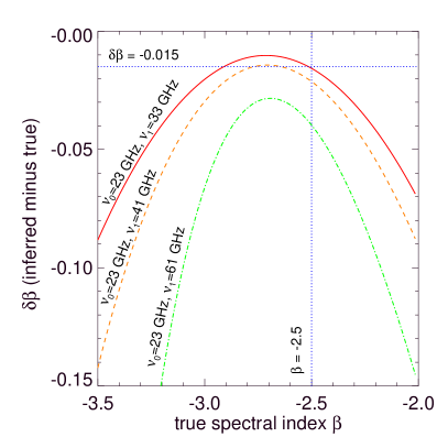
Figure 1.— The difference between the inferred and true spectral index as a function of the true index for the CMB estimate used in this letter. The inferred haze spectrum measured by Dobler & Finkbeiner (2008) and Dobler (2012) is $\beta_{H}\approx-2.55$. Since the CMB bias for a $T\propto\nu^{\beta}$ foreground with $\beta\approx-2.5$ is only 0.015, the measured spectrum is not significantly biased. This implies that the electron population has an energy distribution of $dN/dE\propto E^{-2.1}$ at $E\sim 10$ GeV.

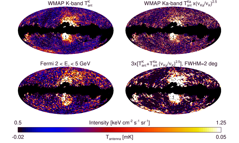
Figure 2.— Top row: the microwave haze at WMAP K- and Ka-band smoothed to $1^{\circ}$. As noted in Dobler (2012), the microwaves seem to fade quickly below $b\approx-35^{\circ}$ in contrast to the Fermi haze/bubbles (lower left) which continue down to $b\approx-50^{\circ}$. The Fermi residual is just the difference between the data and the Fermi diffuse model for visualization (see §2). However, when smoothing the WMAP data to $2^{\circ}$ and stacking with weights given by $(\nu/\nu_{\rm K})^{2.5}$ it can be seen in the lower right panel that there is an edge in the microwaves at $b\approx-50^{\circ}$ as well.

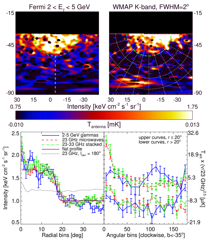
Figure 3.— Top left: the southern Fermi bubble at latitudes $b<-35^{\circ}$ where the edges are most discernible in the gammas. Top right: the same region but for the WMAP K-band haze/bubbles smoothed to $2^{\circ}$. There is a clear spatial correspondence between the Fermi haze/bubbles and the WMAP haze, including an edge at high latitudes. Taking the center of the emission to be $(\ell,b)_{\rm cen}=(-4.5^{\circ},-35.0^{\circ})$ (dashed white line) and plotting the intensity of the gammas and microwaves as a function of distance from the center (i.e., integrating over the angular bins shown in dotted lines in the upper right panel) reveals an unambiguous detection of an edge at high latitudes that is spatially coincident with the edge in the Fermi haze/bubbles as shown in the bottom left panel. This emission is well fit by a flat brightness profile with a sharp edge at $r\sim 17^{\circ}$ from the center (performing the same annular bin using $\ell_{\rm cen}=180^{\circ}$ yields no such feature). Lower right: the same but integrating over radial bins (for two ranges in $r$) as a function of angular bin.

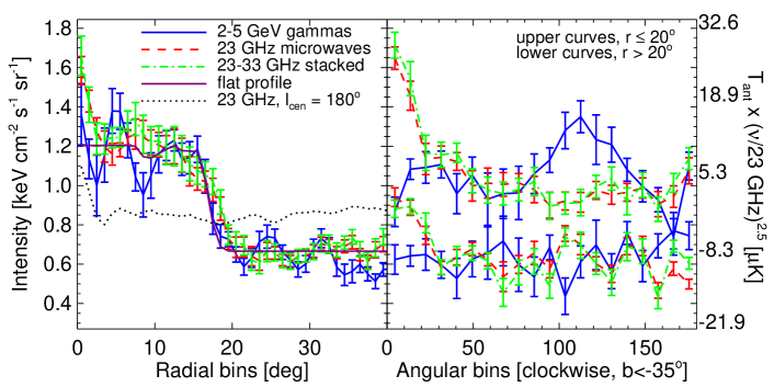
Figure 4.— The same as the bottom panels of Figure 3, but using the Fermi diffuse model in the template fit.

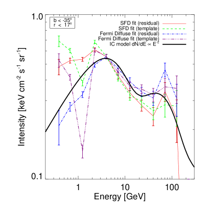
Figure 5.— The spectrum of the Fermi haze/bubble for $b<-35^{\circ}$ and within $r<17^{\circ}$ of $(\ell,b)=(-4.5^{\circ},-35^{\circ})$. The four different lines represent spectra derived from haze template or residual amplitudes for both SFD and Fermi diffuse model fits. The spectra have been normalized to the SFD residual spectrum at 4 GeV. While the uncertainty at low energies is large, the four spectral estimates agree above 4 GeV and are consistent with IC emission from an electron population with $dN/dE\propto E^{-2}$. The spectrum is softer than at lower latitudes (suggesting that the IC signal is due primarily to CMB scattering at distances $>6$ kpc above the Galactic plane), which argues for a leptonic (IC) rather than hadronic ($\pi^{0}$ decay) origin.

2. Methods

The most straightforward method for uncovering the Galactic haze/bubbles in both the WMAP and Fermi maps is via “template fitting” which uses maps at other wavelengths to morphologically trace known emission mechanisms in the data. A simple linear regression of these templates (using an appropriate mask) against the data yields template amplitudes which can be used to “peel away” these foregrounds. In this letter, the templates are fit at each frequency (energy) for the WMAP (Fermi) data implying that no constraint is put on the shape of the spectrum of each emission mechanism, though it is assumed that the spectrum does not vary significantly with position. The details of the template fitting used here can be found in Dobler & Finkbeiner (2008) and Dobler (2012) (hereafter DF08 and D12 respectively) for the microwaves and Dobler et al. (2010) for the gammas.

2.1. WMAP analysis

For the WMAP analysis, the templates used are the Schlegel et al. (1998) (SFD) dust map evaluated at 94 GHz by Finkbeiner et al. (1999) (FDS), the Haslam et al. (1982) 408 MHz map, and the Finkbeiner (2003) H$\alpha$ composite map. These templates are meant to trace the three primary Galactic emission mechanisms at microwave wavelengths: thermal and spinning dust (FDS), soft synchrotron (Haslam), and free–free (H$\alpha$). In addition, I include the haze and hard disk bivariate Gaussian templates used in D12. Because the CMB is of comparable brightness to the haze at WMAP wavelengths, I presubtract the CMB5 estimate for the haze given by DF08. Pixels for which the dust extinction at H$\alpha$ is greater than 1 magnitude and for which the H$\alpha$ intensity is greater than 10 Rayleigh are masked in the fit, as well all point sources in the WMAP and Planck ERCSC (30 GHz to 143 GHz) catalogs.

These Galactic templates are fit to the WMAP data via the regression equation ${\bf w}_{\nu}-{\bf c}={\bf P}\vec{a}_{\nu}$ where ${\bf w}_{\nu}$ is a map of the WMAP data at frequency $\nu$, ${\bf c}$ is the CMB5 estimate, and ${\bf P}$ is a matrix of template maps. The equation is solved for the coefficients $\vec{a}_{\nu}=({\bf P}^{\rm T}{\bf n}_{\nu}^{-1}{\bf P})^{-1}({\bf P}^{\rm T}{\bf n}_{\nu}^{-1})({\bf w}_{\nu}-{\bf c})$ where ${\bf n}$ is the mean noise in a given band. The haze residual in each band is defined as $R_{H}\equiv{\bf w}_{\nu}-{\bf c}-{\bf P}\vec{a}_{\nu}+a^{H}_{\nu}\times H$ where $H$ is the haze template. That is, it is the residual of the regression plus the amount of haze template removed. In order to account for spectral variations with position, the fit is performed independently on the regions given in D12. A composite $R_{H}$ is constructed from the union of those regions.

2.2. Fermi analysis

At Fermi energies, there are three main sources of diffuse gamma-ray emission from the Galaxy: bremsstrahlung, IC, and $\pi^{0}$ decay. The latter component is the dominant emission mechanism at high latitudes. For the purpose of comparing the haze/bubbles in Fermi to the emission in WMAP, this letter concentrates on the extreme high Galactic southern latitudes, $b<-35^{\circ}$. High northern Galactic latitudes are contaminated by dust-correlated emission in both the microwaves (likely spinning dust; see Draine & Lazarian, 1998; Dobler et al., 2009) and the gammas ($\pi^{0}$ decay) and make a clear separation of the haze/bubbles emission difficult in both datasets.

Because the $\pi^{0}$’s are created via collisions of cosmic-ray protons with the ISM, I use the SFD map of dust column density as a template for this emission since it is a reasonable tracer of dust and gas in our Galaxy. It is important to note that this template is an integrated column density while $\pi^{0}$ emission is proportional to the ISM density times the proton number density, and so line-of-sight effects render the SFD map an imperfect tracer of $\pi^{0}$ emission. This has dramatic effects at low latitudes in the haze/bubbles regions as pointed out by Dobler et al. (2011), however for $b<-35^{\circ}$ as is used here, a simple two template (SFD plus bivariate Gaussian; see Dobler et al., 2010) description of the data is sufficient to isolate the Fermi haze/bubbles emission.

As in Dobler et al. (2010) the fit minimizes the log-likelihood, $\ln{\mathcal{L}}=\sum_{i}[k_{i}\ln\mu_{i}-\mu_{i}-\ln(k_{i}!)]$, where $k_{i}$ is the map of observed counts at pixel $i$, $\mu$ is a synthetic counts map given by $\mu(E)=S(E)\times({\rm mask})\times({\rm exposure})$, and $S(E)$ is the synthetic sky map $S(E)=b_{\rm SFD}\times{\rm SFD}+b_{H}\times H+b_{\rm uni}$. This log-likelihood is minimized over the template amplitudes $b_{\rm SFD}$, $b_{H}$, and $b_{\rm uni}$ (a spatially uniform contribution) for pixels outside of the mask and for $b<-35^{\circ}$. I emphasize that this is not meant to represent a perfect model for the diffuse emission from our Galaxy, but rather serves to effectively isolate the Fermi haze/bubbles emission so that it can be morphologically compared to the microwave emission. For a thorough analysis of Galactic diffuse emission observed by Fermi see The Fermi-LAT Collaboration (2012). Lastly, the analysis was also redone using the Fermi diffuse model (gll_iem_v02.fit) as opposed to the SFD map as a template and the results are not significantly changed.

3. Results

Directly comparing the haze/bubbles residuals at high latitude will involve weighted stacking of $R_{H}$ in multiple WMAP bands, and so it is useful to estimate the extent to which the spectrum of the microwave emission is affected by the CMB bias described in DF08. This bias comes from the fact that any CMB estimate used in §2 will inherently have some residual foregrounds after cleaning emission from the Galaxy, and since that CMB estimate is presubtracted with a fixed CMB spectrum, this imprints a bias on the inferred haze spectrum (see DF08). The CMB estimate used here is generated by the linear combination of the WMAP data that minimizes the variance in unmasked pixels of ${\bf c}=\sum_{j}\zeta_{j}{\bf w}_{j}^{\prime}$ where ${\bf w}_{j}^{\prime}$ is the WMAP data minus the FDS prediction for thermal dust emission in each band $j$ and $\sum_{j}\zeta_{j}\equiv 1$ for ${\bf w}$ in thermodynamic $\Delta T$ units.

This last constraint on $\zeta$ has the consequence that the measured spectrum cannot be used to infer the true spectrum. That is, while the amplitude of the bias can be estimated as in DF08, the exact bias cannot be known. However, it is possible to answer the question: for a foreground with a given true spectrum $T_{\rm antenna}\propto\nu^{\beta_{\rm true}}$, what would be the inferred spectral index $\beta_{\rm infer}$? This $\delta\beta\equiv\beta_{\rm infer}-\beta_{\rm true}$ is shown as a function of $\beta_{\rm true}$ in Figure 1. Despite the very large possible CMB bias, for a true spectral index of $\beta_{\rm true}=-2.5$, the inferred spectral index when comparing K- to Ka-band would only be biased by $\delta\beta=-0.015$ given the CMB5 coefficients $\zeta=(0.11,-0.48,0.12,0.16,1.09)$. The implication is that the spectrum measured by DF08 and D12 for the microwave haze $T_{H}\propto\nu^{\beta_{H}}$ with $\beta_{H}\approx-2.5$ is likely not significantly biased and the underlying electron population is very close to $dN/dE\propto E^{-2}$.

The full sky residuals $R_{H}^{W}$ and $R_{H}^{F}$ — the haze/bubbles in WMAP and Fermi data — are shown in Figure 2 and illustrate several of the key characteristics noted in previous studies: scaling $R_{H}^{W}$ by $\nu^{2.5}$ yields roughly equal brightness indicating a $T\propto\nu^{-2.5}$ spectrum (Dobler & Finkbeiner, 2008), $R_{H}^{W}$ and $R_{H}^{F}$ are roughly spatially coincident at low latitudes (Dobler et al., 2010; Su et al., 2010), at $1^{\circ}$ smoothing $R_{H}^{W}$ appears to fade quickly below $b=-35^{\circ}$ (Dobler, 2012), and $R_{H}^{F}$ appears to have a sharp “edge” at $|b|\sim 50^{\circ}$ (Su et al., 2010). The lack of a similar edge in the WMAP data at $b\sim-50^{\circ}$ in WMAP has led to some ambiguity about whether the WMAP haze and the Fermi haze/bubbles are in fact the same structure. However, creating the weighted stack of the WMAP emission $R_{H}^{\rm K}+(\nu_{\rm Ka}/\nu_{\rm K})^{2.5}\times R_{H}^{\rm Ka}$ and smoothing to $2^{\circ}$ (i.e., the same smoothing as the Fermi map) reveals an edge in the microwave haze that appears coincident with the southern edge in the gamma-ray bubbles.

To assess the significance of this feature, I zoom in on the extreme southern latitudes with $b<-35^{\circ}$ in Figure 3 (corresponding to heights $>6$ kpc above the GC), and a clear sharp edge is evident in both the gamma-rays and the microwaves. As noted in Su et al. (2010) the center of the Fermi bubble at these latitudes is roughly $\ell\sim-4.5^{\circ}$. Binning the sky into polar bins centered on the bubble center $(\ell_{\rm cen},b_{\rm cen})=(-4.5^{\circ},-35^{\circ})$, integrating annuli with unmasked pixel latitudes $<-35^{\circ}$ (see figure), and plotting as a function of distance from the bubble center, the lower left panel of Figure 3 shows the southern Fermi bubble edge described in Su et al. (2010). The same plot generated with the microwaves also shows a clear edge that is spatially coincident with the Fermi bubble edge, located at roughly $r=17^{\circ}$ from the bubble center. For the $2^{\circ}$ smoothing shown here, the statistical significance of the edge identified in this way is high for both the K-band microwave haze/bubbles and the K-, Ka-band weighted stack (a null test calculated by setting $(\ell_{\rm cen},b_{\rm cen})=(-180^{\circ},-35^{\circ})$ shows no evidence for an edge at the Galactic anti-center). Finally, by integrating a uniform brightness, infinitely sharp edge (smoothed to $2^{\circ}$ and with the same mask) in the same way, Figure 3 shows that Fermi and WMAP bubbles are consistent with a sharp edge.

While this is a clear detection of an edge in the WMAP haze, there is angular dependence in the microwave emission that is not readily apparent in the gamma-rays. Figure 3 shows the emission as a function of annulus angle both inside and outside the haze/bubbles ($r<20^{\circ}$ and $r>20^{\circ}$ from $(\ell_{\rm cen},b_{\rm cen})$) in the lower right panel and indicates an “arm” of emission in the microwaves for annular angles less than $\sim 30^{\circ}$. No such arm is evident in the gamma-rays. For annular angles greater than $30^{\circ}$ there is no other clear structure present in the microwaves though the microwave bubble emission is detected in each angular bin (i.e., there is an excess of emission interior to the microwave edge compared to exterior). Figure 4 shows the same results, but using the Fermi diffuse model template in the fit. While the overall amplitude of the gamma-ray signal is slightly lower, the edge is still spatially coincidence with the edge in microwaves.

Figure 5 shows the spectrum of the Fermi haze/bubble for $b<-35^{\circ}$ and within $r<17^{\circ}$ of the bubble center for four different spectral estimates: using the SFD map or the Fermi diffuse model in the template fit and estimating the spectrum via unmasked pixels in $a_{\nu}^{H}\times H$ or $R_{H}$. Below $\sim 4$ GeV, the four different types of spectral estimates differ, indicating a systematic bias in the derived spectrum due to imperfect template approximations and/or brighter, softer components leaking into the residuals. However, above $\sim 4$ GeV, the spectra are all consistent with IC from electrons scattering predominantly off of CMB photons and having a spectrum $dN/dE\propto E^{-2}$ (i.e., the same as that required to make the $T\propto\nu^{-2.5}$ microwave haze spectrum). It is interesting to note that this spectrum of the “cap” of the bubble is somewhat softer than that found by Dobler et al. (2010) and Su et al. (2010) who include lower latitudes, in agreement with the IC scenario (since the higher energy optical and IR components of the ISRF have lower amplitude at high latitudes) and inconsistent with a hadronic scenario, which is also disfavored by the detection of the microwave haze at $b<-35^{\circ}$ in Figure 3.

Since the IC emission is a function of the number density of electrons $dN/dE$ and the ISRF intensity while the synchrotron intensity depends on $dN/dE$ and the magnetic field $B$, an estimate of $B$ can be made under several simplifying assumptions. Given the (CMB dominated) ISRF model above and assuming the same $dN/dE=N_{0}\times E^{-2}$ for both signals, a uniform magnetic field and volume emissivity model above 6 kpc ($b<-35^{\circ}$) yields $B\sim 5$ $\mu$G within the southern bubble.

4. Summary

Using 7-year WMAP data to isolate the microwave haze and comparing this to the Fermi haze/bubbles at southern Galactic latitudes less than $-35^{\circ}$, I have presented the detection of a sharp edge in the microwave haze that is coincident with the Fermi bubble edge. This microwave bubble edge is evident when smoothing the haze to 2^∘ in both the K-band WMAP data as well as a stack of K- and Ka-band weighted by $\nu^{2.5}$, where $\nu$ is the microwave band. I have also shown explicitly that, for the CMB estimate used in this study as well as Dobler (2012), the $\nu^{-2.5}$ spectrum of the microwave haze/bubbles is not significantly biased by systematics indicating that the electrons responsible for generating this synchrotron have a number density as a function of energy $dN/dE\propto E^{-2}$, in excellent agreement with the inverse Compton interpretation of the gamma-rays.

The detection of an edge in the microwave haze $\sim 50^{\circ}$ above the plane and coincident with the Fermi haze/bubbles has several important consequences. First, it proves conclusively that the microwave and and the Fermi bubbles are the same structure observed at multiple wavelengths. Second, given the vastly different experiments, the detection of an edge in microwaves proves that the edge in gammas is real and not due to processing artifacts or low photon counts in the maps generated by Dobler et al. (2010) and Su et al. (2010). Finally, the sharp edge, coupled with the hard spectrum of the emission, suggests a transient event for the origin of the microwave haze indicating that it is a separate component of diffuse emission in our Galaxy and not merely a spatial variation in the spectral index of the disk synchrotron.

Acknowledgments: I thank Peng Oh, Christoph Pfrommer, Krzysztof Gorskí, Neal Weiner, and Doug Finkbeiner for useful conversations. This work has been supported by the Harvey L. Karp Discovery Award.

References

- Biermann et al. (2010) Biermann, P. L., Becker, J. K., Caceres, G., Meli, A., Seo, E.-S., & Stanev, T. 2010, ApJ, 710, L53
- Crocker & Aharonian (2011) Crocker, R. M., & Aharonian, F. 2011, Physical Review Letters, 106, 101102
- Dobler (2012) Dobler, G. 2012, ApJ, 750, 17
- Dobler et al. (2011) Dobler, G., Cholis, I., & Weiner, N. 2011, ApJ, 741, 25
- Dobler et al. (2009) Dobler, G., Draine, B., & Finkbeiner, D. P. 2009, ApJ, 699, 1374
- Dobler & Finkbeiner (2008) Dobler, G., & Finkbeiner, D. P. 2008, ApJ, 680, 1222
- Dobler et al. (2010) Dobler, G., Finkbeiner, D. P., Cholis, I., Slatyer, T., & Weiner, N. 2010, ApJ, 717, 825
- Draine & Lazarian (1998) Draine, B. T., & Lazarian, A. 1998, ApJ, 494, L19
- Finkbeiner (2003) Finkbeiner, D. P. 2003, ApJS, 146, 407
- Finkbeiner (2004) —. 2004, ApJ, 614, 186
- Finkbeiner et al. (1999) Finkbeiner, D. P., Davis, M., & Schlegel, D. J. 1999, ApJ, 524, 867
- Guo & Mathews (2011) Guo, F., & Mathews, W. G. 2011, arXiv:1103.0055
- Guo et al. (2011) Guo, F., Mathews, W. G., Dobler, G., & Oh, S. P. 2011, arXiv:1110.0834
- Haslam et al. (1982) Haslam, C. G. T., Salter, C. J., Stoffel, H., & Wilson, W. E. 1982, A&AS, 47, 1
- Mertsch & Sarkar (2011) Mertsch, P., & Sarkar, S. 2011, Physical Review Letters, 107, 091101
- Pietrobon et al. (2011) Pietrobon, D., et al. 2011, arXiv:1110.5418
- Schlegel et al. (1998) Schlegel, D. J., Finkbeiner, D. P., & Davis, M. 1998, ApJ, 500, 525
- Su et al. (2010) Su, M., Slatyer, T. R., & Finkbeiner, D. P. 2010, ApJ, 724, 1044
- The Fermi-LAT Collaboration (2012) The Fermi-LAT Collaboration. 2012, arXiv:1202.4039