On the Efficient Calculation of a Linear Combination of Chi-Square Random Variables with an Application in Counting String Vacua

Abstract

Linear combinations of chi square random variables occur in a wide range of fields. Unfortunately, a closed, analytic expression for the pdf is not yet known. Starting out from an analytic expression for the density of the sum of two gamma variables, a computationally efficient algorithm to numerically calculate the linear combination of chi square random variables is developed. An explicit expression for the error bound is obtained. The proposed technique is shown to be computationally efficient, i.e. only polynomial in growth in the number of terms compared to the exponential growth of most other methods. It provides a vast improvement in accuracy and shows only logarithmic growth in the required precision. In addition, it is applicable to a much greater number of terms and currently the only way of computing the distribution for hundreds of terms. As an application, the exponential dependence of the eigenvalue fluctuation probability of a random matrix model for 4d supergravity with N scalar fields is found to be of the asymptotic form exp(-0.35N).

1 Review and Main Results

1.1 Introduction

Linear combinations of $\chi^{2}$ random variables occur in many different fields, in statistical hypothesis testing as well as in high energy physics. In string theory, they have had a relative recent comeback, occurring frequently in the study of random matrix models, such as the spectral analysis of the Wishart ensemble. Those models have proven an invaluable tool for making statistical claims about the existence of stable vacua in various theories of supergravity. We will revisit one of these applications in section 5.

For a full understanding of a random variable, its distribution is of course of utmost importance. Unfortunately, for the probability density function (pdf) of a linear combination of $\chi^{2}$ random variables, there is no known closed analytic expression yet. The great number of related publications—see section 1.2—proves the ongoing interest in this topic.

It is surprising, however, that none of the known methods for calculating this pdf seems computationally viable for more than a handful of terms, at most. In fact, the ones that are accurate enough suffer from exponential growth in the number of terms to calculate, see for example [2] and the comment on this method in [3]. Other known methods are discussed in section 1.2.

Unfortunately, this lack of methodology proved to be an obstacle to making quantitative analytic claims about the existence of aforementioned vacua in a model of $4d$ random supergravity, see [4]. Motivated by this fact, we present a relatively simple procedure that is nonetheless far superior in speed and accuracy to the hitherto published methods.

1.2 The Existing Literature

As already mentioned, there exist many approaches to calculating or approximating the distribution of a linear combination of $\chi^{2}$ random variables. For our purposes, one exclusion criterion is that the method has to be quantitatively accurate, which means that we need an explicit expression for the error. This excludes fits to other distributions, as for examples the three moment fit suggested by [5], or the more recent mixture approximation by [6].

Unfortunately, it also excludes saddlepoint or method of deepest descent approximations, see for example [7, Sec. 5], which involves several steps that make it hard to track the error accurately. Let us discuss the techniques which pass this requirement.

One brute-force method is of course to draw a couple of million random variables, multiply them with the weights and calculate the distribution empirically. This works well when one is interested in the quantiles that lie around the bulk of the mass. In our example, however, the very low quantiles are of interest, and we simply do not have enough statistics to calculate those. Note that importance sampling can—unfortunately—not be used, since we do not know the complete distribution.

Another often-used ansatz is to expand the moment generating function in a series representation and inverting term by term. One such example (for gamma random variables) is given in [8]. Unfortunately, the prefactors in the expansion cannot be calculated in polynomial time. Another example (for chi squares) is [9] where, again, the prefactors are hard to compute. The method targeted at exponential distributions suggested in [10] suffers from the same exponential growth, which is easy to see by looking at the suggested functional form. A more recent example is [11], which uses Laguerre polynomials. The same problem persists here; in addition, the error bound given suggests that obtaining an accurate result will require a very large number of terms.

As a third group, there are techniques that use numerical integration to obtain the density function, see for example [12] and [3]. Unfortunately, in both papers, the number of dimensions over which we have to integrate for $n$ terms is $n-1$. While this might be feasible for small $n$, it is not for our application—just sampling two points in any direction grows as $2^{n}$, and even using sophisticated Monte Carlo or Gibbs sampling algorithms does not help when $n$ is of order $1000$. Another method, which has only one integral to calculate, [13], has the problem of a highly oscillatory integrand that has to be integrated over $\mathds{R}$, which seems impossible to do to the required accuracy.

To summarize, none of the above-mentioned techniques is feasible in our regime of interest—either due to computational restrictions or because the answer is not precise enough. It should be noted, however, that calculating exponentially small derivations is not something one normally encounters in statistics, so it comes as no surprise that methods for that regime are yet to be developed. In this paper, we develop a method which is both fast, arbitrarily accurate and computationally efficient even for a vast number of terms, especially in the low quantile regime that we are interested in.

2 Analytic Results

2.1 Main Result

We will first state the main result and prove the details in due course.

As stated in the first chapter, the problem is to calculate the density function of $Z=\sum_{i=1}^{n}a_{i}X_{i}$, where $X_{i}\sim\chi^{2}_{r}$ are iid random variables for some $r>0$ and $a_{i}\in\mathds{R}_{>0}$. Let $\mathbf{T}_{n}:\mathcal{C}^{n}\rightarrow\mathds{R}[n]$ denote the Taylor-Maclaurin map which assigns to a function its Taylor polynomial to order $n$ around $0$, and $\mathbf{R}_{n}:\mathcal{C}^{n}\rightarrow\mathcal{C}^{n}$ its associated remainder map.

Theorem 1.

Let $r\in 2\mathds{N}_{0}+1$, $Z=\sum_{i=1}^{n}\left(a_{i}X_{i}+b_{i}Y_{i}\right)$, $X_{i},Y_{j}\sim\chi^{2}_{r}$ iid random variables, $a_{i},b_{i}\in\mathds{R}_{>0}$ for some $n>0$ and $a_{1}<b_{1}<...<a_{n}<b_{n}$. Let $m_{1},...,m_{n}\in\mathds{N}_{0}$ and $\bar{m}:=\max\{m_{1},...,m_{n}\}$. Then the density function $f_{Z}$ is given by

$$f_{Z}(x)=C\theta(x)\left(\mathrm{T}(x)+\mathrm{R}(x)\right)\quad,$$

where ${{}{}{}{}{}{}{}{}{}{}}{{}{}{}{}{}{}{}{}{}{}}\raisebox{-3.6pt}{\leavevmode\resizebox{11.99998pt}{}{$*$}}_{i=1}^{n}f_{i}:=f_{1}\bar{*}...\bar{*}f_{n}$,

$$\mathrm{T}(x)=\left(\overset{n}{\underset{i=1}{{{}{}{}{}{}{}{}{}{}{}}{{}{}{}{}{}{}{}{}{}{}}\raisebox{-5.80002pt}{\leavevmode\resizebox{16.00008pt}{}{$*$}}}}\mathrm{e}^{-\frac{a_{i}+b_{i}}{4a_{i}b_{i}}\cdot}\left(\mathbf{T}_{m_{i}}\mathrm{I}_{\frac{r}{2}-\frac{1}{2}}\right)\left(\frac{b_{i}-a_{i}}{4a_{i}b_{i}}\cdot\right)\right)(x)$$

and

$$C=\left(\frac{\Gamma\left(\frac{1}{2}-\frac{r}{2}\right)}{\Gamma(r)}\right)^{\!\!\!n}\prod_{i=1}^{n}(4a_{i}b_{i})^{-r}\left(\frac{b_{i}-a_{i}}{8a_{i}b_{i}}\right)^{\!\frac{1}{2}-\frac{r}{2}}$$

and

$$0<\mathrm{R}(x)< \ \bar{\mathrm{R}}(x)-\mathrm{T}(X)$$

$$:=\left(\overset{n}{\underset{i=1}{{{}{}{}{}{}{}{}{}{}{}}{{}{}{}{}{}{}{}{}{}{}}\raisebox{-5.80002pt}{\leavevmode\resizebox{16.00008pt}{}{$*$}}}}\mathrm{e}^{-\frac{a_{i}+b_{i}}{4a_{i}b_{i}}\cdot}\left(\mathbf{T}_{m_{i}}\mathrm{I}_{\frac{r}{2}-\frac{1}{2}}+\mathrm{R}_{i}\right)\left(\frac{b_{i}-a_{i}}{4a_{i}b_{i}}\cdot\right)\right)(x)-\mathrm{T}(x)\quad.$$

Finally, $\forall x\leq y\in\mathds{R}_{>0}$, $\mathrm{R}_{i}$ is bounded by

$$\mathrm{R}_{i}(x) :=\mathbf{R}_{m_{i}}\mathrm{I}_{\frac{r}{2}-\frac{1}{2}}\left(\frac{b_{i}-a_{i}}{4a_{i}b_{i}}x\right)$$

$$\leq\frac{x^{m_{i}+1}}{(m_{i}+1)!}\ \left(\frac{b_{i}-a_{i}}{4a_{i}b_{i}}\right)^{m_{i}+1}\mathrm{I}_{\frac{r}{2}-\frac{1}{2}}^{(m_{i}+1)}\left(\frac{b_{i}-a_{i}}{4a_{i}b_{i}}y\right)\quad.$$

This result—simple as it is—does not look particularly promising, since it contains a convolution of exponentially many terms. Fortunately, though, the next statement shows that this method is indeed surprisingly easy to compute, at least for $r=1$.

Theorem 2.

Let the setup be as in theorem 1. Then the computational complexity to calculate a value $x$ of $f_{Z}$ with relative error smaller than $R_{\mathrm{max}}\in(0,1)$ is $\mathrm{O}(n^{2}r^{2}\bar{y}^{2}(\log rn-\log(R_{\mathrm{max}})))$, where $\bar{y}:=x\max_{i=1,...,n}\{\frac{b_{i}-a_{i}}{4b_{i}a_{i}}\}$.

In other words, this means that the algorithm is at most polynomial in the number of terms in our sum, polynomial in the degrees of freedom, polynomial in $\bar{y}$ as given above and logarithmically in the precision we want to obtain.

Our numerical analysis shows that this bound is by no means optimal.

We will now give a rather detailed proof. The mathematics involved is not particularly deep, but contains some ideas that are essential for later use.

2.2 The Linear Combination of Two Gamma and $\chi^{2}$ Random Variables

Definition 1.

Let $X\sim\Gamma(\alpha,\beta)$ be a gamma-distributed random variable with shape parameter $\alpha\in\mathds{R}_{>0}$ and rate parameter $\beta\in\mathds{R}_{>0}$. Then its density function $f_{X}$ is given by

$$f_{X}(x)=\theta(x)\frac{\beta^{\alpha}}{\Gamma(\alpha)}x^{\alpha-1}e^{-\beta x}\quad.$$ (1)

Note the following

Remark 1.

If $X\sim\Gamma(\alpha,\beta)$, then $cX\sim\Gamma(\alpha,c\beta)$ for $c\in\mathds{R}_{>0}$.

This is why $\beta$ is also called inverse shape parameter. This immediately leads me to the following

Lemma 1.

Let $Z=X+Y$ where $X\sim\Gamma(\alpha_{1},\beta_{1})$ and $Y\sim\Gamma(\alpha_{2},\beta_{2})$ are independent Gamma distributions. Then the density function $f_{Y}$ is given by

$$f_{Z}(z)=\theta(z)\frac{\beta_{1}^{\alpha_{1}}\beta_{2}^{\alpha_{2}}}{\Gamma(\alpha_{1}+\alpha_{2})}z^{\alpha_{1}+\alpha_{2}-1}\mathrm{e}^{-\beta_{2}z}{{}_{1}\mathrm{F}_{1}}(\alpha_{1};\alpha_{1}+\alpha_{2};(\beta_{2}-\beta_{1})z)\quad,$$ (2)

where ${}_{1}\mathrm{F}_{1}$ is a confluent hypergeometric function (Kummers function of the first kind).

Proof.

We have to calculate the convolution $f_{Z}\equiv f_{X}*f_{Y}$ over $\mathds{R}$.

$$(f_{X} *f_{Y})(z)$$

$$=\frac{\beta_{1}^{\alpha_{1}}\beta_{2}^{\alpha_{2}}}{\Gamma(\alpha_{1})\Gamma(\alpha_{2})}\int_{\mathds{R}}\theta(x)\theta(z-x)x^{\alpha_{1}-1}(z-x)^{\alpha_{2}-1}\mathrm{e}^{-\beta_{1}x-\beta_{2}(z-x)}\mathrm{d}x$$

$$=\frac{\beta_{1}^{\alpha_{1}}\beta_{2}^{\alpha_{2}}}{\Gamma(\alpha_{1})\Gamma(\alpha_{2})}\mathrm{e}^{-\beta_{2}z}\theta(z)\int_{0}^{z}x^{\alpha_{1}-1}(z-x)^{\alpha_{2}-1}\mathrm{e}^{(\beta_{2}-\beta_{1})x}\mathrm{d}x\quad,$$

which can be further simplified by substituting $x=zt\Rightarrow\mathrm{d}x=z\mathrm{d}t$, so

$$(f {}_{X}*f_{Y})(z)$$

$$=\theta(z)\frac{\beta_{1}^{\alpha_{1}}\beta_{2}^{\alpha_{2}}}{\Gamma(\alpha_{1})\Gamma(\alpha_{2})}\mathrm{e}^{-\beta_{2}z}z^{\alpha_{1}-1+\alpha_{2}-1+1}\int_{0}^{1}t^{\alpha_{1}-1}(1-t)^{\alpha_{2}-1}\mathrm{e}^{(\beta_{2}-\beta_{1})zt}\mathrm{d}t$$

$$\equiv\theta(z)\frac{\beta_{1}^{\alpha_{1}}\beta_{2}^{\alpha_{2}}}{\Gamma(\alpha_{1})\Gamma(\alpha_{2})}\mathrm{e}^{-\beta_{2}z}z^{\alpha_{1}+\alpha_{2}-1}\frac{\Gamma(\alpha_{1})\Gamma(\alpha_{2})}{\Gamma(\alpha_{1}+\alpha_{2})}{{}_{1}\mathrm{F}_{1}}(\alpha_{1};\alpha_{1}+\alpha_{2};(\beta_{2}-\beta_{1})z)$$

$$=\theta(z)\frac{\beta_{1}^{\alpha_{1}}\beta_{2}^{\alpha_{2}}}{\Gamma(\alpha_{1}+\alpha_{2})}z^{\alpha_{1}+\alpha_{2}-1}\mathrm{e}^{-\beta_{2}z}{{}_{1}\mathrm{F}_{1}}(\alpha_{1};\alpha_{1}+\alpha_{2};(\beta_{2}-\beta_{1})z)\quad,$$

where we have used the integral representation of ${}_{1}\mathrm{F}_{1}$ in the second to last line. ∎

Observe that equation 2 is indeed symmetric under exchange of the subscripts ${}_{1}\leftrightarrow{}_{2}$, as expected.

Definition 2.

Let $X\sim\chi^{2}_{k}$ be a chi-square random variable with $k$ degrees of freedom. Then the density function $f_{X}$ is given by

$$f_{X}(x)=\theta(x)\frac{x^{\frac{k}{2}-1}e^{-\frac{x}{2}}}{2^{\frac{k}{2}}\Gamma\left(\frac{k}{2}\right)}\ \quad.$$ (3)

Remark 2.

If $X\sim\chi^{2}_{k}$, then $aX\sim\Gamma\left(\frac{k}{2},\frac{1}{2a}\right)$ for $a\in\mathds{R}_{>0}$.

As a second important result, which will find its application later, we conclude the following

Corollary 1.

Let $X,Y\sim\chi^{2}_{k}$ two iid chi-square random variables with $k$ degrees of freedom. Let $Z:=aX+bY$, $a,b\in\mathds{R}_{>0}$. Then the density function $f_{Z}$ is given by

$$f_{Z}(z)=\theta(z)\frac{1}{(4ab)^{k}}\left(\frac{a-b}{8ab}\right)^{\frac{1}{2}-\frac{k}{2}}\frac{\Gamma\left(\frac{1}{2}+\frac{k}{2}\right)}{\Gamma(k)}\ \mathrm{e}^{-\frac{a+b}{4ab}z}\ x^{\frac{k}{2}-\frac{1}{2}}\ \mathrm{I}_{\frac{k}{2}-\frac{1}{2}}\left(\frac{b-a}{4ab}z\right)\quad,$$ (4)

where $\mathrm{I}_{\nu}$ is the $\nu$th order modified Bessel function of the first kind.

Proof.

This follows from lemma 1, remark 2 and from the identity (known as Kummer’s second transform)

$${{}_{1}\mathrm{F}_{1}}(\alpha;2\alpha;x)\equiv\mathrm{e}^{\frac{x}{2}}\left(\frac{x}{4}\right)^{\frac{1}{2}-\alpha}\Gamma\left(\frac{1}{2}+\alpha\right)\mathrm{I}_{\alpha-\frac{1}{2}}\left(\frac{x}{2}\right)\quad.\qed$$

Equation 4 struck my interest for the following reason: for small $z$, given $a$ and $b$ are of the same order, the prefactor in the modified Bessel function is small, so a promising ansatz for an approximation should be a Taylor-Maclaurin series for $\mathrm{I}_{\nu}$. The exponential then restricts most of the mass to lower values of $z$, which, in addition, suppresses the error introduced from the expansion. Furthermore, the leading nontrivial expansion term of $\mathrm{I}_{0}(z)$ is of order $\mathrm{O}(z^{2})$ and for general $\mathrm{I}_{\nu}$ only every second order monomial is present. All this will be quantified in the next chapters.

At first, though, we need some more results that will come into play later.

2.3 Convolution Algebra

Definition 3.

Let $\bar{*}:\mathcal{C}(\mathds{R})\times\mathcal{C}(\mathds{R})\rightarrow\mathcal{C}(\mathds{R})$ be defined as

$$(f\ \bar{*}\ g)(z)=\int_{\mathds{R}}\theta(x)\theta(z-x)f(x)g(z-x)\mathrm{d}x\equiv\int_{0}^{z}f(x)g(z-x)\mathrm{d}x$$

for $f,g\in\mathcal{C}(\mathds{R})$.

This map is well-defined, as follows from [14], Th. 1.3, and could well be extended to spaces such as $\mathrm{L}^{1}(\mathds{R})$, but we do not need more here. Important is the following

Lemma 2.

Let $\mathrm{P}_{N}:=\{\mathrm{e}^{b_{i}x}x^{n_{i}}:b_{i}\in\mathds{R},n_{i}\in\mathds{N}_{0},n_{i}<N\}$ where $N\in\mathds{N}$. Let further $f,g\in\mathrm{P}_{N}$: $f(x)=\mathrm{e}^{ax}x^{n}$, $g(x)=\mathrm{e}^{bx}x^{m}$ and define

$$(f\ \tilde{*}\ g)(x):=\left\{\begin{array}[]{lr}0&:a=b\\ (f\ \bar{*}\ g)(x)&:a\neq b\end{array}\right.\quad.$$

Then $(\left<\mathrm{P}_{N}\right>_{\mathds{R}},\tilde{*})$ forms an algebra over $\mathds{R}$ $\forall N\in\mathds{N}$, where $\tilde{*}$ extends canonically to the linear hull.

Proof.

First note that the use of $\tilde{*}$ over $\bar{*}$ is just a technicality—we will not encounter the case of two equal exponentials in our later application. We see that we can use $\bar{*}$ as long as our exponentials are distinct.

Including the case $a=b$—in which case $f\bar{*}g$ is clearly nonzero—introduces higher powers of the monomials $x^{n}$, which would pose a problem later on.

We will only show that the algebra is closed, the other properties are easily derived. Analogously to the proof of lemma 1, we have

$$(f\ \tilde{*}\ g)(x)=\theta(x)\mathrm{e}^{bx}\frac{\Gamma(m+1)\Gamma(n+1)}{\Gamma(n+m+2)}x^{m+n+1}{{}_{1}\mathrm{F}_{1}}(m+1;n+m+2;(a-b)x)\quad.$$

Using that, for integers $r,s\in\mathds{N}_{>0}$, $r<s$, we have (see [15])

$${{}_{1}\mathrm{F}_{1}}(r;s;z)\equiv \ \frac{(s-2)!(1-s)_{r}}{(r-1)!}\ z^{1-s}\ \cdot$$

$$\left(\sum_{k=0}^{s-r-1}\frac{z^{k}(-s+r+1)_{k}}{k!(2-s)_{k}}-\mathrm{e}^{z}\sum_{k=0}^{r-1}\frac{(-z)^{k}(1-r)_{k}}{k!(2-s)_{k}}\right)\quad,$$

we note that the lowest occurring power of $z$ is of order $\mathrm{O}(z^{1-s})$ or, including the previous result, a constant. The highest occuring power is of order $\mathrm{O}(z^{-r})$ resp. $\mathrm{O}(z^{n})$ or $\mathrm{O}(z^{r-s})$ resp. $\mathrm{O}(z^{m})$. ∎

Lemma 2 is an important result, as it claims that convolving two terms does not result in higher order monomials in our expression. But we can make even stronger claims.

Remark 3.

Let $f_{1},...f_{n}\in\mathrm{P}_{N}$, $g_{1},...,g_{m}\in\mathrm{P}_{N}$, all $f_{i},g_{j}$ having pairwise distinct exponentials, and $a_{1},...,a_{n},b_{1},...,b_{m}\in\mathds{R}$. Then $\exists l\leq(n+m)N$, $h_{1},...,h_{l}\in\mathrm{P}_{N}$ pairwise distinct and $c_{1},...,c_{l}\in\mathds{R}$:

$$\left(\sum_{i=1}^{n}a_{i}f_{i}\ \bar{*}\ \sum_{j=1}^{m}b_{j}g_{j}\right)(x)=\sum_{i=1}^{l}c_{i}h_{i}(x)\quad.$$

Proof.

Here, the same notation as in the proof for lemma 2 is used. Counting the number of independent exponentials $l_{e}$, we obtain $l_{\mathrm{e}}\equiv n+m$. The maximum number of monomials multiplied with an exponential is then $\max\{s-r-1,r-1\}=\max\{n,m\}\leq N$. ∎

This by itself can still grow very quickly for more than two convolutions, but the next result puts a stricter bound on the number of terms if we convolve multiple times.

Lemma 3.

Let $f_{1},...,f_{q}\in\langle\mathrm{P}_{N}\rangle_{\mathds{R}}$ so that $f_{i}$ has $n_{i}$ distinct exponentials, and $a_{1},...,a_{q}\in\mathds{R}$. Then $\exists l\leq N\sum_{i=1}^{q}n_{i}$, $h_{1},...,h_{l}\in\mathrm{P}_{N}$ pairwise independent and $c_{1},...,c_{l}\in\mathds{R}$:

$$(a_{1}f_{1}\ \bar{*}\ ...\ \bar{*}\ a_{q}f_{q})(x)=\sum_{i=1}^{l}c_{i}h_{i}(x)\quad.$$

Proof.

Let us consider the first convolution. We first note that the number of distinct exponentials $l_{e}$ in remark 3 is $l_{\mathrm{e}}=n_{1}+n_{2}$, even if we replace the monomials with arbitrary polynomials. The rest then follows from induction and the fact that $(\left<\mathrm{P}_{N}\right>_{\mathds{R}},\tilde{*})$—being an algebra—is closed. ∎

With these basic facts, let us now discuss the details for theorem 1 and lemma 3. actual algorithm to calculate the distribution of a linear combination of chi square random variables.

3 The Density Function of a Linear Combination of $\mathbb{\chi}^{2}$ Random Variables

3.1 Density Function

Proof of theorem 1.

The main statements all follow from corollary 1 and are a straightforward application of Taylor’s theorem, where $\mathrm{I}_{\frac{r}{2}-\frac{1}{2}}\in\mathcal{C}^{\infty}(\mathds{R})$ $\forall r\in 2\mathds{N}_{0}+1$. The estimate for the remainder is a simple uniform estimate, using the fact that $\mathrm{I}^{(k)}(x)$ is strictly monotonically increasing $\forall x\in\mathds{R}_{>0},\nu\geq 0$ and $k\in\mathds{N}_{0}$. ∎

It might seem like a restriction that $r$ has to be odd. Note though that the case $r$ even is simple, since—as already mentioned—we would only have to convolve terms from $\mathrm{P}_{N}$ (see definition 2). Also observe that it is not of great significance that this expansion holds only for an even number of terms, as convolving numerically once is easily accomplished.

The claim of theorem 2 is that this density is very efficient to calculate to high precision, especially if the argument is not too big. To quantify this a bit more, we have to relate the magnitude of the error to the prefactors $a_{i},b_{i}$ and the abscissa $x$.

3.2 Error Estimate and Complexity Class

Let us consider the general case. We are interested in all $x\in[0,x_{\mathrm{max}})=:\Omega$ for some $x_{\mathrm{max}}>0$. Let $f,g\in\mathrm{L}^{1}(\Omega)\cap\mathcal{C}^{\infty}(\Omega)$ positive and $\mathbf{T}_{n}g\uparrow g$. Then

$$|(f\ \bar{*}\ (g-\mathbf{T}_{n}g))(x)|=\int_{\Omega}f(x-y)(g-\mathbf{T}_{n}g)(y)\mathrm{d}y$$

$$\leq\int_{\Omega}\|f\|_{\infty}^{\Omega}(g-\mathbf{T}_{n}g)(y)\mathrm{d}y=x_{\mathrm{max}}\|f\|_{\infty}^{\Omega}\int_{\Omega}(g-\mathbf{T}_{n}g)(y)\mathrm{d}y\quad.$$

This of course also holds when we have an additional weight function $\eta$ in the product, which we will denote by $\bar{*}_{\eta}$. Assume now we want to have the error ratio below some fixed $R_{\mathrm{max}}>0$. Then one can estimate

$$\frac{(f\ \bar{*}_{\eta}\ (g-\mathbf{T}_{n}g))(x)}{(f\ \bar{*}_{\eta}\ g)(x)} \leq\frac{x_{\mathrm{max}}\|\eta f\|_{\infty}^{\Omega}\int_{\Omega}\eta(y)(g-\mathbf{T}_{n}g)(y)\mathrm{d}y}{x_{\mathrm{max}}\|\eta f\|_{\infty}^{\Omega}\int_{\Omega}\eta(y)g(y)\mathrm{d}y}$$

$$=1-\frac{\int_{\Omega}\eta(y)(\mathbf{T}_{n}g)(y)\mathrm{d}y}{\int_{\Omega}\eta(y)g(y)\mathrm{d}y}=1-\frac{\|\eta(\mathbf{T}_{n}g)\|_{1}^{\Omega}}{\|\eta g\|_{1}^{\Omega}}\overset{!}{\leq}R_{\mathrm{max}}$$

or

$$\|\eta(\mathbf{T}_{n}g)\|_{1}^{\Omega}\overset{!}{\geq}(1-R_{\mathrm{max}})\|\eta g\|_{1}^{\Omega}\quad.$$ (5)

For the numerical algorithm, this is basically what one uses to determine how many Taylor terms have to be kept to satisfy the inequality. This integration can be performed very fast numerically, since the integrand is sufficiently regular and the integration region compact.

Since this result does not depend on $f$—which is one of the reasons why the error is exaggerated gravely, more of this later—we can inductively determine how many terms we have to keep: in the most naïve way possible, for $m$ functions, we remain below the error bound $R_{\mathrm{max}}$ if each convolution separately satisfies the error bound $\frac{R_{\mathrm{max}}}{m-1}$.

Just to get the order of the complexity class right, let us consider our special case

$$\eta(x)=\mathrm{e}^{-\frac{a+b}{4ab}x}\quad\mathrm{and}\quad g(x)=\mathrm{I}_{\frac{r}{2}-\frac{1}{2}}\left(\frac{b-a}{4ab}x\right)\quad\mathrm{for}\quad a,b\in\mathds{R}_{>0}\quad.$$

Then

$$\|\eta(\mathbf{T}_{n}g)\|_{1}^{\Omega}\geq\|\eta\|_{1}^{\Omega}\|T_{n}g\|_{\infty}^{\Omega}$$

using Hölder’s inequality, and applying the same to the right hand side of equation 5, we obtain the relation

$$\|\mathbf{T}_{n}g\|_{\infty}^{\Omega}\overset{!}{\geq}(1-R_{\mathrm{max}})\|g\|_{\infty}^{\Omega}\quad.$$

Since $\mathrm{I}_{\nu}$ is monotoneously increasing, this is equivalent to

$$(\mathbf{T}_{n}g)(x_{\mathrm{max}}) \geq(1-R_{\mathrm{max}})g(x_{\mathrm{max}})$$

or

$$(\mathbf{R}_{n}g)(x_{\mathrm{max}}) \leq R_{\mathrm{max}}g(x_{\mathrm{max}})\quad.$$

Let now $y:=\frac{b_{i}-a_{i}}{4a_{i}b_{i}}x_{\mathrm{max}}$. Using the uniform estimate from theorem 1,

$$\frac{y^{n+1}}{(n+1)!}\ \mathrm{I}_{\frac{r}{2}-\frac{1}{2}}^{(n+1)}(y)\overset{!}{\leq}R_{\mathrm{max}}\mathrm{I}_{\frac{r}{2}-\frac{1}{2}}(y)\quad.$$

For $r=1$, e.g. if all our random variables are $\chi^{2}_{1}$-distributed, we know that $\mathrm{I}_{0}^{(n)}(x)<\mathrm{I}_{0}(x)\ \forall x\geq 0$. We need

$$\frac{x^{n}}{n!}\leq\mathrm{e}^{-r}\quad\Leftarrow\quad\log\left(\frac{x^{2}}{n}\right)\leq-\frac{r}{n}\quad\Leftarrow\quad n\geq r\mathrm{W}^{-1}\left(\frac{r}{x^{2}}\right)\quad,$$

where, in the second step, the inequality $n!\geq n^{\frac{n}{2}}$ is used. For large $n$, it could be replaced by $n!\geq n^{rn}$ for some $r=r_{n}\in\left[\frac{1}{2},1\right)$. $\mathrm{W}$ is the Lambert $\mathrm{W}$ function. With this result, we finally require

$$\frac{y^{n+1}}{(n+1)!}\overset{!}{\leq}R_{\mathrm{max}}=:\mathrm{e}^{-r_{\mathrm{max}}}\quad\mathrm{or\ roughly}\quad n\in\mathrm{O}(r_{\mathrm{max}}y_{\mathrm{max}}^{2})\quad.$$

Note that these final estimates tremendously overestimate the error and should not be used to actually determine the number of terms that have to be kept. Equation 5 gives a far more reliable result.

Combining this with our results from examining the convolution algebra, lemma 3, we can finally prove our second main result.

Proof of theorem 2.

Consider the $i$th convolution. A straightforward algorithm has to convolve $N_{1}\cdot i$ terms with $N_{2}\cdot 1$ terms. Using the notation from above, an upper bound surely is $N_{1}=N_{2}\in\mathrm{O}\left(\left|\log(\frac{R_{\mathrm{max}}}{n-1})\right|\bar{y}^{2}\right)\equiv\mathrm{O}((\log(n)-\log(R_{\mathrm{max}}))\bar{y})$, thus—in a straightforward implementation—we will have to convolve the terms pairwise, i.e. $i\left((\log(n)-\log(R_{\mathrm{max}}))\bar{y}^{2}\right)^{2}$ times. Summing all steps up, one concludes that the number of terms that have to be convolved are

$$\mathrm{O}\! \left(\sum_{i=1}^{n-1}i\left((\log(n)-\log(R_{\mathrm{max}}))\bar{y}^{2}\right)^{2}\right)$$

$$\qquad=\mathrm{O}\!\left((\log(n)-\log(R_{\mathrm{max}}))\bar{y}^{4}\cdot\frac{1}{2}n(n-1)\right)$$

$$=\mathrm{O}\!\left(\frac{n^{2}\log(n)}{\log(R_{\mathrm{max}})}\bar{y}^{4}\right)\quad.$$

We can recover the case of arbitrary degrees of freedom $r$ by just adding $r$ $\chi^{2}_{1}$ random variables, so scaling $n$ by $r$ yields the desired result. ∎

This of course neglects implementation details—we assume for example that the integration estimate equation 5 is constant for all terms. The convolution itself can be done by multiplying matrices and then sorting vectors, which is more likely to be in $\mathrm{O}(n\log n)$, but this would only introduce a minor change in our end result.

Moreover, one finds that for our application (see section 5), the overall growth is rather linear in $n$, so it remains an open question to obtain a better estimate on the complexity of the algorithm and to generalize the result to arbitrary $r$.

3.3 A Better Error Estimate

Just as a side note and to prove that it is rather simple to optimize this algorithm further, note the following

Remark 4.

Let $\Omega\subset\mathds{R}$ be a closed interval, $f\in\mathcal{C}^{\infty}(\Omega):f^{(k)}(x)\geq 0\ \forall x\in\Omega$ and $m\geq n\in\mathds{N}_{0}$ arbitrary. Then

$$(\mathbf{R}_{n}f)(x)\leq\left((\mathbf{T}_{m}-\mathbf{T}_{n})f\right)(x)+M_{m}\quad\forall x\in\Omega\quad,$$

where $(\mathbf{R}_{m}f)(x)\leq M_{m}\ \forall x\in\Omega$.

This obvious application of the $Lagrange$ remainder formula can be used to reduce the expansion order for the error bound. We thus save ourselves almost half of the work, namely the expansion of the estimate polynomial. We have found this improvement to be significant.

4 Numerical Analysis

We now turn to a numerical analysis of our proposed technique, theorem 1. The implementation is quite straightforward and done using Mathematica. As already mentioned, equation 5 is used to decide how many Taylor terms to keep in each step, i.e. the $m_{i}$ are determined this way. The actual convolution can be implemented very efficiently as a simple algebraic method, since we never leave our $\bar{*}$ algebra.

4.1 Comparisons with other Methods

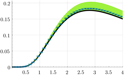
(a) Density, few expansion terms

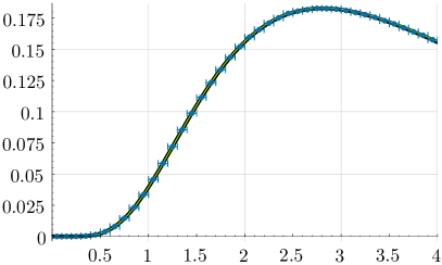
(b) Density, many expansion terms

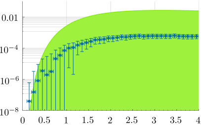
(c) Absolute errors, few expansion terms

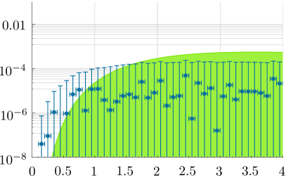
(d) Absolute errors, many expansion terms

Figure 1: The distribution for $20$ $\chi^{2}$ random variables. Figure (a) shows the density compared to an empirical histogram distribution. Figure (c) shows the absolute predicted error vs. the true error, compared to the histogram distribution. (b) and (d) is are the same, with more expansion terms. Note that the uncertainty in the histogram distribution is—due to computational restrictions—huge.

One way of checking our results quantitatively is comparing them to Monte Carlo simulations, namely building a histogram distribution from a table of drawn values. This will only work in the regime with a lot of mass in the distributions, the tails will not receive enough data points to be quantitatively correct.

In figure 1, you can see the density for $n=20$, where the weights were taken from equation 9. Depending on the threshold that is taken for the error bound, equation 5, the expansion comes arbitrarily close to the empirical distribution. Note that the error bound shrinks accordingly and—as expected—we only have an error in the positive $y$ direction. Also observe that our error bound still vastly overestimates the true error.

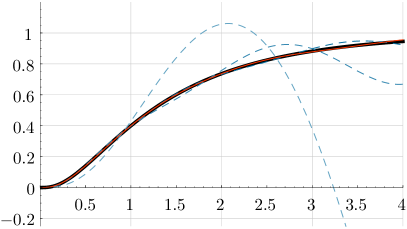
(a) Laguerre expansion

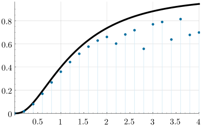
(b) Numerical integration

Figure 2: The cumulative distribution for $6$ $\chi^{2}$ random variables. Figure (a) shows an expansion in Laguerre polynomials as proposed by [11], with $1$, $6$, $11$ (blue, dashed) and $16$ (orange, overlays thick black line) expansion terms. Figure (b) shows a numerical integration proposed by [3]. The black line is my method, which is exact at the shown resolution.

In figure 2, my method is compared to two more recently published techniques, where the six weights are again taken from equation 9. The series expansion (a) can be made quite accurate (although the error bound—not shown—is very bad and suggests we expand to much higher order), at the cost of exponentially growing computation time. For more than $10$ terms, it seems impossible to expand to high enough order in any sensible time.

On the other hand, the numerical integration—performed with Mathematica’s adaptive quasi Monte Carlo method with about $10^{5}$ integrand evaluations—suffers from severe convergence problems.

Just as a comparison: The Laguerre expansion takes about $10$ seconds for $16$ terms, the numerical integration about $250$ seconds (for all the values shown—for a single value it is about $10$ seconds), whereas my method needs about $0.2$ seconds. While not representative, this should give a rough idea of what to expect; they were all run on one i7-2670QM core. While it is true that implementing the Laguerre expansion or the numerical integration in C could be orders of magnitudes faster, mind that our method is executed by Mathematica, too.

5 Counting String Vacua

5.1 Background and Motivation

String theory admits some $10^{500}$ vacuum solutions—for an interesting digression, see [16]. They emerge from the parameter space describing the internal compact manifold, which string theory requires in addition to our $3+1$ dimensional spacetime. This parameter space is called the moduli space of supersymmetric vacua. At low energies, these moduli appear as massles scalar fields with their own equations of motion and potential.

The question of how many of those configurations correspond to physically stable solutions is an active field of research. One vacuum configuration—a deSitter spacetime—is particularly physically motivated, since it agrees with the recent discovery of an accelerated expanding universe.

A more recently published work by [17] analytically calculates the probability of metastable vacua in exactly supersymmetric scenarios.

In a general supersymmetric AdS vacuum, all the masses are bigger than the Breitenlohner-Freedman bound, which is $m_{min}^{s}=-\frac{9}{4}|W|^{2}<0$ in four dimensions (see $2.7$ in [17]). Thus the probability that all masses are positive, has been calculated to go as

$$P_{N}=\exp(-c_{2}N^{2})\quad\text{where}\quad c_{2}=2\frac{|W|^{2}}{m_{\mathrm{susy}}^{2}}\quad,$$

where $W$ denotes the superpotential. By tuning this parameter $W/m_{\mathrm{susy}}$ accordingly, one can make the probability of tachyonic directions either arbitrarily small or large—the interesting question is what a typical value of this parameter is. Some answers to this question can also be found in [17].

In [4], $W$ and $F_{I}={\cal D}_{I}W$ are very small, approaching a supersymmetric Minkowski vacuum, where there is no supression—we have $W\equiv 0$ and all masses are positive. But since the authors want to keep a deSitter vacuum—i.e. only approximately approach a Minkowski vacuum—the sGoldstino in general has a negative mass. What was calculated in [4] was the probability that this direction is not tachyonic. One important point to notice is that it is not at all obvious that deSitter vacua arising from spontaneous symmetry breaking are much more common than deSitter vacua from uplifting of a supersymmetric AdS vacuum. This question has to be addressed by calculation and is not something we know a priori.

Following the work of [4], in the study of $\mathcal{N}=1$ supergravities, it was shown that the fraction of metastable deSitter vacua shrinks exponentially with the number of scalar fields $N\gg 1$. By constructing a random matrix model for the Hessian matrix $\mathbf{H}$ of the scalar potential and calculating its eigenvalue spectrum, local minima can be found.

The suggested functional dependence for $N$ fields for the probability of the smallest eigenvalue fluctuating to a positive value—which renders $\mathbf{H}$ positive definite—was

$$P_{N}\propto\exp\left(-cN^{p}\right)\quad\mathrm{where}\quad c,t>0\quad.$$ (6)

The Hessian matrix can be block-diagonalized to $\mathbf{H}=\mathrm{diag}(m_{-},m_{+})$, where $m_{\pm}$ denotes a mass matrix. An important result is the explicit expression for the smallest eigenvalue of the mass matrix,

$$m_{\pm}^{2}=F^{2}\mathcal{T}_{\pm}-F^{2}\mathcal{S}\quad.$$

$\mathcal{T}_{\pm}$ and $\mathcal{S}$ are given by

$$\mathcal{T}_{\pm} =\frac{2}{3}\omega^{2}+K_{11}^{e}K_{\bar{1}\bar{1}e}-K_{1\bar{1}1\bar{1}}\pm\underbrace{\left|U_{111}F^{-1}\mathrm{e}^{-\theta_{F}}-\frac{2}{3}\omega^{2}\mathrm{e}^{2\mathrm{i}(\theta_{F}-\theta_{W})}\right|}_{=:|t_{\mathrm{hol}}|}\quad,$$ (7)

$$\mathcal{S} =\sum_{b^{\prime}=2}^{N}\frac{|U_{11b^{\prime}}|^{2}}{\lambda_{b^{\prime}}^{2}}$$ (8)

where

$$\omega =\frac{\sqrt{3}}{F}|W|\quad\mathrm{and}\quad F\propto\frac{1}{\sqrt{N}}\quad.$$

Here, $K$ denotes the Kähler potential and $W$ the superpotential, which are taken to be random functions. $U$ and $F$ are derivatives of $W$. It was claimed in [4] that the statistical properties of $\mathcal{T}_{\pm}$ can be neglected for large $N$ and replaced by its expectation value, i.e. $\mathcal{T}_{-}\approx 1$. While qualitatively correct for the limiting distribution, this approximation neglects a number of important aspects, so let us revisit this argument briefly.

The first term in $\mathcal{T}_{-}$, $\omega^{2}$, does not depend on $N$ and we can thus ignore it, since we rescale our results anyways—for $\omega\in[0,1]$, the introduced error is negligible. The term $-|t_{\mathrm{hol}}|$ is indeed negative semi-definite, and for a conservative estimate we can set $|t_{\mathrm{hol}}|$ to $0$, as expained in [4].

For $|K^{(3)}|^{2}$, which is distributed as $\frac{1}{N}\chi^{2}_{N}$ with $\langle|K^{(3)}|^{2}\rangle=1$, it was claimed that the fluctuation probability is negligible for large $N$, stating the central limit theorem. While certainly correct for very large $N$, distributions with nonzero skewness tend to converge slowly to a normal distribution. Furthermore, the width of this process scales as $N^{-1/2}$. The same argument holds true for the third term in equation 7, $K_{1\bar{1}1\bar{1}}^{(4)}\sim\mathcal{N}(0,N^{-1/2})$, so even for large $N=\mathcal{O}(10^{3})$, fluctuation of these two terms cannot be dismissed.

B contains an overview over the different terms comprising $m^{2}_{-}$ where the just-mentioned points can be seen explicitly. Comparing the convolutions from the middle and right column, the reader can observe that the fluctuation probability of the $\mathcal{T}$-term indeed plays an important role, and still affects the overall magnitude quite significantly, even for larger $N$.

For the sake of demonstrating the usefulness of our method to the present problem, however, we will revert temporarily to ignoring the $\mathcal{T}$-terms and try to calculate the leading contribution to the fluctuation probability of $m^{2}_{-}$, i.e. $\mathds{P}(\mathcal{S}\leq 1)$. We will reintroduce the $\mathcal{T}$ contributions in the next section.

The $U_{11b^{\prime}}$ are $N-1$ independent and identically normally distributed random variables $\sim\mathcal{N}(0,1)$, while the denominators $\lambda_{b^{\prime}}^{2}$ are determined by the Marčenko-Pastur law

$$f_{\mathrm{MP}}(\lambda)=\frac{1}{2\pi\lambda N\sigma^{2}}\sqrt{\lambda\left(4N\sigma^{2}-\lambda\right)}\quad\mathrm{where}\quad\sigma=\frac{1}{\sqrt{N}}\quad.$$ (9)

It can be justified to take the weights $\lambda_{b^{\prime}}^{-2}$ such that

$$\lambda_{b^{\prime}}^{2}=\left<\lambda_{b^{\prime}}^{2}\right>\quad\mathrm{:}\quad\int_{0}^{\left<\lambda_{b^{\prime}}^{2}\right>}f_{\mathrm{MP}}(\lambda)\mathrm{d}\lambda=\frac{b^{\prime}}{N}\quad.$$ (10)

This corresponds to numerically inverting the function $f_{\mathrm{MP}}$ on the range $(0,4)$, which is well defined (unfortunately, this cannot be done analytically). $f_{\mathrm{MP}}$ and the weights for specific $N$ can be seen in figure 3.

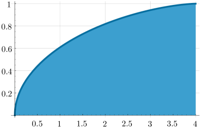
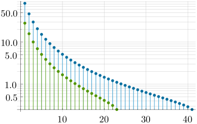
Figure 3: (a) The Marčenko-Pastur law. (b) Weights for $N=24$ and $N=42$, as determined by equation 10.

It is important to point out that the prefactors pose another hard condition on the problem. Rather elegant methods such as the $\chi^{*}$ approach in [18] cannot be used to extract further useful information about this specific case of a linear combination of $\chi^{2}$ random variables, since a closed expression for the prefactors is not known.

In order to calculate the fluctuation probability $\mathds{P}(\mathcal{S}\leq 1)$, we need to know the distribution of $\mathcal{S}$, which is a linear combination of iid $\chi^{2}_{1}$ random variables. In [4], a three moment fit ([5]) is used to approximate the distribution with a single $\chi^{2}_{p}$ variable—the quality of which we will discuss later. The computed values were

$$p \approx 0.24\quad\mathrm{and}\quad c\approx 23\quad.$$

In contrast, by simulating the full mass matrix $$m^{2}_{-} N$$ numerically and then fitting the -dependence to equation 6, the values

$$p =1.28\pm 0.10\quad\mathrm{and}\quad c=0.29\pm 0.06$$

were obtained. The difference is significant.

5.2 Simulation

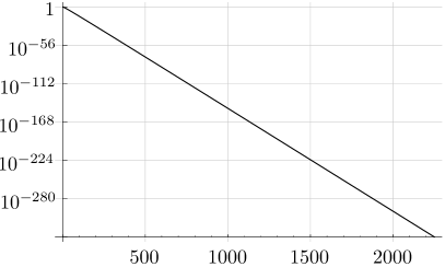
(a) $P_{N}$

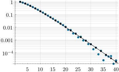
(b) Comparison with [4]

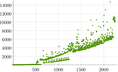
(c) Computation time (in s)

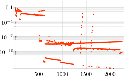
(d) Relative errors

Figure 4: Figure (a) shows the $N$ dependence of $P_{N}$. Figure (b) shows that the result is coherent with the simulation of the $\mathcal{S}$-terms of the mass matrix, as done by [4]. Figure (c) shows the computation time needed to calculate the values and (d) the relative errors, as determined by the algorithm.

Let us return to the issue of finding the $N$ dependence of the fluctuation probability of the mass matrix in our $4d$ random supergravity. For now accepting the approximation $\mathcal{T}_{-}\approx 1$, we want to calculate

$$P_{N}:=\mathds{P}\left(F^{2}\sum_{b^{\prime}=2}^{N}\frac{|U_{11b^{\prime}}|^{2}}{\left<\lambda_{b^{\prime}}^{2}\right>}\leq 1\right)=:\mathds{P}\left(\sum_{i=2}^{N}a_{i}X_{i}\leq 1\right)=:\mathds{P}(Y_{N}\leq 1)\quad,$$ (11)

where $X_{i}\sim\chi^{2}(1)$ and $a_{i}:=(N\left<\lambda_{b^{\prime}}^{2}\right>)^{-1}$.

Using the method discussed in section 2, we calculate the pdf $f_{Y_{N}}$ for $N$ from $2$ to $2250$ and integrate it over $(0,1)$, which gives $P_{N}$. All the while the simulation keeps track of the relative error and ensures that it stays below $0.05$. The results can be seen in figure 4.

The first $400$ values were calculated on a single i7-2670QM, while the rest were computed on a small cluster with slower individual CPUs (i7-860) and varying load balance, which is where the big amount of noise for the computation time and the relative errors originates.

Let us now return to the question of the distribution of the full mass matrix $m^{2}_{-}$. Our first observation is that we can analytically convolve the distributions of $|K^{(3)}|^{2}$ and $K_{1\bar{1}1\bar{1}}^{(4)}$. This yields the rather ugly-looking expression

$$f_{\mathcal{T}}(x)=2^{-\frac{n}{4}-2}N\ \mathrm{e}^{-\frac{1}{8}N^{2}x^{2}} \left(\frac{\sqrt{2}\,_{1}\mathrm{F}_{1}\left(\frac{N}{4};\frac{1}{2};\frac{1}{8}(Nx-2)^{2}\right)}{\Gamma\left(\frac{N+2}{4}\right)}\right.$$

$$+\left.\frac{(Nx-2)\,_{1}\mathrm{F}_{1}\left(\frac{N+2}{4};\frac{3}{2};\frac{1}{8}(Nx-2)^{2}\right)}{\Gamma\left(\frac{N}{4}\right)}\right)\quad,$$

which however simplifies gravely for specific values of n. This pdf, alongside the analytical expressions found for the $\mathcal{S}$-term $f_{Y_{N}}$, allows us to numerically convolve the two terms and calculate the distribution—and thus the fluctuation probability—of the full mass matrix, for large numbers of $N$ and to a very high precision.

The numerical convolution is done in a straightforward manner using Mathematica. While estimating the error of such a numerical convolution is generally hard, using small enough sample sizes should give us in principle negligible contribution to our error—we mention it for the sake of completeness though. The results can be seen in figure 6.

5.3 Data Analysis

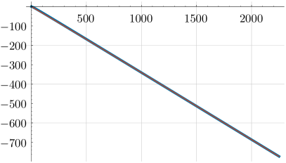
(a) Fit to $-cN^{p}$

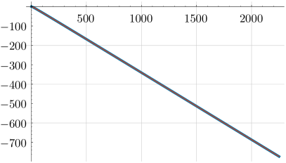
(b) Fit to $\log(a+N)-c-dN$

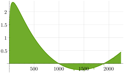
(c) Residuals for (a)

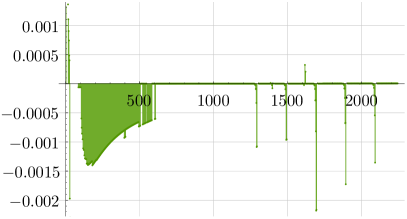
(d) Residuals for (b)

Figure 5: Figure (a) and (b) show plots of fits (orange) to our data (blue) for both proposed models. Figure (c) and (d) show the corresponding residuals.

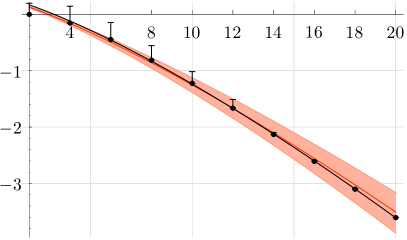
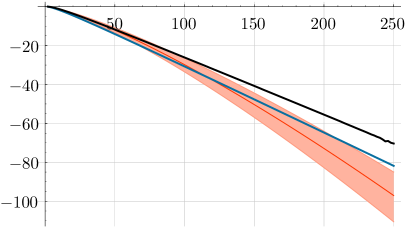
Figure 6: (a) Comparison with [4, Fig. 7]. The shaded area indicates the parameter range for the best fit curve given in [4]. The black line is a similar best fit curve (to the values shown) with $p\approx 1.31$, so well within the error range. (b) Comparison of $\mathds{P}(\mathcal{S}\leq 1)$ (blue), the full $m^{2}_{-}$ (black) and the suggested best fit from [4]. The error bars for our method are negligibly small.

We now turn to the data analysis of our simulation of $\mathcal{S}$ resp. the full mass matrix $m^{2}_{-}$. Our simulation of $\mathcal{S}$ agrees very well with the numerical simulations of the $\mathcal{S}$-part of the mass matrix from [4], as can be seen in the low $N$ regime figure 4(b). For larger $N$, figure 4(a), the overall shape then follows more and more that of a simple exponential, i.e. $\propto\mathrm{e}^{-cN}$ for some $c$.

Indeed, by fitting the suggested functional dependence $\mathrm{e}^{-cN^{p}}$, the residuals show a strong characteristic shape, see figure 5. While the overall shape matches pretty well, another function,

$$\mathrm{e}^{\log(a+N)-c-dN}\equiv(a+N)\mathrm{e}^{-c-dN}\quad,$$ (12)

matches the shape a lot better, as can be seen by looking at the corresponding residuals. While figure 5(d) still shows a correlation for the residuals, they are now of the same order as the proposed error, figure 4(d). This means that this model is correct, within the given precision.

The fit parameters and standard deviations for both models can be found in table 1.

	Estimate	Standard Error
$c$	0.31395	0.00011
$p$	1.01171	0.00005

(a) Parameters for $-cN^{p}$

	Estimate	Standard Error
a	1.88	0.06
c	0.75652	0.00011
d	0.34657360	$4\cdot 10^{-8}$

(b) Parameters for $\log(a+N)-c-dN$

Table 1: Fit parameters for both proposed models for $\mathds{P}(\mathcal{S}\leq 1)$.

	Estimate	Standard Error
$c$	0.186	0.00012
$p$	1.0759	0.00013

(a) Parameters for $-cN^{p}$

	Estimate	Standard Error
a	0.4	0.6
c	0.615	0.013
d	0.30096	$6\cdot 10^{-5}$

(b) Parameters for $\log(a+N)-c-dN$

Table 2: Fit parameters for both proposed models for the full mass matrix $m^{2}_{-}$.

There is an enormous difference in the amount of data available between the aforementioned methods and our newer one. In our paper—and this agrees with [4] and [19]—the first $\mathrm{O}(20)$ data points show a sharp downward bent in a logarithmic plot, suggesting that the probability should go like $P\propto e^{-c_{1}N^{p}}$ with $p\gtrsim 1.25$ (and indeed a fit to those first $20$ points yields just such a behaviour).

However—and this again can already be seen as trend in [4] and [19]—the data points flatten more and more, becoming more and more linear. Unfortunately, the above-mentioned authors did not have sufficiently accurate data for this regime to explore this behaviour. Due to the sheer number of data points in our model ($\mathrm{O}(2000)$), the behaviour at low $N$ does not receive much weight. Since we are interested in high $N$, though, this should not pose a problem.

For the full mass matrix, for which we added in the $N$-dependence of the $\mathcal{T}$-term, we once again basically confirm what has been done in [4], at least in the lower $N$ regime that was accessible for them. In figure 6-a, we see that we can reproduce the previous value of $p\approx 1.3$. Analogously to the case of $\mathcal{S}$ alone, though, for higher values of $N$, the fluctuation probability for $m^{2}_{-}$ to become positive flattens significantly. Repeating the same numerical fit procedure as for the $\mathcal{S}$-term alone, we obtain the fit parameters in table 2.

This is the major result of the application of our method to the open problem of a full stability analysis of deSitter vacua in string theory. In brief, it suggests that the probability of finding a metastable deSitter vacuum follows the asymptotic form P_N∼Ne^-0.30096 ±6⋅10^-5N .

6 Conclusions and Future Work

The first main result is the analytic expression for the density of a sum of two $\Gamma$ random variables (lemma 1). With this expression as a building block, we have derived an efficient algorithm (lemma 2) for the calculation of a linear combination of an even number of $\chi^{2}_{r}$ random variables.

Unfortunately, at this point, the authors were not able to calculate the numerical convolution of the full mass matrix $m_{-}^{2}$ to $N=\mathrm{O}(2000)$ due to computational restrictions. Qualitatively, though, it is clear that the value for $p$ will most likely converge to something in the range $1\lesssim p\lesssim 1.08$.

With these methods, a reliable estimate for the probability of a metastable deSitter vaccum in a $\mathcal{N}=1$ $4d$ supergravity has been shown to be of the asymptotic form $N\mathrm{e}^{-0.3N}$, where $N$ denotes the number of scalar fields in the theory. As discussed, this last result gives a much weaker bound than the one suggested by [4] or [19].

This result is significant. One important implication for the existence of flux vacua is the following. If we assume that there are $M\in\mathrm{O}(10^{500})$ local extrema, of which $M_{+}\ll M$ are metastable deSitter vacua, we can conclude that

$$\log(a+N)-c-dN\sim\log N-dN\sim\log\left(\frac{M_{+}}{M}\right)\quad.$$

Consequently, this description of a $4d$ random supergravity is plausible—i.e. $M_{+}>1$, which means that there is at least one metastable vacuum—if $-500\log 10\lesssim\log N-dN$ or $N\lesssim 3800$.

Appendix  A More Exact Formulae for $\chi^{2}$ Random Variables

There are a few more analytic expressions for the pdf $f$ of a sum of $\chi^{2}$ random variables.

Remark 5.

Let $X,Y,Z\sim\chi^{2}_{1}$ iid random variables and $a,b\in\mathds{R}_{>0}$. Then

$$f_{aX+aY+bZ}(x) =\theta(x)\sqrt{\frac{1}{\pi a^{2}b}}\sqrt{\frac{b-a}{ab}}\ \mathrm{e}^{-\frac{x}{2b}}\mathrm{F}\!\left(\!\!\sqrt{\frac{b-a}{2ab}x}\right)$$

$$\equiv\theta(x)\sqrt{\frac{1}{4a^{2}b}}\sqrt{\frac{b-a}{ab}}\ \mathrm{e}^{-\frac{x}{2a}}\mathrm{erfi}\!\left(\!\!\sqrt{\frac{b-a}{2ab}x}\right)\quad,$$

where $\mathrm{F}$ is the Dawson integral and $\mathrm{erfi}$ the imaginary error function.

Remark 6.

Let $X,Y,Z,W\sim\chi^{2}_{1}$ iid random variables and $a,b\in\mathds{R}_{>0}$. Then

$$f_{aX+aY+aZ+bW}(x)=\theta(x)\frac{1}{4}\frac{1}{\sqrt{a^{3}b}}\mathrm{e}^{-\frac{a+b}{4ab}x}\left(\mathrm{I}_{0}\left(\frac{a-b}{4ab}x\right)+\mathrm{I}_{1}\left(\frac{a-b}{4ab}x\right)\right)\quad.$$

Appendix  B The Fluctuation Probability of the Full Mass Matrix $m^{2}_{-}$

For the full mass matrix $m_{-}^{2}$, we numerically convolved the $\mathcal{S}$ and $\mathcal{T}$-terms and then numerically integrated the probability of getting a positive contribution.

Shown in figure 7 are the different probability density functions for the distributions comprising $m^{2}_{-}$. It is evident to see that the approximation $\mathcal{T}\approx 1$ is quite crude—the fluctuation probability of the $\mathcal{T}$-term plays a certain role, even for larger values of $N$.

2
4
6
8

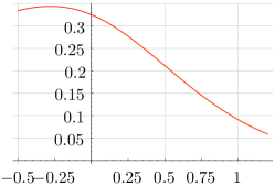
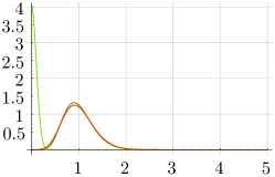
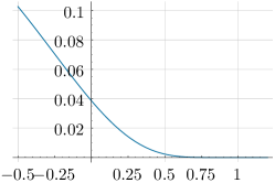
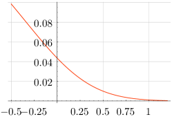
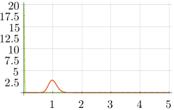
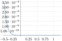
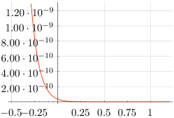
Figure 7: Fluctuation probability for select $N$. Left column: $K_{1\bar{1}1\bar{1}}$ (light green), $K^{(3)}$ (dark green) and their convolution (red). Middle column: right tail of distribution for $\mathcal{S}+1$. Right column: right tail of distribution of full mass matrix $m^{2}_{-}$.

$$\vdots$$

20

$$\vdots$$

100

Appendix  C Literature

References

- \providebibliographyfontname\providebibliographyfontlastname\providebibliographyfonttitle\providebibliographyfontjtitle\btxtitlefont\providebibliographyfontetal\providebibliographyfontjournal\providebibliographyfontvolume\providebibliographyfontISBN\providebibliographyfontISSN\providebibliographyfonturl}\providebibliographyfontnumeral\btxselectlanguage\btxfallbacklanguage
- [1] \btxselectlanguage\btxfallbacklanguage
- [2] \btxnamefont\btxlastnamefontMathai, A.\btxauthorcolon \btxjtitlefont\btxifchangecaseStorage capacity of a dam with gamma type inputsStorage capacity of a dam with gamma type inputs. \btxjournalfontAnnals of the Institute of Statistical Mathematics, 34:591–597, 1982.
- [3] \btxnamefont\btxlastnamefontAkkouchi, Mohamed\btxauthorcolon \btxjtitlefont\btxifchangecaseOn the convolution of gamma distributionsOn the Convolution of Gamma Distributions. \btxjournalfontSoochow J. Math., 31(2):205–211, \btxprintmonthyear.April2005long.
- [4] \btxnamefont\btxlastnamefontMarsh, David, \btxnamefontLiam \btxlastnamefontMcAllister\btxandcomma \btxandlong \btxnamefontTimm \btxlastnamefontWrase\btxauthorcolon \btxjtitlefont\btxifchangecaseThe Wasteland of Random SupergravitiesThe Wasteland of Random Supergravities. \btxjournalfontJ. High Energy Phys., 1203:102, 2012. \btxselectlanguageenglish
- [5] \btxnamefont\btxlastnamefontSolomon, Herbert \btxandlong \btxnamefontMichael\btxfnamespacelongA. \btxlastnamefontStephens\btxauthorcolon \btxjtitlefont\btxifchangecaseDistribution of a sum of weighted chi-square variablesDistribution of a Sum of Weighted Chi-Square Variables. \btxjournalfontJ. Amer. Statist. Assoc., 72(360):pp. 881–885, 1977. \btxselectlanguage\btxfallbacklanguage
- [6] \btxnamefont\btxlastnamefontBruce G. Lindsay, Ramani\btxfnamespacelongS.\btxfnamespacelongPilla \btxandlong \btxnamefontPrasanta \btxlastnamefontBasak\btxauthorcolon \btxjtitlefont\btxifchangecaseMoment-based approximations of distributions using mixtures: Theory and applicationsMoment-based approximations of distributions using mixtures: Theory and applications. \btxjournalfontAnn. Inst. Statist. Math., 52(2):pp. 215–230, 2000.
- [7] \btxnamefont\btxlastnamefontWood, Andrew\btxfnamespacelongT.\btxfnamespacelongA., \btxnamefontJames\btxfnamespacelongG. \btxlastnamefontBooth\btxandcomma \btxandlong \btxnamefontRonald\btxfnamespacelongW. \btxlastnamefontButler\btxauthorcolon \btxjtitlefont\btxifchangecaseSaddlepoint approximations to the cdf of some statistics with nonnormal limit distributionsSaddlepoint Approximations to the CDF of Some Statistics with Nonnormal Limit Distributions. \btxjournalfontJournal of the American Statistical Association, 88(422):680–686, 1993.
- [8] \btxnamefont\btxlastnamefontMoschopoulos, P.\btxauthorcolon \btxjtitlefont\btxifchangecaseThe distribution of the sum of independent gamma random variablesThe distribution of the sum of independent gamma random variables. \btxjournalfontAnn. Inst. Statist. Math., 37:541–544, 1985.
- [9] \btxnamefont\btxlastnamefontMoschopoulos, P.\btxauthorcolon \btxjtitlefont\btxifchangecaseThe distribution function of a linear combination of chi-squaresThe distribution function of a linear combination of chi-squares. \btxjournalfontComputers and Mathematics with Applications, 10(4-5):383 – 386, 1984.
- [10] \btxnamefont\btxlastnamefontAkkouchi, Mohamed\btxauthorcolon \btxjtitlefont\btxifchangecaseOn the convolution of exponential distributionsOn the Convolution of Exponential Distributions. \btxjournalfontJ. Chungcheong Math. Soc., 21(4):501–510, \btxprintmonthyear.December2008long.
- [11] \btxnamefont\btxlastnamefontCastaño-Martínez, Antonia \btxandlong \btxnamefontFernando \btxlastnamefontLópez-Blázquez\btxauthorcolon \btxjtitlefont\btxifchangecaseDistribution of a sum of weighted noncentral chi-square variablesDistribution of a sum of weighted noncentral chi-square variables. \btxjournalfontTEST, 14:397–415, 2005. \btxselectlanguageenglish
- [12] \btxnamefont\btxlastnamefontFleiss, Joseph\btxfnamespacelongL.\btxauthorcolon \btxjtitlefont\btxifchangecaseOn the distribution of a linear combination of independent chi squaresOn the Distribution of a Linear Combination of Independent Chi Squares. \btxjournalfontJ. Amer. Statist. Assoc., 66(333):pp. 142–144, 1971. \btxselectlanguage\btxfallbacklanguage
- [13] \btxnamefont\btxlastnamefontDavies, Robert\btxfnamespacelongB.\btxauthorcolon \btxjtitlefont\btxifchangecaseThe distribution of a linear combination of chi-squared random variablesThe distribution of a linear combination of chi-squared random variables. \btxjournalfontJ. Appl. Stat., 29:323–333, 1980.
- [14] \btxnamefont\btxlastnamefontStein, Elias\btxfnamespacelongM. \btxandlong \btxnamefontGuido \btxlastnamefontWeiss\btxauthorcolon \btxtitlefontIntroduction to Fourier Analysis on Euclidean Spaces. \btxpublisherfontPrinceton University Press, 1971.
- [15] \btxnamefont\btxlastnamefontWolfram Web Resources\btxauthorcolon \btxtitlefont\btxifchangecaseKummer confluent hypergeometric function, specialized valuesKummer confluent hypergeometric function, specialized values, 2012. \btxurlfonthttp://functions.wolfram.com/07.20.03.0024.01.
- [16] \btxnamefont\btxlastnamefontSusskind, Leonard\btxauthorcolon \btxjtitlefont\btxifchangecaseThe Anthropic landscape of string theoryThe Anthropic landscape of string theory. 2003.
- [17] \btxnamefont\btxlastnamefontBachlechner, Thomas\btxfnamespacelongC., \btxnamefontDavid \btxlastnamefontMarsh, \btxnamefontLiam \btxlastnamefontMcAllister\btxandcomma \btxandlong \btxnamefontTimm \btxlastnamefontWrase\btxauthorcolon \btxjtitlefont\btxifchangecaseSupersymmetric Vacua in Random SupergravitySupersymmetric Vacua in Random Supergravity. \btxjournalfontJHEP, 1301:136, 2013.
- [18] \btxnamefont\btxlastnamefontLindsay, Bruce\btxfnamespacelongG., \btxnamefontMarianthi \btxlastnamefontMarkatou, \btxnamefontSurajit \btxlastnamefontRay, \btxnamefontKe \btxlastnamefontYang\btxandcomma \btxandlong \btxnamefontShu\btxfnamespacelongChuan \btxlastnamefontChen\btxauthorcolon \btxjtitlefont\btxifchangecaseQuadratic distances on probabilities: A unified foundation.Quadratic distances on probabilities: A unified foundation. \btxjournalfontAnn. Stat., 36(2):983–1006, 2008.
- [19] \btxnamefont\btxlastnamefontChen, Xingang, \btxnamefontGary \btxlastnamefontShiu, \btxnamefontYoske \btxlastnamefontSumitomo\btxandcomma \btxandlong \btxnamefontS.H.\btxfnamespacelongHenry \btxlastnamefontTye\btxauthorcolon \btxjtitlefont\btxifchangecaseA Global View on The Search for de-Sitter Vacua in (type IIA) String TheoryA Global View on The Search for de-Sitter Vacua in (type IIA) String Theory. \btxjournalfontJ. High Energy Phys., 1204:026, 2012.