Discussion of “Multiple Testing for Exploratory Research” by J. J. Goeman and A. Solari

10.1214/11-STS356

I want to congratulate the authors on this thought-provoking and important paper on multiple testing in exploratory settings.

Standard Multiple Testing procedures can appear very mechanistic. Hypotheses are ordered by increasing $p$-value. Given a Type I error criterion, the Multiple Testing procedure selects a cut-off in this list. Simply working down the list of hypotheses in order of their $p$-values is perhaps suboptimal for exploratory analysis as a lot of information is lost in this way and important discoveries might be missed. Some previous work has addressed this issue bychanging the ranking of the hypotheses. To highlight only three examples: Tibshirani and Wasserman (2006) devised a method to borrow strength across highly correlated test statistics in microarray experiments. Storey (2007) proposed an “optimal discovery” procedure that again leads to a different ranking of variables than the ranking implied by the marginal $p$-values. One of the authors also proposed a very powerful way of incorporating known network structure into the testing procedure [Goeman and Mansmann, 2008].

The proposed approach to exploratory multiple testing is more radical, though, than changing the cut-off or changing the ranking of hypotheses. Instead of the perhaps rather dull task of selecting a cut-off in a list of ordered hypotheses, the researcher can reject for follow-up analysis any set of hypotheses he or she regards as interesting, using all the information at hand. The method then returns a lower bound on the number of false null hypotheses (true discoveries) in this set. Since the bound is valid simultaneously across all sets, an exploratory approach does not invalidate the error bound.

I think this method will be very important and useful in many fields as it allows a flexible exploration of possibly interesting sets of hypotheses, while at the same time protecting the practitioner against too many false rejections (or at least managing expectations about the number of true discoveries one can hope to make).

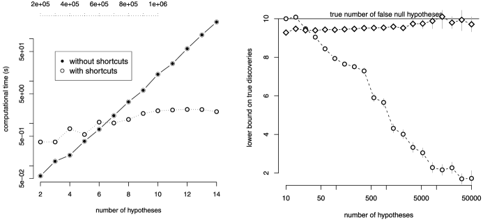
Figure 1: Left: computational time (on log-scale) for the standard approach in regression (solid line), with the number of hypotheses ranging from 2 to 12, and computational time for the shortcut for independent tests (dotted line), with the number of hypotheses between $2\cdot 10^{5}$ and $1.2\cdot 10^{6}$. Only the latter is feasible for large-scale testing. Right: the average lower bound on the total number of true discoveries with the proposed approach (circles) and an alternative given in the text (diamonds). Due to the simultaneous nature of the proposed bounds, the overall power to reject is good for a few dozen hypotheses but is deteriorating as the number of hypotheses grows into the hundreds.

There is a price to be paid for the simultaneous nature of the bound, though. I have some doubts (hopefully unfounded) about the applicability tolarge-scale testing situations as they arise, for example, in genomics or astronomy for two reasons: computational complexity and statistical power.

It is obvious and also acknowledged by the authors that the proposed procedure without shortcuts will be impractical for even just a few dozen hypotheses. The computational complexity is simply too high. An example is shown in Figure 1 for a genomics regression example with less than one hundred observations. The proposed method takes already more than half a minute for 12 predictor variables on a standard computer with a 3 GHz CPU and the supplied cherry R-package and the complexity seems to be (super-)exponential in the number of hypotheses, as one would expect. The proposed shortcuts are not applicable in all settings. If they are applicable, they seem to be very effective in reducing the computational complexity, making large-scale testing feasible. Figure 1 shows that even testing situations with $>10^{6}$ tests are handled in about a second or less.

Maybe more worrying, the statistical power of the method deteriorates with an increasing number of hypotheses. This is due to the simultaneous nature of the bound on the number of correctly rejected hypotheses among all possible sets of hypotheses. I compared the power for a simple setting, in which there are $m$ independent $p$-values $p_{i}$ with $i=1,\ldots,m$ with distribution $p_{i}\sim U([0,c_{i}])$ and $c_{i}=1$ if $i>10$ and $c_{i}=0.1/m$ if $i\leq 10$ (there are hence 10 false null hypotheses). If rejecting all hypotheses, the lower bound for the number of correctly rejected hypotheses is shown as a function of $m$ in Figure 1, along with the bound for the same quantity proposed by Meinshausen and Rice (2006). The proposed approach works very well up to a few dozen hypotheses. If the number of hypotheses is in the hundreds, the number of sets the bound needs to be valid over is getting so large that the power of the method starts to deteriorate quickly.

I acknowledge that the comparison is not quite fair since the method in Meinshausen and Rice (2006) does much less: it only gives a lower bound on the total number of false null hypotheses or a lower bound for the number of true discoveries in a list that is ordered by increasing $p$-values of the hypotheses. [If we were to ask only if there are any false null hypotheses at all, we could be even more sensitive to deviations from the global null hypothesis with Higher Criticism (Donoho and Jin, 2004).] And for fewer than 50 hypotheses, the proposed bound is remarkably good.

The power and computational cost objectives thus both indicate that the method is working very well for up to a few dozen hypotheses but will probably need refinements for large-scale testing.

A thought regarding the presentation of results. As proposed, the method acts somewhat like a black-box: if given a set of hypotheses, it returns a lower bound on the number of true discoveries within this set. While this might be the right approach in many exploratory settings, I also think that many practitioners could use some guidance as to which sets of hypotheses could be interesting (without prescribing exactly which ones to reject, so as to not fall back into the standard ranking scheme). A step in this direction is the helpful concept of defining hypotheses, which summarizes the results of the procedure in compact form.

Each defining hypothesis is a set of hypotheses out of which at least one hypothesis must be a false null hypothesis. In other words: the defining hypotheses have a logical AND–OR connection (with AND between the sets of hypotheses and OR between hypotheses in a set). A complementary view could be given by a logical OR–AND connection, with OR between sets of hypotheses and AND between hypotheses in a set. The results are still presented as sets of hypotheses. Among all these sets and conditional on event $E$, there is now guaranteed to be at least one set such that all hypotheses in this set are false. This extends the usual Multiple Testing paradigm, where the user is handed back just one set of hypotheses, which is guaranteed to be a set of false null hypotheses.

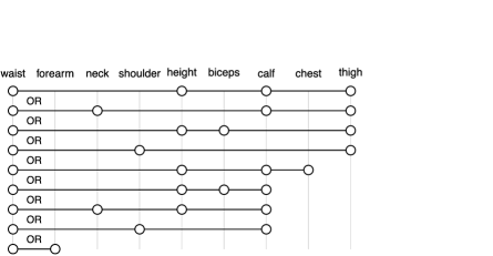
Figure 2: An alternative presentation of the results in the regression example. All dots on each horizontal line form a set of hypotheses. Out of all nine sets, at least one must correspond to a set of false null hypotheses (conditional on event $E$).

In the regression example, there are nine such sets, the first two being {waist, height, calf, thigh} and {waist, neck, calf, thigh}. Figure 2 visualizes them. Among these nine sets, at least one must be a set where all hypotheses are false null hypotheses (always conditional on the event $E$). We can then directly read off that if height is known to be a null hypothesis (either by a follow-up experiment or through prior knowledge), then the results give no reason any longer to suppose that chest was a false null (since chest is only part of the fifth set; and if height is a true null, this set can be excluded and neck will not any longer be in the union of all other candidate sets). Or, if calf can be excluded, then the results do not give reason to still suspect that neck was a false null hypothesis. Such statements and connections are much more difficult to read off the set of defining hypotheses but might be useful in practice, when planning which hypotheses to follow up.

I want to congratulate the authors again on this very impressive and useful paper and I hope to see strong uptake of the method.

References

- (1) {barticle}[mr] \bauthor\bsnmDonoho, \bfnmDavid\binitsD. and \bauthor\bsnmJin, \bfnmJiashun\binitsJ. (\byear2004). \btitleHigher criticism for detecting sparse heterogeneous mixtures. \bjournalAnn. Statist. \bvolume32 \bpages962–994. \biddoi=10.1214/009053604000000265, issn=0090-5364, mr=2065195 \bptokimsref \endbibitem
- (2) {barticle}[pbm] \bauthor\bsnmGoeman, \bfnmJelle J.\binitsJ. J. and \bauthor\bsnmMansmann, \bfnmUlrich\binitsU. (\byear2008). \btitleMultiple testing on the directed acyclic graph of gene ontology. \bjournalBioinformatics \bvolume24 \bpages537–544. \biddoi=10.1093/bioinformatics/btm628, issn=1367-4811, pii=btm628, pmid=18203773 \bptokimsref \endbibitem
- (3) {barticle}[mr] \bauthor\bsnmMeinshausen, \bfnmNicolai\binitsN. and \bauthor\bsnmRice, \bfnmJohn\binitsJ. (\byear2006). \btitleEstimating the proportion of false null hypotheses among a large number of independently tested hypotheses. \bjournalAnn. Statist. \bvolume34 \bpages373–393. \biddoi=10.1214/009053605000000741, issn=0090-5364, mr=2275246 \bptokimsref \endbibitem
- (4) {barticle}[mr] \bauthor\bsnmStorey, \bfnmJohn D.\binitsJ. D. (\byear2007). \btitleThe optimal discovery procedure: A new approach to simultaneous significance testing. \bjournalJ. R. Stat. Soc. Ser. B Stat. Methodol. \bvolume69 \bpages347–368. \biddoi=10.1111/j.1467-9868.2007.005592.x, issn=1369-7412, mr=2323757 \bptokimsref \endbibitem
- (5) {bmisc}[auto:STB—2011/11/23—09:42:52] \bauthor\bsnmTibshirani, \bfnmR.\binitsR. and \bauthor\bsnmWasserman, \bfnmL.\binitsL. (\byear2006). \bhowpublishedCorrelation-sharing for detection of differential gene expression. Arxiv preprint. Available at arXiv:math/0608061. \bptokimsref \endbibitem