Discussion of “Multiple Testing for Exploratory Research” by J. J. Goeman and A. Solari

10.1214/11-STS356

1 Initial Comments

Closure-based multiple testing procedures for controlling the familywise error rate (FWER) have been around for decades, but they have not been well understood, and hence have been under-appreciated and under-utilized. Goeman and Solari (GS) provide a service by highlighting important practical features of closure. Using elegant notation for closure-based methods, they develop a handy book-keeping tool for presenting additional results of closed testing that are available when non-consonant testing methods are used, and they prove its validity.

In their Figure 1, GS provide the confidence set $\tau(\{2,3\})\in\{0,1\}$, where $\tau(\{2,3\})$ is the number of true nulls in the set $\{H_{2},H_{3}\}$. In doing so, GS highlight a not-so-well known fact about closure: inferences for the additional $(2^{n}-1)-n$ composite hypotheses $H_{I}$ are available “free of charge” whenever one performs closed testing for the original $n$ elementary hypotheses $H_{i}.$ This follows from the fact that “the closure of the closure is the closure;” that is, that no new hypotheses are generated when the set of $2^{n}-1$ intersection hypotheses is treated as the set of elementary hypotheses. Hence, in GS’s Figure 1, the significance of $H_{\{2,3\}}$ can be stated with full FWER control over the set of $2^{3}-1=7$ hypotheses, and the conclusion $\tau(\{2,3\})\leq 1$ follows immediately. Again, GS provide a service in reminding statisticians (or in teaching those who have not heard about it in the first place) of this nice feature of closure.

GS’s paper also implicitly explains the following paradox: while closure is based on composite hypotheses, it is not true that more powerful composite tests lead to more powerful closure-based multiple tests. When considering only the elementary hypotheses, Bonferroni (or MaxT) types of composite tests, which are usually thought to be the least powerful of the class of composite testing methods (e.g., Nakagawa, 2004), tend to give higher power for closure-based multiple tests (Romano, Shaikh and Wolf, 2011). However, when the goal is to establish how many true effects there might be among a collection of hypotheses, GS suggest indeed that more powerful composite tests lead to more powerful multiple tests.

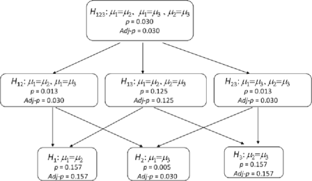
Figure 1: Closed testing with Fisher combination tests in a one-way ANOVA setting, ignoring logical constraints.

The Fisher combination test is a useful choice of composite test, as noted by GS. But it is worth pointing out how bad this test can be compared to the Bonferroni test, when both are used via closure for testing elementary hypotheses. Consider analyzing a version (available from the author) of the classic dataset reported by Golub at al. (1999), testing 7,129 genes for association with either acute myeloid or acute lymphoblastic leukemia, using 7,129 two-sample $t$-tests. The closed Fisher combination method is and has been available in PROC MULTTEST of SAS/STAT with the $O(n^{2})$ shortcut since release 8.1 of SAS in 2000; this software computes closure-based adjusted $p$-values (defined below) to assess significance of elementary hypotheses. Despite the fact that the Fisher combination test is liberal with correlated data, the smallest adjusted $p$-value using the closed Fisher combination test is $1.000$ (rounded), hence none of the 7,129 tests are significant at any reasonable nominal FWER level. On the other hand, 37 of the 7,129 genes have adjusted $p$-values less than the nominal 0.05 FWER level when using closed Bonferroni (or Holm, 1979) tests; the smallest adjusted $p$-value is $1.7\times 10^{-6}$ and is therefore extremely significant, even after multiplicity adjustment.

I have some other comments/critiques about the paper that fall into the following categories: (i) the assumption of free combinations and its consequences, (ii) use of adjusted $p$-values rather than rigid nominal thresholds, (iii) computational shortcuts, and (iv) permutation testing.

2 Additional Comments

2.1 Free Versus Restricted Combinations

Implicit in GS’s discussion of closure is that the elementary hypotheses obey the free combinations condition, which states that there are $2^{n}-1$ distinct hypotheses in the closure. Under restricted combinations there are duplicates, and hence the set of intersections has many fewer elements; by exploiting this fact one can obtain tighter confidence sets. For example, suppose $Y_{i}\sim N(\mu_{i},1)$, with $H_{1}\dvtx\mu_{1}=\mu_{2}$, $H_{2}\dvtx\mu_{1}=\mu_{3}$ and $H_{3}\dvtx\mu_{2}=\mu_{3}$. Then there are only four elements in the closure rather than $2^{3}-1=7$, since $H_{\{1,2\}}=H_{\{1,3\}}=H_{\{2,3\}}=H_{\{1,2,3\}}$. GS’s method is valid but conservative when all seven hypotheses are considered.

For example, suppose the data are $y_{1}=-2$, $y_{2}=0$ and $y_{3}=+2$, yielding $z$-statistics $z_{1}=(-2-0)/\break 2^{1/2}=-1.414,$ $z_{2}=-2.828$ and $z_{3}=-1.4141$, with corresponding two-sided $p$-values $p_{1}=0.157299$,$p_{2}=0.004678$ and $p_{3}=0.157299$. The Fisher combinations statistics are thus $c_{12}=c_{23}=-2\times\break\ln(0.157299\times 0.004678)=14.4291$, $c_{13}=7.3984$ and $c_{123}=18.1283$. The chi-squared distribution cannot be used to find $p$-values for these composite tests since the $Z$’s are not independent, but under the null hypothesis, the vector of $Z$ statistics is multivariate normal with mean vector $\biggl{[}{\matrix{{0}\cr{0}\cr{0}}}\biggr{]}$ and covariance matrix $\biggl{[}{\matrix{1&0.5&-0.5\cr 0.5&1&0.5\cr-0.5&0.5&1}}\biggr{]}.$ Thus, the $p$-values can be obtained by simulating $Z$’s from this distribution, computing the two-sided $p$-values, constructing the Fisher combination statistics $C_{I}$, and counting how often the simulated $C_{I}$ exceeds the observed $c_{I}$. Figure 1 displays the results using these $p$-values for each subset $I$, as well as closure-based adjusted $p$-values.

Suppose that inference is considered for the set $\{H_{1},H_{3}\}$. Here, the confidence set for the number of true nulls is $\{0,1,2\}$, since $H_{13}$ is not rejected. But the possibility that $\tau(\{1,3\})=2$ contradicts the rejection of the global hypothesis $H_{123}$, and thus seems wrong.

Incorporating logical constraints, the graph is as shown in Figure 2. Using logical constraints, the confidence set for $\tau(\{1,3\})$ is $\{0,1\}$ rather than $\{0,1,2\}$.

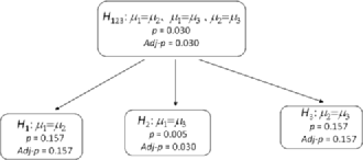
Figure 2: Closed testing with Fisher combination tests in a one-way ANOVA setting, incorporating logical constraints.

One can improve the power of closure-based consonant procedures as well by utilizing logical constraints (Westfall and Tobias, 2007).

2.2 Adjusted $p$-Values

Adjusted $p$-values are simple and natural by-products of closure. Let $p_{I}$ be the local $p$-value for testing $H_{I}$. With closure, $H_{I}$ is rejected only when $H_{J}$ is rejected for all $J\supseteq I$, or equivalently, when$\max_{J\supseteq I}p_{J}\leq\alpha$, where $\alpha$ is the nominal FWER.Hence $\max_{J\supseteq I}p_{J}$ is the adjusted $p$-value for testing $H_{I}$, and these are shown in my Figure 1.

As GS note, exploratory inference should be mild, flexible and post hoc. However, the use of a strict $0.05$ (or other) nominal FWER threshold seems to violate the latter two of these criteria. For the same reasons that ordinary $p$-values are seen as more natural and useful than the $0.05$-level determined “accept/reject” decision, it is also more natural and useful to report an adjusted $p$-value along with any claim about the number of true alternatives within a set of hypotheses.

For example, suppose my Figure 1 was from a case of free combinations, as with GS’s Figure 1. Then for the set $\{H_{1},H_{3}\}$, one cannot claim any alternatives at the usual $0.05$ nominal FWER level, but one can conclude at least one alternative at the nominal $0.13$ level. The report could state “For familywise significance levels as low as $0.125$, there is at least one alternative among $\{H_{1},H_{3}\}$.”

In GS’s discussion of Huang and Hsu’s $n=4$ example where there are no elementary significances, their conclusion is “at least two out of the first three hypotheses are false.” After calculating the adjusted $p$-values for these data, one can say “at least two out of the first three hypotheses are false (adjusted $p=0.038$).” With other data, the conclusion might be that “at least two out of the first three hypotheses are false (adjusted $p=0.001$),” which communicates quite different information, even though the claimed number of alternatives is the same at the nominal FWER${}=0.05$ level.

Yet another benefit of adjusted $p$-values is that they offer a more realistic assessment in the face of violated assumptions. Assumptions are usually wrong, and an adjusted $p$-value of $0.055$ might be more appropriately reported as $0.041$ with a more correct analysis; conversely, $0.045$ might be more appropriately reported as $0.053$. Use of adjusted $p$-values rather than fixed decisions better recognizes this fact, as savvy readers understand that $p$-values are themselves approximations, and can use their own knowledge or simulation studies to assess the accuracy of a “$0.045$” report.

A disadvantage of using adjusted $p$-values rather than “accept/reject” decisions is that there are additional computations. But this disadvantage seems minor to me compared to problems with rigidly fixed nominal FWER levels.

2.3 Computational Shortcuts

The methodology GS espouse can be computationally prohibitive. While closure allows a simple $O(n)$ shortcut in the case of the consonant Bonferroni–Holm procedure, the GS methods will require something approaching $O(2^{n})$ evaluations for most other cases of interest. Shortcuts are available, with less power as GS note. Westfall and Tobias (2007) use a tree-based representation of the $2^{n}-1$ hypotheses, along with a branch-and-bound algorithm for obtaining conservative, but computationally simpler analyses. These methods are available in a wide variety of SAS/STAT procedures as of version 9.2 of SAS.

Oddly, GS do not mention Hommel’s (1988) $O(n^{2})$ closure shortcut when using Simes’ test; this shortcut is essentially identical to the one mentioned by Zaykin et al. (2002) for the truncated product (and by special case, Fisher combination) test.

2.4 Permutation Tests

Permutation tests offer, under certain assumptions, exact rather than approximate inference. They also allow, in the case of binary data, exceptionally higher power than corresponding methods based on continuous data, by utilizing sparseness (Westfall, 2011). In addition, tests that assume independence require some correction for correlation structure, as would be the case for the adverse event data of Table 3 of GS. Hence, permutation tests are useful for gaining power, as well as for obtaining valid $p$-values.

Problems with permutation-based testing include computational difficulties and hidden assumptions. There is the obvious computational burden of either enumerating or simulating the permutation distribution; doing this separately for $O(2^{n})$ subsets is impossible, even for moderate $n$. When the “subset pivotality” condition of Westfall and Young (1993) is valid, one can use a single global permutation distribution rather than $2^{n}-1$ separate permutation distributions. The subset pivotality condition is valid for many multivariate models, but fails for multiple comparisons with three or more groups, since the global permutation distribution is not valid for making pairwise comparisons involving two groups. If the subset pivotality condition is satisfied, and if the (consonant) MinP tests are used, the computational burden is greatly reduced, making the Westfall–Young method feasible for large-scale multiple testing applications.

One must also state their assumptions about the intersection hypotheses when doing permutation-based analysis. When using permutation tests, the simplest form of an elementwise null hypothesis is that the data are exchangeable between groups.However, the intersection of exchangeable elementwise hypotheses does not imply joint exchangeability. For example, consider the two-group MANOVA with bivariate data. If group one is bivariate normal with mean vector $\mathbf{0}$ and identity covariance matrix, while group two has the same mean vector butcovariance matrix $\left[{\matrix{1.0&0.5\cr 0.5&1.0}}\right]$, then the data in variable 1 are exchangeable between the groups [specifically, i.i.d. $N(0,1)$], the data in variable 2 areexchangeable between the groups [also i.i.d. $N(0,1)$], but the two-dimensional vectors are not exchangeable between the groups. Thus, an assumption that marginal exchangeability implies joint exchangeability is required when performing permutation-based closed testing with multivariate multisample data.

On the other hand, with consonant Bonferroni-based closed permutation procedures, one can dispense with such assumptions. These methods are computationally simple, control the FWER for all sample sizes, and retain the power advantage associated with permutation tests; details are given by Westfall and Troendle (2008).

References

- Golub et al. (1999) {barticle}[pbm] \bauthor\bsnmGolub, \bfnmT. R.\binitsT. R., \bauthor\bsnmSlonim, \bfnmD. K.\binitsD. K., \bauthor\bsnmTamayo, \bfnmP.\binitsP., \bauthor\bsnmHuard, \bfnmC.\binitsC., \bauthor\bsnmGaasenbeek, \bfnmM.\binitsM., \bauthor\bsnmMesirov, \bfnmJ. P.\binitsJ. P., \bauthor\bsnmColler, \bfnmH.\binitsH., \bauthor\bsnmLoh, \bfnmM. L.\binitsM. L., \bauthor\bsnmDowning, \bfnmJ. R.\binitsJ. R., \bauthor\bsnmCaligiuri, \bfnmM. A.\binitsM. A., \bauthor\bsnmBloomfield, \bfnmC. D.\binitsC. D. and \bauthor\bsnmLander, \bfnmE. S.\binitsE. S. (\byear1999). \btitleMolecular classification of cancer: Class discovery and class prediction by gene expression monitoring. \bjournalScience \bvolume286 \bpages531–537. \bidissn=0036-8075, pii=7911, pmid=10521349 \bptokimsref \endbibitem
- Holm (1979) {barticle}[mr] \bauthor\bsnmHolm, \bfnmSture\binitsS. (\byear1979). \btitleA simple sequentially rejective multiple test procedure. \bjournalScand. J. Statist. \bvolume6 \bpages65–70. \bidissn=0303-6898, mr=0538597 \bptokimsref \endbibitem
- Hommel (1988) {bmisc}[auto:STB—2011/11/23—09:42:52] \bauthor\bsnmHommel, \bfnmG.\binitsG. (\byear1988). \bhowpublishedA stagewise rejective multiple test procedure based on a modified Bonferroni test. Biometrika 75 383–386. \bptokimsref \endbibitem
- Nakagawa (2004) {bmisc}[auto:STB—2011/11/23—09:42:52] \bauthor\bsnmNakagawa, \bfnmS.\binitsS. (\byear2004). \bhowpublishedA farewell to Bonferroni: The problems of low statistical power and publication bias. Behavioral Ecology 15 1044–1045. \bptokimsref \endbibitem
- Romano, Shaikh and Wolf (2011) {barticle}[mr] \bauthor\bsnmRomano, \bfnmJoseph P.\binitsJ. P., \bauthor\bsnmShaikh, \bfnmAzeem\binitsA. and \bauthor\bsnmWolf, \bfnmMichael\binitsM. (\byear2011). \btitleConsonance and the closure method in multiple testing. \bjournalInt. J. Biostat. \bvolume7 \bpagesArt. 12, 27. \bidissn=1557-4679, mr=2775079 \bptokimsref \endbibitem
- Westfall (2011) {bmisc}[auto:STB—2011/11/23—09:42:52] \bauthor\bsnmWestfall, \bfnmP. H.\binitsP. H. (\byear2011). \bhowpublishedImproving power by dichotomizing (even under normality). Statistics in Biopharmaceutical Research 3 353–362. \bptokimsref \endbibitem
- Westfall and Tobias (2007) {barticle}[mr] \bauthor\bsnmWestfall, \bfnmPeter H.\binitsP. H. and \bauthor\bsnmTobias, \bfnmRandall D.\binitsR. D. (\byear2007). \btitleMultiple testing of general contrasts: Truncated closure and the extended Shaffer–Royen method. \bjournalJ. Amer. Statist. Assoc. \bvolume102 \bpages487–494. \biddoi=10.1198/016214506000001338, issn=0162-1459, mr=2325112 \bptokimsref \endbibitem
- Westfall and Troendle (2008) {barticle}[mr] \bauthor\bsnmWestfall, \bfnmPeter H.\binitsP. H. and \bauthor\bsnmTroendle, \bfnmJames F.\binitsJ. F. (\byear2008). \btitleMultiple testing with minimal assumptions. \bjournalBiom. J. \bvolume50 \bpages745–755. \biddoi=10.1002/bimj.200710456, issn=0323-3847, mr=2542340 \bptokimsref \endbibitem
- Westfall and Young (1993) {bmisc}[auto:STB—2011/11/23—09:42:52] \bauthor\bsnmWestfall, \bfnmP. H.\binitsP. H. and \bauthor\bsnmYoung, \bfnmS. S.\binitsS. S. (\byear1993). \bhowpublishedResampling-Based Multiple Testing: Examples and Methods for P-Value Adjustment. Wiley, New York. \bptokimsref \endbibitem
- Zaykin et al. (2002) {barticle}[auto:STB—2011/12/30—12:36:46] \bauthor\bsnmZaykin, \bfnmD. V.\binitsD. V., \bauthor\bsnmZhivotsky, \bfnmL. A.\binitsL. A., \bauthor\bsnmWestfall, \bfnmP. H.\binitsP. H. and \bauthor\bsnmWeir, \bfnmB. S.\binitsB. S. (\byear2002). \btitleTruncated product method for combining -values. \bjournalGenetic Epidemiology \bvolume22 \bpages170–185. \bptokimsref \endbibitem