Rejoinder

10.1214/11-STS356

and

We are thankful to the three discussants for their helpful and stimulating comments to our work. We value especially the many suggestions for extensions of the methodology given by all three discussants.

One such suggested extension, with which we were very pleasantly surprised, was Meinshausen’s discussion of the defining hypotheses. The defining hypotheses of a closed testing result, as we presented them, describe the result of the closed testing procedure as a union of intersections of hypotheses. Meinshausen’s suggestion is to rewrite the same result as an intersection of unions, which can always be done with some basic algebra. We like to call the resulting collection the shortlist, because it shortlists the candidate combinations of false hypotheses: with $1-\alpha$ confidence at least one of the shortlist sets is a subset of the actual set of false hypotheses. Rewriting the result in this way gives a surprisingly complementary perspective on the results of the procedure, that is intuitive and can be very helpful for interpretation of the test procedure’s results, as demonstrated by Meinshausen. We have added the possibility to calculate the shortlist to the cherry package, with thanks.

An interesting variant to our procedure was suggested by Heller. In this variant not just the elementary hypotheses are candidates for validation, but also (sub)families of hypotheses are of interest by themselves. Such subfamilies of hypotheses can be represented by intersection hypotheses in the closure. An example of this can be a genomic data analysis in which both single genes and gene sets are of interest. It is relatively easy to extend the methodology to allow confidence statements on $\#(\mathcal{R}\cap\mathcal{T})$ where $\mathcal{R}$ is a collection of index sets representing intersection hypotheses that are chosen as candidates for validation. Confidence bounds $t_{\alpha}(\mathcal{R})$ can be derived using similar reasoning as used to find the familiar $t_{\alpha}(R)$.

The link between our proposed approach and the partial conjunction approach of Heller is a strong one, which we acknowledge and to which we should perhaps have pointed more explicitly. In our notation, the partial conjunction hypothesis $H^{u/n}$ is given by

$$H^{u/n}=\bigcup_{I\in\mathcal{C}^{u}}H_{I},$$

where $\mathcal{C}^{u}=\{C\in\mathcal{C}\dvtx|C|=u\}$. This is exactly the union of hypotheses that has to be rejected in the closed testing procedure to be able to conclude that $t_{\alpha}(R)<u$ for $R=\{1,\ldots,n\}$. Our method can be seen as extending upon Heller’s work by allowing other choices of $R$, but diverging from it where the issue of multiple testing of partial conjunction hypotheses is concerned, a problem which Benjamini and Heller (2008) addressed in an FDR context. In her discussion, Heller introduces the partial conjunction hypothesis $H^{u/|R|}$, which we would prefer to denote $H^{u/R}$ because it depends on the set $R$, not just on its cardinality, and formally define it

$$H^{u/R}=\bigcup_{I\in\mathcal{C}^{u}_{R}}H_{I},$$

where $\mathcal{C}^{u}_{R}=\{I\subseteq R\dvtx|I|=u\}$. This is indeed a central hypothesis to the approach we presented, which can alternatively be described as simultaneously testing $H^{u/R}$ for all sets $R\subseteq\{1,\ldots,n\}$ and for all $1\leq u\leq|R|$. Thinking of the procedure in terms of such partial conjunctions is a valuable perspective on our procedure. We also value Heller’s concept of sufficient combining functions, which promises to be useful for finding new shortcuts and proving their validity.

The computational problems associated withclosed testing have been rightly stressed by both Meinshausen and Westfall, and we are aware of these problems. We cannot stress enough that shortcuts are crucial for the usability of the method we have proposed unless the number of tested hypotheses is small. However, we think that the shortcuts we have described in our paper are only a beginning, and that many more shortcuts are possible. Of practical relevance to genomics research are especially shortcuts of the types discussed in Section 4.4 of our paper, in which a limited number of intersection hypotheses are tested with a non-consonant test, while the rest of the hypotheses can be tested using weighted Bonferroni-based combinations of these test results. Such shortcuts are relatively easy to design and they can be tailored to the specific needs of practical testing problems. Other, more general shortcuts are likely to be found as well.

Some of the issues raised by the discussants require a somewhat more thorough discussion or give rise to some interesting elaborations of the theory. We will take the opportunity to go into a few subjects more deeply, elaborating on the issue of power, mentioned by Meinshausen and Westfall, on the issues of restricted combinations and adjusted $p$-values, both discussed by Westfall, and finally on the complicated practice of exploratory research, as commented on by Heller.

1 Power of the Proposed Approach

Both Meinshausen and Westfall commented on the power of our proposed procedure, illustrating their points with example data and simulations. Power is a crucial consideration not just in confirmatory, but also in exploratory settings. It is difficult, however, to talk about the power of our method in a general way, because the closed testing procedure that underlies it is extremely versatile. The power properties of the procedure depend crucially on the power properties of the chosen local test. We will illustrate this by looking at the examples given by the two discussants in more detail.

Westfall analyzes the famous Golub et al. (1999) microarray dataset using both Fisher combinations and Bonferroni as a local test, the latter leading to Holm’s (1979) procedure. On a familywise error of 0.05, Holm finds 37 out of 7,129 elementary hypotheses to be individually significant, whereas Fisher combinations do not find any significant elementary hypotheses. Taking into account that Fisher combination tests are known to be anti-conservative in these data due to correlations among the test statistics, this comparison does indeed seem to come out clearly in favor of Bonferroni/Holm. This assessment changes, however, if we try to make a statement that is not of familywise error type, such as counting how many false hypotheses are presentamong the 7,129 hypotheses. The procedure based on Bonferroni states at 95% confidence that the 37 hypotheses found with familywise error control are false, but can say no more than that. The method based on Fisher combinations, on the other hand, although it could not confidently point to any individual hypothesis as false, finds with 95% confidence that no fewer than 1,828 false hypotheses are present among the 4,082 hypotheses with smallest $p$-values. This example illustrates that different local tests result in procedures with completely different properties. Procedures based on highly consonant tests, such as Bonferroni’s, tend to have good power for intersection hypotheses $H_{I}$ of low cardinality $|I|$ and, consequently, are the method of choice for familywise error statements. Procedures based on highly non-consonant tests, such as Fisher combinations, tend to have good power for intersection hypotheses $H_{I}$ of high cardinality $|I|$, and, consequently, typically give superior bounds $t_{\alpha}(R)$ for large sets $R$. It is interesting to note that the Simes local test takes an intermediate course for this dataset, finding the same 37 hypotheses to be significant from a familywise error perspective, but finding 111 additional false null hypotheses in total among the 7,129 genes due to its additional non-consonant rejections.

Related remarks can be made about the simulation study performed by Meinshausen. His simulated alternatives with a large number of hypotheses $m$ have a very sparse but strong signal. This is a kind of signal that Fisher combinations are not very good at detecting, as is clearly illustrated by the simulation results. The observed low power in the simulation is more a feature of Fisher combinations as a local test than of the confidence set method as such. If a sparse but strong signal was expected, Fisher combinations should not have been chosen as the local test. If we redo the simulation with Simes local tests we get a completely different picture (Figure 1), with comparable power to Fisher combinations for low values of $m$, and only slightly lower power compared to Meinshausen (2006) for large values of $m$.

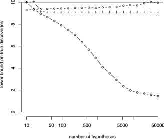
Figure 1: Simulation study as in Figure 1(b) in Meinshausen’s discussion, but with Simes’ local tests added. Meinshausen’s method (circles), Fisher combinations (diamonds) and Simes (plusses).

Depending on the alternative that is to be picked up, and depending on the type of statements that are to be made, different choices of local tests may lead to procedures with good or bad power. Obviously, this gives much room for the development of powerful procedures tailored to specific research questions on specific types of data.

2 Restricted Combinations

Westfall raises the important issue of restricted combinations. Restricted combinations occur when, because of logical relationships between hypotheses, the collection $T$ of true null hypotheses is a priori restricted, and some elements of the closure cannot be equal to the true set. In the example given by Westfall, the hypotheses are $H_{1}\dvtx\mu_{1}=\mu_{2}$, $H_{2}\dvtx\mu_{1}=\mu_{3}$ and $H_{3}\dvtx\mu_{2}=\mu_{3}$. For these hypotheses, $T=\{1,2\}$ is not possible, as simultaneous truth of $H_{1}$ and $H_{2}$ implies truth of $H_{3}$. Similarly, any other set $T$ of cardinality 2 is excluded, and $T$ can only take the values $\varnothing$, $\{1\}$, $\{2\}$, $\{3\}$ or $\{1,2,3\}$. We call those sets that cannot be equal to $T$ incongruent. There is an immense body of literature on multiple testing in the presence of restricted combinations, starting with the famous paper of Shaffer (1986), but we did not consider this issue in our paper.

Westfall claims that the method we have proposed may be conservative if restricted combinations are present. This is true. However, a very simple extension of the method can remove this conservativeness in a general way, which is very similar to Westfall’s treatment of the specific example. This extension follows from the Sequential Rejection Principle (Goeman and Solari, 2010). Applied to closed testing, this principle states that the local test of each $H_{I}$, $I\in\mathcal{C}$, when it is its turn to be tested, may assume that all hypotheses $H_{J}$, $J\supset I$ are false. For an incongruent set $I$, falsehood of all such hypotheses $H_{J}$ immediately implies that $H_{I}$ itself is false. Therefore, even the test that always rejects is a valid local test for the incongruent set $I$. Consequently, in the presence of restricted combinations, we may assume that the local test always rejects all incongruent sets.

The same conclusion may also be arrived at in an alternative way, by using the partitioning principle (Finner and Strassburger, 2002) rather than closed testing to make the confidence sets. For each $I\in\mathcal{C}$, let the corresponding partitioning hypothesis be

$$J_{I}=\bigcap_{i\in I}H_{i}\setminus\bigcup_{j\notin I}H_{j}.$$ (1)

Suppose an $\alpha$-level test is available for every $J_{I}$, $I\in\mathcal{C}$, and let $\mathcal{V}\subseteq\mathcal{C}$ be the index set of the partitioning hypotheses rejected by their corresponding test. Then, analogously to the closed testing based procedure, by the partitioning principle the intersection hypothesis $H_{I}$, $I\in\mathcal{C}$, is rejected whenever $J\in\mathcal{V}$ for every $J\supseteq I$. From this, we can make the set $\mathcal{X}$ of rejected intersection hypotheses and derive the upper confidence limit $t_{\alpha}(R)$ as before. The whole procedure is completely analogous to the one presented in the paper, only the smaller partitioning hypotheses $J_{I}$, $I\in\mathcal{C}$, take the role of the closure hypotheses $H_{I}$ when finding the set $\mathcal{X}$. As $J_{I}\subseteq H_{I}$, for every $I$, any valid test of $H_{I}$ is also a valid test for $J_{I}$, but $J_{I}=\varnothing$ for every incongruent $I$, so that we can safely reject every incongruent $J_{I}$. Consequently, again, we may assume that incongruent hypotheses are always rejected by their local test.

If we extend our method in this way, we have a general solution for the problem of restricted combinations. Using this extension, the conservativeness noted in Westfall’s example disappears, and the stronger statements he obtained are recovered. For concrete examples of families with restricted combinations, finding good shortcuts that take restricted combinations into account may, of course, still be a challenging problem.

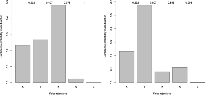
Figure 2: Confidence probability mass function for $R=\{$waist, forearm, calf, thigh} (left-hand side) and $R=\{$waist, forearm, height, thigh} (right-hand side). Cumulative percentages are given at the top of the figure.

3 Adjusted $p$-Values

The adjusted $p$-value is an important feature of multiple testing procedures, that conveys valuable additional information over the simple decision to reject or not to reject, as Westfall rightly points out. We did not go into the issue of adjusted $p$-values in the paper because we wanted to stress the analogy with confidence intervals, which are typically calculated for a fixed $\alpha$. It is possible, however, to find an analogy to adjusted $p$-value that conveys the same type of additional information, or even more.

By definition, an adjusted $p$-value of a certain hypothesis is the smallest $\alpha$-level that allows rejection of that hypothesis. By giving the threshold level $\alpha$ that distinguishes those $\alpha$-levels for which the hypothesis would or would not be rejected, the adjusted $p$-value gives the information what inferences would have been obtained if some other value of $\alpha$ would have been chosen. Analogously, in the exploratory setting, we may also vary the value of $\alpha$ and plot the upper confidence bound $t_{\alpha}(R)$ of the number of true hypotheses $\tau(R)$ as a function of $\alpha$. Just like the adjusted $p$-value, this shows the dependence of our conclusions on the arbitrary choice of $\alpha$.

An intuitive way to visualize the dependenceof $t_{\alpha}(R)$ on $\alpha$ is through a plot analogous to a confidence distribution (Singh, Xie and Strawderman, 2007). This can be obtained by interpreting the plot of $t_{\alpha}(R)$ as a function of $\alpha$ as if it was the quantile function of some discrete probability distribution, and plotting the differential of that, that is, the associated “probability mass function.” For the sets $R=$ {waist, forearm, calf, thigh} and $R=$ {waist, forearm, height, thigh} in the example of the physical data of Section 3 in the paper, this plot is given in Figure 2. From this plot, we can read off the 95% confidence limit $t_{0.95}(R)$ and the estimate $t_{1/2}(R)$ by finding the 95th quantile and the median, respectively. We can also read off the familywise error adjusted $p$-value at 1 minus the confidence distribution at 0.

It is important to realize that a confidence distribution is a random variable, not a probability distribution, in the same way that an adjusted $p$-value is a random variable, not a probability. The representation as if it was a distribution should just be seen as a convenient way to visualize the dependence of $t_{\alpha}(R)$ on $\alpha$. It is the direct analogue of the adjusted $p$-value for the method we have proposed.

4 The Practice of Exploratory Research

The methods we have presented still require a quite formal and planned design in which hypotheses have been formulated before data analysis and tests for intersection hypotheses are chosen beforehand. Such a way of working is close enough to actual data analysis in many genomics experiments, but it is far too formal to capture the great variety and freedom of true exploratory research. In actual practice, researchers often first perform a goodness-of-fit test on the same data before deciding what test to do. Researchers typically do additional unplanned hypotheses tests to detect the presence of effects suggested by plots of the same data. Also, researchers sometimes perform additional tests as a consequence of the nonsignificance of other test, because they are not satisfied with the non-significant result obtained. It is impossible to capture the true complexity of exploratory research in any formal method.

Heller suggests a two-stage approach that separates the data used for exploratory analysis in two parts. The first part is used as a pilot merely to decide what an appropriate model would be, and how intersection hypotheses should be tested, in a completely free exploratory manner. The end result of this data analysis would be a list of hypotheses and a plan for the closed testing procedure to be used in the next exploratory phase, which is then formal enough to allow use of the methods we have proposed. This proposal is practical and elegantly simple, mimicking the data splitting between exploratory and confirmatory research. It is also good that it stresses the need for a pilot experiment, which can be useful in many other respects as well. A practical problem, however, may be that many crucial decisions, regarding, for example, which test can be expected to have most power or which model fits best, may require quite large sample size, so that relatively small pilot experiments may not be adequate. One can also object philosophically to the idea, saying that the same arguments that can be used to change the empirical cycle from a two-phase process into a three-phase one could again be used to add a new fourth initial phase to the cycle, because the methods used in the pilot phase may be wrong or lacking in power. This way there would be no end to data splitting.

In the end, we think exploratory research in its most general form is too fluid to be captured in formal methodology. We feel, however, that we have demonstrated that more things are possible in the exploratory context than was commonly thought, and we hope we have stimulated the discussion on multiple testing in exploratory research. In our turn, we have been greatly stimulated by the contributions of the three discussants, for which we are thankful.

References

- (1) {barticle}[mr] \bauthor\bsnmBenjamini, \bfnmYoav\binitsY. and \bauthor\bsnmHeller, \bfnmRuth\binitsR. (\byear2008). \btitleScreening for partial conjunction hypotheses. \bjournalBiometrics \bvolume64 \bpages1215–1222. \biddoi=10.1111/j.1541-0420.2007.00984.x, issn=0006-341X, mr=2522270 \bptokimsref \endbibitem
- (2) {barticle}[mr] \bauthor\bsnmFinner, \bfnmH.\binitsH. and \bauthor\bsnmStrassburger, \bfnmK.\binitsK. (\byear2002). \btitleThe partitioning principle: A powerful tool in multiple decision theory. \bjournalAnn. Statist. \bvolume30 \bpages1194–1213. \biddoi=10.1214/aos/1031689023, issn=0090-5364, mr=1926174 \bptokimsref \endbibitem
- (3) {barticle}[mr] \bauthor\bsnmGoeman, \bfnmJelle J.\binitsJ. J. and \bauthor\bsnmSolari, \bfnmAldo\binitsA. (\byear2010). \btitleThe sequential rejection principle of familywise error control. \bjournalAnn. Statist. \bvolume38 \bpages3782–3810. \biddoi=10.1214/10-AOS829, issn=0090-5364, mr=2766868 \bptokimsref \endbibitem
- (4) {barticle}[author] \bauthor\bsnmGolub, \bfnmT. R.\binitsT. R., \bauthor\bsnmSlonim, \bfnmD. K.\binitsD. K., \bauthor\bsnmTamayo, \bfnmP.\binitsP., \bauthor\bsnmHuard, \bfnmC.\binitsC., \bauthor\bsnmGaasenbeek, \bfnmM.\binitsM., \bauthor\bsnmMesirov, \bfnmJ. P.\binitsJ. P., \bauthor\bsnmColler, \bfnmH.\binitsH., \bauthor\bsnmLoh, \bfnmM. L.\binitsM. L., \bauthor\bsnmDowning, \bfnmJ. R.\binitsJ. R., \bauthor\bsnmCaligiuri, \bfnmM. A.\binitsM. A. \betalet al. (\byear1999). \btitleMolecular classification of cancer: Class discovery and class prediction by gene expression monitoring. \bjournalScience \bvolume286 \bpages531–537. \bptokimsref \endbibitem
- (5) {barticle}[mr] \bauthor\bsnmHolm, \bfnmSture\binitsS. (\byear1979). \btitleA simple sequentially rejective multiple test procedure. \bjournalScand. J. Statist. \bvolume6 \bpages65–70. \bidissn=0303-6898, mr=0538597 \bptokimsref \endbibitem
- (6) {barticle}[mr] \bauthor\bsnmMeinshausen, \bfnmNicolai\binitsN. (\byear2006). \btitleFalse discovery control for multiple tests of association under general dependence. \bjournalScand. J. Statist. \bvolume33 \bpages227–237. \biddoi=10.1111/j.1467-9469.2005.00488.x, issn=0303-6898, mr=2279639 \bptokimsref \endbibitem
- (7) {barticle}[author] \bauthor\bsnmShaffer, \bfnmJ. P.\binitsJ. P. (\byear1986). \btitleModified sequentially rejective multiple test procedures. \bjournalJ. Amer. Statist. Assoc. \bvolume81 \bpages826–831. \bptokimsref \endbibitem
- (8) {bincollection}[mr] \bauthor\bsnmSingh, \bfnmKesar\binitsK., \bauthor\bsnmXie, \bfnmMinge\binitsM. and \bauthor\bsnmStrawderman, \bfnmWilliam E.\binitsW. E. (\byear2007). \btitleConfidence distribution (CD)—distribution estimator of a parameter. In \bbooktitleComplex Datasets and Inverse Problems. \bseriesInstitute of Mathematical Statistics Lecture Notes—Monograph Series \bvolume54 \bpages132–150. \bpublisherIMS, \baddressBeachwood, OH. \biddoi=10.1214/074921707000000102, mr=2459184 \bptokimsref \endbibitem