Critical behaviour of the randomly stirred dynamical Potts model: Novel universality class and effects of compressibility

Abstract

Critical behaviour of a nearly critical system, subjected to vivid turbulent mixing, is studied by means of the field theoretic renormalization group. Namely, relaxational stochastic dynamics of a non-conserved order parameter of the Ashkin-Teller-Potts model, coupled to a random velocity field with prescribed statistics, is considered. The mixing is modelled by Kraichnan’s rapid-change ensemble: time-decorrelated Gaussian velocity field with the power-like spectrum $\propto k^{-d-\xi}$. It is shown that, depending on the symmetry group of the underlying Potts model, the degree of compressibility and the relation between the exponent $\xi$ and the space dimension $d$, the system exhibits various types of infrared (long-time, large-scale) scaling behaviour, associated with four different infrared attractors of the renormalization group equations. In addition to known asymptotic regimes (equilibrium dynamics of the Potts model and the passively advected scalar field), existence of a new, strongly non-equilibrium type of critical behaviour is established. That “full-scale” regime corresponds to the novel type of critical behaviour (universality class), where the self-interaction of the order parameter and the turbulent mixing are equally important. The corresponding critical dimensions depend on $d$, $\xi$, the symmetry group and the degree of compressibility. The dimensions and the regions of stability for all the regimes are calculated in the leading order of the double expansion in two parameters $\xi$ and $\varepsilon=6-d$. Special attention is paid to the effects of compressibility of the fluid, because they lead to nontrivial qualitative crossover phenomena.

1 Introduction

Numerous complex systems, involving “infinitely” many degrees of freedom, demonstrate very interesting behaviour in the vicinity of their critical points. The typical feature of such systems is the divergence of the correlation length, although the underlying microscopic interactions are short-range ones. As a result, the behaviour of such systems “decouples” from their specific physical nature (fluids, magnets, superconductors etc.) and becomes highly universal: their thermodynamic and correlation functions exhibit scaling (self-similar) behaviour and depend only on “global” characteristics of the system (like its symmetry and dimension). Thus one can speak about the theory of critical state (or critical behaviour), in contradistinction with the numerous special theories of diverse critical phenomena (of course, very interesting and important on their own).

The adequate theory of critical state (both qualitative and quantitative) is based on the field theoretic renormalization group (RG); see the monographs [1, 2] for the detailed presentation and the bibliography. In the RG approach, possible types of critical behaviour (universality classes) are associated with infrared (IR) attractive fixed points of certain renormalizable field theoretic models.

Most typical equilibrium phase transitions belong to the universality class of the $O(n)$-symmetric $\psi^{4}$ model of an $n$-component scalar order parameter $\psi$. Universal characteristics of the critical behaviour (critical exponents, amplitude ratios, scaling functions) depend only on $n$ and on the spatial dimension $d$ and can be calculated within systematic perturbative schemes, in particular, in the form of expansions in $\varepsilon=4-d$, the deviation of the space dimension from its upper critical value $d=4$.

More exotic, but still actual and important example is provided by the Ashkin–Teller–Potts (or simply Potts) class of models [3]–[9]. In rough words, such a model describes a certain system which locally has $n$ states, while the energy of any given global configuration depends on whether the pairs of neighboring sites are in the same state or not. In the continuous formulation, Potts-type models are conveniently represented by the effective Hamiltonian for the $n$-component order parameter with a trilinear interaction term, invariant under the $n$-dimensional hypertetrahedron symmetry group [5]–[9].

The Potts-type models have numerous physical applications: solids and magnetic materials with nontrivial symmetry, spin glasses, nematic-to-isotropic transitions in the liquid crystals, bond percolation problem, random resistor networks and many others, see the papers [5]–[9] and the references therein. The Potts model (especially its paradigmatic special case $n=d=2$, the famous two-dimensional Ising model) has long become a source of inspiration for the new physical and mathematical ideas like integrability, conformal invariance, discrete holomorphisity etc.; for a recent discussion, see the papers [10], materials of the meeting [11] and references therein.

The problem of the nature of the phase transition in the Potts model has a long and entangled history; see e.g. the discussion in [8]. According to naively applied Landau’s phenomenological approach, existence of a triple term excludes the possibility of the second-order transition. On the contrary, exact two-dimensional results, numerical simulations and RG analysis suggest that for $n$ small enough, the phase transition in the Potts models is of the second order. We will not try to shed new light onto this interesting but difficult question: it should first be solved for the original static problem. To proceed, in this paper we accept the point of view that the existence of an IR attractive fixed point of the RG equations implies existence of a certain scaling (self-similar) IR asymptotic regime and, therefore, the existence of some kind of critical state.

It has long been realized that the behaviour of a real system near its critical point is extremely sensitive to external disturbances, gravity, geometry of the experimental setup, inclusion of impurities and so on; see the nice book [12] for the general discussion and references. The ideal critical behaviour of a pure equilibrium infinite system can be distorted by finite-size effects, limited accuracy of measuring the temperature, finite time of evolution (ageing) etc. What is more, some disturbances (randomly distributed impurities in magnets and turbulent mixing of fluid systems) can change the very type of the phase transition (first-order to second order one, and vice versa) and produce novel types of critical behaviour (universality classes) with rich and rather unexpected properties.

Investigation of the effects of various kinds of deterministic or chaotic flows on the behaviour of the critical fluids (like liquid crystals or binary mixtures) has shown that the flow can destroy the usual critical behaviour: it can change to the mean-field behaviour or, under some conditions, to a more complex behaviour described by new non-equilibrium universality classes [13]–[22].

In this paper we apply the field theoretic RG to study the effects of turbulent mixing on the critical behaviour of the (generalized) Potts model. Special attention will be paid to compressibility of the fluid, because it can lead to interesting crossover phenomena.

Bearing in mind applications to liquid crystals or percolation in moving media, we consider a purely relaxational stochastic dynamics of a non-conserved order parameter, coupled to a random velocity field.

The latter is modelled by the Kraichnan’s rapid-change ensemble: time-decorrelated Gaussian field with the pair correlation function of the form $\langle vv\rangle\propto\delta(t-t^{\prime})\,k^{-d-\xi}$, where $k$ is the wave number and $0<\xi<2$ is a free parameter with the most realistic (“Kolmogorov”) value $\xi=4/3$. Some time ago, the models involving passive scalar fields advected by such “synthetic” velocity ensembles attracted a great deal of attention because of the insight they offer into the origin of intermittency and anomalous scaling in the real fluid turbulence; see the review paper [23] and references therein. The RG approach to the problem of passive advection is reviewed in [24].

In the context of our study it is especially important that Kraichnan’s ensemble allows one to easily model compressibility of the fluid, which appears rather difficult if the velocity is modelled by dynamical equations; cf. [21].

The outline of the paper is the following. In section 2 we give the detailed description of the model and its field theoretic formulation. Following [9], we consider the generalized model with a certain symmetry group ${\cal G}$; the plain Potts model corresponds to the group $Z_{n}$. In section 3 we analyze the ultraviolet (UV) divergences and show that the model is multiplicatively renormalizable. Thus the RG equations are derived in the standard fashion; see section 4. The corresponding RG functions ($\beta$ functions and anomalous dimensions $\gamma$) are calculated in the one-loop approximation.

In section 5 we show that the model reveals four different types of critical behaviour, associated with four possible fixed points (strictly speaking, attractors of a more general form) of the corresponding RG equations. Three regimes correspond to known situations: Gaussian or free field theory, passively advected scalar field without self-interaction (the nonlinearity in the original stochastic equation is irrelevant), and the original Potts model without mixing. The most interesting fourth regime corresponds to a novel non-equilibrium universality class, formed by the interplay between the self-interaction and turbulent mixing.

A given critical regime can realize if the corresponding fixed point is admissible from the physics viewpoints: it should be IR attractive and lie in the physical range of model parameters. In our problem, admissibility of the fixed points depends on the spatial dimension $d$, exponent $\xi$, symmetry group ${\cal G}$ and the degree of compressibility. The regions of admissibility form a pattern in the space of model parameters, much more complicated in comparison with the $\psi^{4}$ model in the same velocity ensemble [21] or the Potts model in a strongly anisotropic shear flow [22]. As a result, interesting crossover phenomena occur as the degree of compressibility is varied. These issues are discussed in great detail in the same section 5.

In general, the critical dimensions in our problem are calculated as double series in $\varepsilon=6-d$ and $\xi$. In section 6 we present the explicit first-order (one-loop) expressions for the critical dimensions of the basic fields and parameters. Section 7 is reserved for a brief conclusion.

2 Description of the model. Field theoretic formulation

Relaxational dynamics of a non-conserved $n$-component order parameter $\psi_{a}(x)$ with $x\equiv\{t,\textbf{x}\}$ is described by the Langevin-type stochastic differential equation

$$\partial_{t}\psi_{a}(x)=-\lambda_{0}\,\frac{\delta{\cal H}(\psi)}{\delta\psi_{a}({\bf x})}\Bigg{|}_{{\bf x}\to x}+\zeta_{a}(x),$$ (2.1)

where $\partial_{t}=\partial/\partial{t}$, $\lambda_{0}>0$ is the (constant) kinetic coefficient and $\zeta_{a}(x)$ is a Gaussian random noise with zero average and the pair correlation function

$$\langle\zeta_{a}(x)\zeta_{b}(x^{\prime})\rangle=2\lambda_{0}\,\delta_{ab}\,\delta(t-t^{\prime})\,\delta^{(d)}(\bf x-\bf x^{\prime}),$$ (2.2)

where $d$ is the dimension of the $\bf x$ space. Here and below, the bare (unrenormalized) parameters are marked by the subscript “0.” Their renormalized counterparts (without the subscript) will appear later on. The normalization in (2.2) is chosen such that the steady-state equal-time correlation functions of the stochastic problem are given by the Boltzmann weight $\exp\{-{\cal H}(\psi)\}$.

Near the critical point, the static Hamiltonian ${\cal H}(\psi)$ of the Potts model is taken in the form [5, 6, 7]

$${\cal H}(\psi) = \int d{\bf x}\left\{-\frac{1}{2}\,\psi_{a}({\bf x})\partial^{2}\psi_{a}({\bf x})+\frac{\tau_{0}}{2}\,\psi_{a}({\bf x})\psi_{a}({\bf x})+\right.$$ (2.3)

$$+ \left.\frac{g_{0}}{3!}R_{abc}\,\psi_{a}({\bf x})\psi_{b}({\bf x})\psi_{c}({\bf x})\right\},$$

where $\partial_{i}=\partial/\partial x_{i}$ is the spatial derivative, $\partial^{2}=\partial_{i}\partial_{i}$ is the Laplace operator, $\tau_{0}\propto(T-T_{c})$ measures deviation of the temperature (or its analog) from the critical value and $g_{0}$ is the coupling constant. Summations over repeated indices are always implied ($a,b,c=1,\dots,n$ and $i=1,\dots,d$). After taking the functional derivative $\delta{\cal H}(\psi)/\psi({\bf x})$ one has to replace $\psi({\bf x})$ in (2.1) by the time-dependent field $\psi(x)$.

Following [9], we consider the generalized case of certain symmetry group ${\cal G}$, which has the only irreducible invariant third-rank tensor $R_{abc}$; without loss of generality it is assumed to be symmetric. In the one-loop approximation we will only need to know the coefficients $R_{1,2}$ in the contractions

$$R_{abc}R_{abe}=R_{1}\delta_{ce},\quad R_{aec}R_{chb}R_{b\!f\!a}=R_{2}R_{eh\!f}.$$ (2.4)

In the original Potts model ${\cal G}=Z_{n}$, the symmetry group of the hypertetrahedron in the $n$-dimensional space. Then it is convenient to express the tensor $R_{abc}$ in terms of the set of $(n+1)$ vectors $e^{\alpha}$ which define its vertices [5, 6]:

$$R_{abc}=\sum_{\alpha}e^{\alpha}_{a}e^{\alpha}_{b}e^{\alpha}_{c},$$

where the $e^{\alpha}_{a}$ satisfy

$$\sum_{\alpha=1}^{n+1}e^{\alpha}_{a}=0,\quad\sum_{\alpha=1}^{n+1}e^{\alpha}_{a}e^{\alpha}_{b}=(n+1)\delta_{ab},\quad\sum_{a=1}^{n}e^{\alpha}_{a}e^{\beta}_{a}=(n+1)\delta^{\alpha\beta}-1.$$ (2.5)

For the coefficients in (2.4) the relations (2.5) give

$$R_{1}=(n+1)^{2}(n-1),\quad R_{2}=(n+1)^{2}(n-2).$$ (2.6)

The stochastic problem (2.1), (2.2) can be reformulated as the field theoretic model of the doubled set of fields $\Phi=\{\psi,\psi^{{\dagger}}\}$ with the action functional

$${\cal S}(\psi,\psi^{{\dagger}})=\lambda_{0}\psi_{a}^{\dagger}\psi_{a}^{\dagger}\!+\!\psi_{a}^{{\dagger}}\left(-\partial_{t}+\lambda_{0}\partial^{2}\!-\!\lambda_{0}\tau_{0}\right)\psi_{a}\!-\!g_{0}\lambda_{0}R_{abc}\psi^{{\dagger}}_{a}\psi_{b}\psi_{c}/2.$$ (2.7)

Here $\psi^{{\dagger}}=\psi^{{\dagger}}(t,{\bf x})$ is an auxiliary “response field” and all the needed integrations over the arguments of the fields and summations over the repeated indices are implied, for example

$$\psi_{a}^{{\dagger}}\partial_{t}\psi_{a}=\sum_{a=1}^{n}\int dt\int d{\bf x}\psi_{a}^{{\dagger}}(t,{\bf x})\partial_{t}\psi_{a}(t,{\bf x}).$$

This formulation means that the statistical averages of the random quantities in the original stochastic problem can be represented by functional integrals over the full set of fields with the weight $\exp{\cal S}(\Phi)$, and can therefore be interpreted as the Green functions of the field theoretic model with the action (2.7).

The model (2.7) corresponds to the standard Feynman diagrammatic technique with two bare propagators $\langle\psi\psi^{{\dagger}}\rangle_{0}$, $\langle\psi\psi\rangle_{0}$ and the trilinear vertex $\sim\psi^{\dagger}\psi^{2}$. In the frequency-momentum ($\omega$–${\bf k}$) representation the propagators have the forms

$$\langle\psi_{a}\psi_{b}^{{\dagger}}\rangle_{0}(\omega,{\bf k})=\frac{\delta_{ab}}{-{\rm i}\omega+\lambda_{0}\left(k^{2}+\tau_{0}\right)},$$

$$\langle\psi_{a}\psi_{b}\rangle_{0}(\omega,{\bf k})=\frac{2\lambda_{0}\delta_{ab}}{\omega^{2}+\lambda_{0}^{2}\left(k^{2}+\tau_{0}\right)^{2}},$$ (2.8)

where $k=|{\bf k}|$ is the wave number.

The Galilean invariant coupling with the velocity field ${\bf v}=\{v_{i}(t,{\bf x})\}$ for the compressible fluid ($\partial_{i}v_{i}\neq 0$) is introduced by the replacement

$$\partial_{t}\psi\to\partial_{t}\psi+a_{0}\,\partial_{i}(v_{i}\psi)+(a_{0}-1)(v_{i}\partial_{i})\psi=\nabla_{t}\psi+a_{0}(\partial_{i}v_{i})\psi$$ (2.9)

in (2.1). Here $\nabla_{t}\equiv\partial_{t}+v_{i}\partial_{i}$ is the Galilean covariant (Lagrangian) derivative and $a_{0}$ is an arbitrary parameter. For the linear advection-diffusion equation, the choice $a_{0}=1$ corresponds to the conserved quantity $\psi$ (e.g. density of an impurity) while $a_{0}=0$ is referred to as “tracer” (concentration of the impurity or the temperature of the fluid; in this case, the conserved quantity is $\psi^{{\dagger}}$). In the presence of a nonlinearity in (2.1), it is necessary to keep all the terms in (2.9) in order to ensure multiplicative renormalizability [21].

In the real problem, the field ${\bf v}(t,{\bf x})$ is governed by the Navier–Stokes equation. Here we employ a simplified rapid-change model, in which the velocity obeys a Gaussian statistics with zero average and the prescribed correlation function

$$\langle v_{i}(t,{\bf x})v_{j}(t^{\prime},{\bf x^{\prime}})\rangle=\delta(t-t^{\prime})\,D_{ij}({\bf r}),\quad{\bf r}={\bf x}-{\bf x^{\prime}}$$ (2.10)

with

$$D_{ij}({\bf r})=D_{0}\,\int_{k>m}\frac{d{\bf k}}{(2\pi)^{d}}\,\frac{1}{k^{d+\xi}}\,\left\{P_{ij}({\bf k})+\alpha Q_{ij}({\bf k})\right\}\,\exp({\rm i}{\bf kr}).$$ (2.11)

Here $P_{ij}({\bf k})=\delta_{ij}-k_{i}k_{j}/k^{2}$ and $Q_{ij}({\bf k})=k_{i}k_{j}/k^{2}$ are the transverse and the longitudinal projectors, respectively, $D_{0}>0$ is an amplitude factor and $\alpha\geq 0$ is an arbitrary parameter which measures the degree of compressibility. The case $\alpha=0$ corresponds to the incompressible fluid ($\partial_{i}v_{i}=0$), while the limit $\alpha\to\infty$ at fixed $\alpha D_{0}$ corresponds to the purely potential velocity field. The exponent $0<\xi<2$ is a free parameter which can be viewed as a kind of Hölder exponent, which measures “roughness” of the velocity field; its “Kolmogorov” value is $\xi=4/3$, while the “Batchelor” limit $\xi\to 2$ corresponds to smooth velocity. The cutoff in the integral (2.11) from below at $k=m$, where $m\equiv 1/{\cal L}$ is the reciprocal of the integral turbulence scale ${\cal L}$, provides IR regularization. Its precise form is inessential; the sharp cutoff is the simplest choice from calculational viewpoints.

The action functional for the full set of fields $\Phi=\left\{\psi,\psi^{{\dagger}},{\bf v}\right\}$ becomes

$${\cal S}(\Phi) = \lambda_{0}\psi^{{\dagger}}_{a}\psi^{{\dagger}}_{a}+\psi^{{\dagger}}_{a}\left\{-\nabla_{t}+\lambda_{0}\left(\partial^{2}-\tau_{0}\right)-a_{0}(\partial_{i}v_{i})\right\}\psi_{a}+$$ (2.12)

$$- \frac{g_{0}\lambda_{0}}{2}R_{abc}\psi^{{\dagger}}_{a}\psi_{b}\psi_{c}+{\cal S}_{v}({\bf v}).$$

It is obtained from (2.7) by the substitution (2.9) and adding the term corresponding to the Gaussian averaging over the velocity field with the correlator (2.10), (2.11):

$${\cal S}_{v}({\bf v})=-\frac{1}{2}\int dt\int d{\bf x}\int d{\bf x^{\prime}}v_{i}(t,{\bf x})D_{ij}^{-1}({\bf r})v_{j}(t,{\bf x^{\prime}}),$$ (2.13)

where $D_{ij}^{-1}({\bf r})\propto D_{0}^{-1}r^{-2d-\xi}$ with $r=|{\bf r}|$ is the kernel of the linear operation inverse to $D_{ij}({\bf r})$ from (2.11).

In addition to (2.8), the diagrammatic technique for the full-scale model involves the velocity propagator $\langle vv\rangle_{0}$ defined by the relations (2.10), (2.11) and the new vertex

$$\psi_{a}^{{\dagger}}v_{i}V_{i,ab}\psi_{b}\equiv-\psi_{a}^{{\dagger}}\left\{(v_{i}\partial_{i})\psi_{a}+a_{0}(\partial_{i}v_{i})\psi_{a}\right\}$$ (2.14)

with the vertex factor

$$V_{i,ab}=-{\rm i}\delta_{ab}(k_{i}+a_{0}q_{i}),$$ (2.15)

where $q_{i}$ is the momentum argument of $v_{i}$ and $k_{i}$ is the momentum of the field $\psi$.

As usual for a trilinear interaction, the actual expansion parameter in the model (2.7) is $u_{0}\equiv g_{0}^{2}$ rather than $g_{0}$ itself. Thus for the full model (2.12) the part of the coupling constants (expansion parameters in the ordinary perturbation theory) is played by the three parameters

$$u_{0}=g_{0}^{2}\sim\Lambda^{6-d},\quad w_{0}=D_{0}/\lambda_{0}\sim\Lambda^{\xi},\quad w_{0}a_{0}\sim\Lambda^{\xi}.$$ (2.16)

The last relations follow from the dimensionality considerations (more precisely, see the next section) and set in the characteristic UV momentum scale $\Lambda$. The first relation in (2.16) shows that the interaction $\psi^{\dagger}\psi^{2}$ becomes logarithmic (the corresponding coupling constant $u_{0}$ becomes dimensionless) for $d=6$. Thus for the single-charge problem (2.7) the value $d=6$ is the upper critical dimension, and the deviation $\varepsilon=6-d$ plays the role of the expansion parameter in the RG approach: the critical dimensions are nontrivial for $\varepsilon>0$ and can be calculated in the form of series in $\varepsilon$.

The additional interaction (2.14) of the full model becomes logarithmic for $\xi=0$. The parameter $\xi$ is not related to the spatial dimension and can be varied independently. For the RG analysis of the full-scale problem it is important that all the interactions become logarithmic simultaneously. Otherwise, one of them would be weaker than the other from the RG viewpoint and it would be irrelevant in the leading-order IR behaviour. As a result, some of the scaling regimes of the full model would be lost. In order to study all possible scaling regimes and the crossovers between them, we need a genuine multicharge theory, in which all the interactions are treated on equal footing. Thus in the following we treat $\varepsilon$ and $\xi$ as small parameters of the same order, $\varepsilon\propto\xi$. Instead of the ordinary $\varepsilon$ expansion in the single-charge models, the coordinates of the fixed points, critical dimensions and other quantities will be calculated as double expansions in $\varepsilon$ and $\xi$.

3 Canonical dimensions, UV divergences and renormalization

It is well known that the analysis of UV divergences is based on the analysis of canonical dimensions (“power counting”); see e.g. [1, 2]. Dynamical models of the type (2.7), (2.12), in contrast to static ones, have two independent scales: the time scale $T$ and the length scale $L$. Thus the canonical dimension of any quantity $F$ (a field or a parameter) is described by two numbers, the momentum dimension $d_{F}^{k}$ and the frequency dimension $d_{F}^{\omega}$, defined such that $[F]\sim[L]^{-d_{F}^{k}}[T]^{-d_{F}^{\omega}}$. By definition

$$d_{k}^{k}=-d_{\bf x}^{k}=1,\ d_{k}^{\omega}=d_{\bf x}^{\omega}=0,\ d_{\omega}^{k}=d_{t}^{k}=0,\ d_{\omega}^{\omega}=-d_{t}^{\omega}=1,$$

while the other dimensions are found from the requirement that each term of the action functional be dimensionless (with respect to the momentum and frequency dimensions separately). Then, based on $d_{F}^{k}$ and $d_{F}^{\omega}$, one can introduce the total canonical dimension $d_{F}=d_{F}^{k}+2d_{F}^{\omega}$ (in the free theory, $\partial_{t}\propto\partial^{2}$), which plays in the theory of renormalization of dynamical models the same part as the conventional (momentum) dimension does in static problems; see e.g. chap. 5 of [2]. The canonical dimensions for the models (2.12) are given in table 1, including the renormalized parameters (without subscript “0”), which will be introduced shortly.

Table 1: Canonical dimensions of the fields and parameters in the model (2.12).

$F$	$\psi$	$\psi^{\dagger}$	$v$	$\lambda_{0},\lambda$	$\tau_{0},\tau$	$m,\mu,\Lambda$	$u_{0}$	$w_{0}$	$u,w,a_{0},a,\alpha$
$d_{F}^{k}$	$(d-2)/2$	$(d+2)/2$	$-1$	$-2$	$2$	$1$	$6-d$	$\xi$	$0$
$d_{F}^{\omega}$	0	0	$1$	$1$	$0$	$0$	$0$	$0$	$0$
$d_{F}$	$(d-2)/2$	$(d+2)/2$	$1$	$0$	$2$	$1$	$6-d$	$\xi$	$0$

As already discussed in the end of the preceding section, the full model (2.12) is logarithmic (all the coupling constants are simultaneously dimensionless) at $d=6$ and $\xi=0$. Thus the UV divergences in the Green functions manifest themselves as singularities in $\varepsilon=6-d$, $\xi$ and, in general, in their linear combinations.

The total canonical dimension of an arbitrary 1-irreducible Green function $\Gamma=\langle\Phi\cdots\Phi\rangle_{\rm 1-ir}$ is given by the relation [2]

$$d_{\Gamma}=d_{\Gamma}^{k}+2d_{\Gamma}^{\omega}=d+2-N_{\Phi}d_{\Phi},$$ (3.1)

where $N_{\Phi}=\{N_{\psi},N_{\psi^{{\dagger}}},N_{v}\}$ are the numbers of corresponding fields entering the function $\Gamma$, and the summation over all types of the fields is implied. The total dimension $d_{\Gamma}$ in the logarithmic theory (that is, at $\varepsilon=\xi=0$) is the formal index of the UV divergence $\delta_{\Gamma}=d_{\Gamma}|_{\varepsilon=\xi=0}$. Superficial UV divergences, whose removal requires counterterms, can appear only in the functions $\Gamma$ for which $\delta_{\Gamma}$ is a non-negative integer. From table 1 and (3.1) we find

$$\delta_{\Gamma}=8-2N_{\psi}-4N_{\psi^{{\dagger}}}-N_{v}.$$ (3.2)

Dimensional analysis should be augmented by certain additional considerations. In dynamical models of the type (2.12), all the 1-irreducible diagrams without the fields $\psi^{{\dagger}}$ vanish, and it is sufficient to consider the functions with $N_{\psi^{{\dagger}}}\geq 1$ [2]. Furthermore, an important role is played by the Galilean symmetry and the invariance with respect to the group ${\cal G}$. For example, the function $\left\langle\psi^{{\dagger}}\psi vv\right\rangle_{\rm 1-ir}$ can be omitted from consideration because the corresponding counterterm $\psi^{{\dagger}}_{a}\psi_{a}v^{2}$ is forbidden by the Galilean invariance. A similar situation occurs for the function $\left\langle\psi^{{\dagger}}vv\right\rangle_{\rm 1-ir}$: the possible counterterms $\psi^{{\dagger}}_{a}(\partial_{i}v_{k})(\partial_{k}v_{i})$ and $\psi^{{\dagger}}_{a}(\partial_{i}v_{k})(\partial_{i}v_{k})$ are forbidden by the symmetry with respect to ${\cal G}$. In turn, owing to the symmetry with respect to ${\cal G}$, the trilinear term in (2.12) is renormalized as a single entity.

With those restrictions, the analysis of the expression (3.2) shows that in our model, superficial UV divergences can only be present in the following 1-irreducible functions:

$$\langle\psi^{{\dagger}}\psi^{{\dagger}}\rangle_{\rm 1-ir}\quad(\delta=0)\quad{\rm with\ the\ counterterm}\quad\psi_{a}^{{\dagger}}\psi_{a}^{{\dagger}},$$

$$\langle\psi^{{\dagger}}\psi\rangle_{\rm 1-ir}\quad(\delta=2)\quad{\rm with\ the\ counterterms}\quad\psi_{a}^{{\dagger}}\partial_{t}\psi_{a},\ \psi_{a}^{{\dagger}}\partial^{2}\psi_{a},\ \psi_{a}^{{\dagger}}\psi_{a},$$

$$\langle\psi^{{\dagger}}\psi\psi\rangle_{\rm 1-ir}\quad(\delta=0)\quad{\rm with\ the\ counterterm}\quad R_{abc}\psi_{a}^{{\dagger}}\psi_{b}\psi_{c},$$

$$\langle\psi^{{\dagger}}\psi v\rangle_{\rm 1-ir}\quad(\delta=1)\quad{\rm with\ the\ counterterms}\quad\psi_{a}^{{\dagger}}(v_{i}\partial_{i})\psi_{a},\ \psi_{a}^{{\dagger}}(\partial_{i}v_{i})\psi_{a}.$$

All these terms are present in the action functional (2.12), so that our model appears multiplicatively renormalizable. The Galilean symmetry also requires that the counterterms $\psi^{{\dagger}}\partial_{t}\psi$ and $\psi^{{\dagger}}(v\partial)\psi$ enter the renormalized action only in the form of the Lagrangian derivative $\psi^{{\dagger}}\nabla_{t}\psi$, imposing no restriction on the Galilean invariant term $\psi^{{\dagger}}(\partial v)\psi$.

We thus conclude that the renormalized action can be written in the form

$${\cal S}_{R}(\Phi) = \psi^{{\dagger}}_{a}\left\{-Z_{1}\nabla_{t}+\lambda\left(Z_{2}\partial^{2}-Z_{3}\tau\right)-aZ_{6}(\partial_{i}v_{i})\right\}\psi_{a}+$$ (3.3)

$$+ \lambda Z_{5}\psi^{{\dagger}}_{a}\psi^{{\dagger}}_{a}-g\mu^{\varepsilon/2}R_{abc}\lambda Z_{4}\psi^{{\dagger}}_{a}\psi_{b}\psi_{c}/2+{\cal S}_{v}({\bf v})$$

with the same ${\cal S}_{v}({\bf v})$ from (2.13).

Here $\lambda$, $\tau$, $g$ and $a$ are renormalized counterparts of the bare parameters (with the subscripts “0”) and $\mu$ is the reference momentum scale (additional arbitrary parameter of the renormalized theory). The renormalization constants $Z$ absorb the singularities in $\varepsilon$ and $\xi$ and depend on the dimensionless parameters $u$, $w$, $a$ and $\alpha$. Expression (3.3) can be reproduced by the multiplicative renormalization of the fields $\psi\to\psi Z_{\psi}$, $\psi^{{\dagger}}\to\psi^{{\dagger}}Z_{\psi^{{\dagger}}}$ and the parameters:

$$g_{0} = g\mu^{\varepsilon/2}Z_{g},\quad u_{0}=u\mu^{\varepsilon}Z_{u},\quad w_{0}=w\mu^{\xi}Z_{w},$$

$$\lambda_{0} = \lambda Z_{\lambda},\quad\tau_{0}=\tau Z_{\tau},\quad a_{0}=aZ_{\tau}.$$ (3.4)

Since the last term ${\cal S}_{v}({\bf v})$ in (3.3) remains intact, the amplitude $D_{0}$ from (2.11) is expressed in renormalized parameters as $D_{0}=w_{0}\lambda_{0}=w\lambda\mu^{\xi}$, while the parameters $m$ and $\alpha$ are not renormalized: $m_{0}=m$, $\alpha_{0}=\alpha$. Owing to the Galilean symmetry, the both terms in the covariant derivative $\nabla_{t}$ are renormalized with the same constant $Z_{1}$, so that the velocity field is not renormalized, either. Hence the exact relations

$$Z_{w}Z_{\lambda}=1,\quad Z_{m}=Z_{\alpha}=Z_{v}=1.$$ (3.5)

Comparison of the expressions (2.12) and (3.3) gives the following relations between the renormalization constants $Z_{1}$–$Z_{6}$ and (3.4):

$$Z_{1} = Z_{\psi}Z_{\psi^{\dagger}},\quad Z_{2}=Z_{1}Z_{\lambda},\quad Z_{3}=Z_{2}Z_{\tau},$$

$$Z_{4} = Z_{\lambda}Z_{g}Z_{\psi}^{2}Z_{\psi^{\dagger}},\quad Z_{5}=Z_{\lambda}Z_{\psi^{\dagger}}^{2},\quad Z_{6}=Z_{1}Z_{a}.$$ (3.6)

Resolving these relations with respect to the renormalization constants of the fields and parameters gives

$$Z_{\lambda} = Z_{1}^{-1}Z_{2},\quad Z_{\tau}=Z_{2}^{-1}Z_{3},\quad Z_{a}=Z_{1}^{-1}Z_{6},\quad Z_{u}=Z_{1}^{-1}Z_{2}^{-3}Z_{4}^{2}Z_{5},$$

$$Z_{\psi} = Z_{1}^{1/2}Z_{2}^{1/2}Z_{5}^{-1/2},\quad Z_{\psi^{{\dagger}}}=Z_{1}^{1/2}Z_{2}^{-1/2}Z_{5}^{1/2},$$ (3.7)

where we have passed to the coupling constant $u=g^{2}$ with $Z_{u}=Z_{g}^{2}$.

The renormalization constants can be found from the requirement that the Green functions of the renormalized model (3.3), when expressed in renormalized variables, be UV finite (in our case, finite at $\varepsilon\to 0$, $\xi\to 0$). The constants $Z_{1}$–$Z_{6}$ are calculated directly from the diagrams, then the constants in (3.4) are found from (3.7). In order to find the full set of constants, it is sufficient to consider the 1-irreducible Green functions which involve superficial divergences. The diagrammatic representation for the relevant Green functions in the one-loop approximation is given on figure 1.

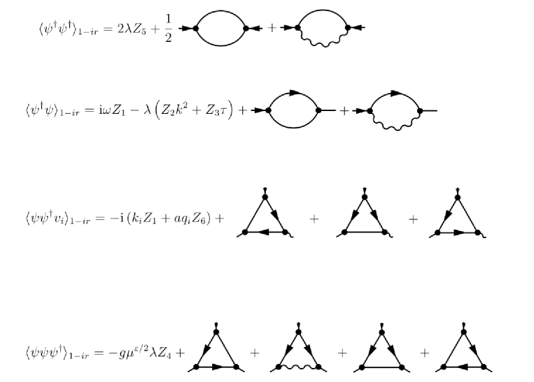
Figure 1: Superficially divergent 1-irreducible Green functions in the one-loop approximation.

The solid lines with arrows denote the propagator $\langle\psi\psi^{{\dagger}}\rangle_{0}$, the arrow pointing to the field $\psi^{{\dagger}}$. The solid lines without arrows correspond to the propagator $\langle\psi\psi\rangle_{0}$ and the wavy lines denote the velocity propagator $\langle vv\rangle_{0}$ defined in (2.10) and (2.11). The external ends with incoming arrows correspond to the fields $\psi^{{\dagger}}$, the ends without arrows correspond to $\psi$. The triple vertices with one wavy line correspond to the vertex factor (2.15). In order to calculate the renormalization constants, it is sufficient to consider the symmetric phase with $\tau>0$. Then, with respect to the “isovector” indices, all the terms in the first three lines on figure 1 are proportional to $\delta_{ab}$ while all the terms in last line are proportional to $R_{abc}$.

All the diagrammatic elements should be expressed in renormalized variables using the relations (3.4)–(3.6). In the one-loop approximation, the $Z$’s in the bare terms should be taken in the first order in $u=g^{2}$ and $w$, while in the diagrams they should simply be replaced with unities, $Z\to 1$. Thus the passage to renormalized variables in the diagrams is achieved by the simple substitutions $\lambda_{0}\to\lambda$, $\tau_{0}\to\tau$, $g_{0}\to g\mu^{\varepsilon/2}$ and $w_{0}\to w\mu^{\xi}$.

In practical calculations, we used the minimal subtraction (MS) scheme, where all the renormalization constants have the forms “$Z=1+\,$ only singularities in $\varepsilon$ and $\xi$,” with the coefficients depending on the completely dimensionless renormalized parameters $u$, $w$, $a$ and $\alpha$.

The one-loop calculations for similar models are discussed in detail, e.g., in [19]–[21], and here we only give the results:

$$Z_{1} = 1-\frac{uR_{1}}{2\varepsilon},\quad Z_{2}=1-\frac{uR_{1}}{3\varepsilon}-\frac{w}{6\xi}(5+\alpha),\quad Z_{3}=1-\frac{2R_{1}u}{\varepsilon},$$

$$Z_{4} = 1-\frac{2R_{2}u}{\varepsilon}-\frac{w\alpha a^{2}}{\xi},\quad Z_{5}=1-\frac{uR_{1}}{2\varepsilon}-\frac{w}{\xi}\alpha(a-1)^{2},$$

$$Z_{6} = 1-\frac{uR_{1}}{2a\varepsilon}(4a-1)$$ (3.8)

with $R_{1,2}$ from (2.4) and up to the corrections of the order $u^{2}$, $w^{2}$, $uw$ and higher. To simplify the resulting expressions, we have passed to the new parameters

$$u\to u/128\pi^{3},\quad w\to w/64\pi^{3};$$

in (3.8) and below they are denoted by the same symbols $u$ and $w$.

4 RG functions and equations

Let us briefly recall an elementary derivation of the RG equations; detailed presentation can be found e.g. in [1, 2]. The RG equations are written for the renormalized Green functions $W^{R}=\langle\Phi\cdots\Phi\rangle_{R}$, which differ from the original (unrenormalized) ones $W=\langle\Phi\cdots\Phi\rangle$ only by normalization (due to rescaling of the fields) and choice of parameters, and therefore can equally be used for analyzing the critical behaviour. The relation ${\cal S}_{R}(\Phi,e,\mu)={\cal S}(Z_{\Phi}\Phi,e_{0})$ between the bare (2.12) and renormalized (3.3) action functionals results in the relations

$$W(e_{0},\dots)=Z_{\psi}^{N_{\psi}}Z_{\psi^{\dagger}}^{N_{\psi^{\dagger}}}W^{R}(e,\mu,\dots).$$ (4.1)

between the Green functions. Here $N_{\psi}$ and $N_{\psi^{\dagger}}$ are the numbers of corresponding fields in the function $W$ (we recall that in our model $Z_{v}=1$); $e_{0}=\{\lambda_{0},\tau_{0},u_{0},w_{0},a_{0},m_{0},\alpha_{0}\}$ is the full set of bare parameters and $e=\{\lambda,\tau,u,w,a,m,\alpha\}$ are their renormalized analogs (we recall that $\alpha_{0}=\alpha$ and $m_{0}=m$); the ellipsis stands for the other arguments (coordinates/momenta or times/frequencies).

We use $\widetilde{\cal D}_{\mu}$ to denote the differential operation $\mu\partial_{\mu}$ for fixed $e_{0}$ and operate on both sides of the relation (4.1) with it. This gives the basic RG differential equation:

$$\left\{{\cal D}_{RG}+N_{\psi}\gamma_{\psi}+N_{\psi^{{\dagger}}}\gamma_{\psi^{{\dagger}}}\right\}\,W^{R}(e,\mu,\dots)=0,$$ (4.2)

where ${\cal D}_{RG}$ is the operation $\widetilde{\cal D}_{\mu}$ expressed in the renormalized variables:

$${\cal D}_{RG}\equiv{\cal D}_{\mu}+\beta_{u}\partial_{u}+\beta_{w}\partial_{w}+\beta_{a}\partial_{a}-\gamma_{\lambda}{\cal D}_{\lambda}-\gamma_{\tau}{\cal D}_{\tau}$$ (4.3)

and we have written ${\cal D}_{x}\equiv x\partial_{x}$ for any variable $x$. The anomalous dimensions $\gamma$ are defined as

$$\gamma_{F}\equiv\widetilde{\cal D}_{\mu}\ln Z_{F}\quad{\rm for\ any\ quantity}\ F,$$ (4.4)

while the $\beta$ functions for the coupling constants $u$, $w$ and $a$ are

$$\beta_{u}\equiv\widetilde{\cal D}_{\mu}u=u\,(-\varepsilon-\gamma_{u}),$$

$$\beta_{w}\equiv\widetilde{\cal D}_{\mu}w=w\,(-\xi-\gamma_{w}),$$

$$\beta_{a}\equiv\widetilde{\cal D}_{\mu}a=-a\gamma_{a},$$ (4.5)

where the second equalities come from the definitions and the relations (3.4). In principle, the dimensionless parameter $\alpha$ should be treated as the fourth coupling constant, but the corresponding $\beta$ function

$$\beta_{\alpha}=\widetilde{\cal D}_{\mu}\alpha=-\alpha\gamma_{\alpha}$$ (4.6)

vanishes identically due to (4.12) and does not appear in the subsequent relations.

The anomalous dimension corresponding to a given renormalization constant $Z_{F}$ is found from the relation

$$\gamma_{F}=\left(\beta_{u}\partial_{u}+\beta_{w}\partial_{w}+\beta_{a}\partial_{a}\right)\ln Z_{F}\simeq-\left(\varepsilon{\cal D}_{u}+\xi{\cal D}_{w}\right)\ln Z_{F}.$$ (4.7)

The first equality follows from the definition (4.4), expression (4.3) for the operation $\widetilde{\cal D}_{\mu}$ in renormalized variables, and the fact that the $Z$’s depend only on the completely dimensionless coupling constants $u$, $w$ and $a$. In the second (approximate) equality, we only retained the leading-order terms in the $\beta$ functions (4.5), which is sufficient for the first-order approximation. The leading-order expressions (3.8) for the renormalization constants have the forms

$$Z_{F}=1+\frac{u}{\varepsilon}{\cal A}_{F}(a,\alpha)+\frac{w}{\xi}{\cal B_{F}}(a,\alpha).$$ (4.8)

The factors $\varepsilon$ and $\xi$ in (4.7) cancel the corresponding poles contained in the expressions (4.8) for the constants $Z_{F}$, which leads to the final UV finite expressions for the anomalous dimensions:

$$\gamma_{F}=-u{\cal A}_{F}(a,\alpha)-w{\cal B}_{F}(a,\alpha)$$ (4.9)

for any constant $Z_{F}$. Then equations (3.8) give

$$\gamma_{1} = R_{1}u/2,\quad\gamma_{2}=R_{1}u/3+w(5+\alpha)/6,\quad\gamma_{3}=2R_{1}u,$$

$$\gamma_{4} = 2R_{2}u+w\alpha a^{2},\quad\gamma_{5}=uR_{1}/2+w\alpha(a-1)^{2},$$

$$\gamma_{6} = uR_{1}(4a-1)/2a.$$ (4.10)

The multiplicative relations (3.6) between the renormalization constants result in the linear relations between the corresponding anomalous dimensions:

$$\gamma_{\lambda} = \gamma_{2}-\gamma_{1},\quad\gamma_{\tau}=\gamma_{3}-\gamma_{2},$$

$$\gamma_{a} = \gamma_{6}-\gamma_{1},\quad\gamma_{u}=-\gamma_{1}-3\gamma_{2}+2\gamma_{4}+\gamma_{5},$$

$$2\gamma_{\psi} = \gamma_{1}+\gamma_{2}-\gamma_{5},\quad 2\gamma_{\psi^{{\dagger}}}=\gamma_{1}-\gamma_{2}+\gamma_{5},$$ (4.11)

while the exact relations (3.5) result in

$$\gamma_{w}=-\gamma_{\lambda},\quad\gamma_{m}=\gamma_{\alpha}=\gamma_{v}=0.$$ (4.12)

Along with (4.10), those relations give the final first-order explicit expressions for the anomalous dimensions of the fields and parameters:

$$\gamma_{\lambda} = -\gamma_{w}=-R_{1}u/6+w(5+\alpha)/6,\ \gamma_{\tau}=5R_{1}u/3-w(5+\alpha)/6,$$

$$\gamma_{u} = -uR-w(5+\alpha)/2+w\alpha f(a),\ \gamma_{a}=(3a-1)R_{1}u/2a,$$

$$2\gamma_{\psi} = R_{1}u/3-w\left[5w(\alpha-1)/6+\alpha a(a-2)\right],$$

$$2\gamma_{\psi^{{\dagger}}} = 2R_{1}u/3+w\left[5w(\alpha-1)/6+\alpha a(a-2)\right],$$ (4.13)

where we have denoted $R=R_{1}-4R_{2}$ and $f(a)=2a^{2}+(a-1)^{2}$.

5 Attractors of the RG equations and scaling regimes

It is well known that possible asymptotic regimes of a renormalizable field theoretic model are determined by the asymptotic behaviour of the system of ordinary differential equations for the so-called invariant (running) coupling constants

$${\cal D}_{s}\bar{g}_{i}(s,g)=\beta_{i}(\bar{g}),\quad\bar{g}_{i}(1,g)=g_{i},$$ (5.1)

where $s=k/\mu$, $g=\{g_{i}\}$ is the full set of couplings and $\bar{g}_{i}(s,g)$ are the corresponding invariant variables. As a rule, the IR ($s\to 0$) and UV ($s\to\infty$) behaviour of such system is determined by fixed points $g_{i*}$. The coordinates of possible fixed points are found from the requirement that all the $\beta$ functions vanish:

$$\beta_{i}(g_{*})=0.$$ (5.2)

The type of a given fixed point is determined by the matrix

$$\Omega_{ij}=\partial\beta_{i}/\partial g_{j}|_{g=g^{*}}\,,$$ (5.3)

which appears in the linearized version of the system (5.1) near that point. For IR attractive fixed points (which we are interested in here) the matrix $\Omega$ is positive, i.e. the real parts of all its eigenvalues are positive. In the case at hand, the fixed points for the full set of couplings $u$, $w$, $a$, $\alpha$ are determined by the equations

$$\beta_{u,w,a,\alpha}(u_{*},w_{*},a_{*},\alpha_{*})=0,$$ (5.4)

with the $\beta$ functions defined in the previous section. However, in our model the attractors of the system (5.1) involve, in general, two-dimensional surfaces in the full four-dimensional space of couplings. Indeed, the function (4.6) vanishes identically, and the equation $\beta_{\alpha}=0$ imposes no restriction on the parameter $\alpha$. Thus it is convenient to consider the attractors of the system (5.1) in the three-dimensional space $u$, $w$, $a$; their coordinates, matrix (5.3) and the critical exponents depend, in general, on the free parameter $\alpha$. Furthermore, in this reduced space some attractors will be not simply fixed points, but also lines of fixed points, parametrized by the coupling $a$. In the following we will use the term “fixed point” for all those attractors, bearing in mind that their coordinates can depend on $\alpha$ and, in general, on $a$.

The couplings $u_{*}$ and $w_{*}$ should be positive (by definition, $u\propto g^{2}>0$ and $w\propto D_{0}/\lambda>0$), so that the point is admissible from the physics viewpoints if it satisfies the conditions

$$u_{*}>0,\quad w_{*}>0$$ (5.5)

and can be IR attractive ($\Omega>0$) for some values of the model parameters (in fact, all the above inequalities can be non-strict).

In the one-loop approximation, the $\beta$ functions are found from the definitions (4.5) and the explicit expressions (4.12) and (4.13):

$$\beta_{u} = u\left[-\varepsilon+Ru+w(5+\alpha)/2-w\alpha f(a)\right],$$

$$\beta_{w} = w\left[-\xi-R_{1}u/6+w(5+\alpha)/6\right],$$

$$\beta_{a} = uR_{1}(1-3a)/2,$$ (5.6)

with $R=R_{1}-4R_{2}$ and $f(a)=2a^{2}+(a-1)^{2}$.

The general pattern of the attractors of the system (5.6) is rather complicated and depends qualitatively on the values of the parameters $R_{1,2}$ and $\alpha$. There are four fixed points:

(I) The line of Gaussian (free) fixed points: $u_{*}=w_{*}=0$, $a_{*}$ arbitrary.

(II) The point with $w_{*}=0$, corresponding to the pure Potts model (turbulent advection is irrelevant).

(III) The line of fixed points with $u_{*}=0$ and arbitrary $a_{*}$ corresponding to the passively advected scalar without self-interaction.

(IV) The most nontrivial fixed point with $u_{*}\neq 0$, $w_{*}\neq 0$, corresponding to the novel scaling regime (universality class): both the advection and the self-interaction are relevant.

Let us discuss these points in more detail.

5.1 Fixed points with $u_{*}=0$.

For the Gaussian fixed point (point I) $u_{*}=w_{*}=0$, $a_{*}$ arbitrary. The only nonzero off-diagonal element in $\Omega$ is $\Omega_{au}$. Thus the matrix $\Omega$ is triangular and its eigenvalues coincide with the diagonal elements: $\Omega_{u}=-\varepsilon$, $\Omega_{w}=-\xi$, $\Omega_{a}=0$. Here and below $\Omega_{i}=\Omega_{ii}$ denote the diagonal elements (no summation over $i$). Vanishing of the last eigenvalue reflects the fact that the point is degenerate.

The coordinates of the passive scalar point (point III) are:

$$u_{*}=0,\quad w_{*}=\frac{6\xi}{(5+\alpha)},\quad a_{*}\ {\rm arbitrary}.$$ (5.7)

Now $\Omega_{ua}=\Omega_{wa}=\Omega_{uw}=0$, so the matrix $\Omega$ is block-triangular, and the eigenvalues are given by the diagonal elements:

$$\Omega_{a}=0,\quad\Omega_{w}=\xi,\quad\Omega_{u}=-\varepsilon+3\xi-f(a)\frac{6\alpha\xi}{(5+\alpha)}.$$ (5.8)

The condition $\Omega_{w}>0$ also gives $w_{*}>0$.

The function $f(a)=2a^{2}+(a-1)^{2}$ achieves the minimum value $f(1/3)=2/3$ at $a=1/3$, and in $\Omega_{u}$ we can write $f(a)=f(1/3)+[f(a)-f(1/3)]$. This gives

$$\Omega_{u}=\Omega_{u}|_{a=1/3}-\frac{6\alpha\xi}{(5+\alpha)}[f(a)-f(1/3)]>0.$$ (5.9)

The second term is negative, so (5.9) can be satisfied only if $\Omega_{u}|_{a=1/3}>0$. This gives

$$-(5+\alpha)\varepsilon+(15-\alpha)\xi>0.$$ (5.10)

This is the domain in the $\xi$–$\varepsilon$ plane where the point can be stable. Now (5.9) gives the restriction for $a_{*}$:

$$6\alpha\xi[f(a)-f(1/3)]<-(5+\alpha)\varepsilon+(15-\alpha)\xi,$$ (5.11)

which gives

$$(a_{*}-1/3)^{2}<\frac{-(5+\alpha)\varepsilon+(15-\alpha)\xi}{18\alpha\xi}.$$ (5.12)

We conclude that the admissible fixed points of the type III form an interval on the line (5.7) specified by the inequality (5.12). The region of IR stability in the $\xi$–$\varepsilon$ plane is given by the inequalities (5.10) and $\xi>0$, so that the condition $w_{*}>0$ is automatically satisfied.

For $\alpha=0$ the boundary defined by the inequality (5.10) is $\xi=\varepsilon/3$. When $\alpha$ increases, it rotates counter clockwise, and for $\alpha\to\infty$ tends to $\xi=-\varepsilon$.

5.2 Fixed points with $u_{*}\neq 0$.

Now let us turn to the fixed points with $u\neq 0$. Then the equation $\beta_{a}=0$ readily gives $a=1/3$. Furthermore, one has $\Omega_{ua}=\Omega_{wa}=0$, and the eigenvalue $\Omega_{a}=-3R_{1}u/2$ decouples. For $u>0$, it can be positive only if $R_{1}<0$. Thus in the following we assume $R_{1}<0$; the case $R_{1}>0$ requires special attention and will be discussed later.

We put $a=1/3$ in $\beta_{u,w}$ and arrive at a closed system of two $\beta$ functions for the two couplings $u,w$ of the form:

$$\beta_{u}=u[-\varepsilon+Au+Bw],\quad\beta_{w}=w[-\xi+Cu+Dw].$$ (5.13)

For our set of $\beta$ functions (5.6) the coefficients in (5.13) are:

$$A=R,\ B=(15-\alpha)/6,\ C=-R_{1}/6>0,\ D=(5+\alpha)/6>0,$$ (5.14)

but it is instructive to discuss it first in a general form with arbitrary real coefficients $A$–$D$. Now we are interested only in the fixed points with $u\neq 0$; there are two such points: the Potts-type point with $w=0$ and the full-scale point with $w\neq 0$.

Pure Potts point (point II). Here $w_{*}=0$, $u_{*}=\varepsilon/R$. Now $\Omega_{wu}=0$ and the reduced $2\times 2$ matrix $\Omega$ is triangular. Then the point is IR stable for $\varepsilon>0$ (so that $R>0$ since we require that $u_{*}>0$) and $-\xi+Cu>0$. The last relation gives $\xi<-\varepsilon R_{1}/6R$, because $A/C>0$. Thus point II

$$u_{*}=\varepsilon/R,\quad w_{*}=0,\quad a_{*}=1/3$$

can be physical only if $R>0$, $R_{1}<0$ (and any $\alpha$) and is IR stable in the region

$$\varepsilon>0,\quad\xi<-R_{1}\varepsilon/6R.$$ (5.15)

The coordinates of the full-scale fixed point (point IV) are

$$u_{*}=(D\varepsilon-B\xi)/\Delta,\quad w_{*}=(A\xi-C\varepsilon)/\Delta,\quad\Delta=AD-BC,$$ (5.16)

while the reduced matrix $\Omega$ can be written in the form

$$\Omega_{uu}=Au_{*},\quad\Omega_{uw}=Bu_{*},\quad\Omega_{wu}=Cw_{*},\quad\Omega_{ww}=Du_{*}.$$ (5.17)

It is useful not to substitute explicit expressions (5.16) for a while. For the positive $2\times 2$ matrix $\Omega$ the eigenvalues can be real and positive, or they can be complex conjugate with positive real parts. Thus the necessary and sufficient condition for the IR stability can be is given by the two inequalities:

$$\textrm{det}\,\Omega>0,\quad\textrm{tr}\,\Omega>0.$$ (5.18)

From (5.17) we obtain

$$\textrm{det}\,\Omega=u_{*}w_{*}\Delta>0,$$ (5.19)

which along with (5.5) shows that this point can be admissible only if $\Delta>0$. For $\textrm{tr}\,\Omega$ we obtain:

$$\textrm{tr}\,\Omega=Au_{*}+Dw_{*}>0.$$ (5.20)

There are three possibilities:

(1) $A>0$, $D>0$. In this case the inequality (5.20) is an automatic corollary of (5.5).

(2) $A<0,D<0$. Then (5.20) contradicts to (5.5) and this point cannot admissible.

(3) The parameters $A$ and $D$ are opposite in sign. For definiteness, we assume that $A<0$, $D>0$. In this case from (5.20) one obtains:

$$w_{*}>-Au_{*}/D>0,$$ (5.21)

where the last inequality follows from $A<0$ and $u_{*}>0$. The second inequality in (5.5) is implied by the (5.21) and thus becomes superfluous. The region where the fixed point is IR attractive and positive is given by the two inequalities

$$u_{*}>0,\quad Au_{*}+Dw_{*}>0.$$ (5.22)

We conclude that point IV can be admissible if $\Delta>0$ and at least one of the two parameters $A$ and $D$ is positive. The region of admissibility is determined by the inequalities (5.5) if $A$ and $D$ are both positive, and by the inequalities of the type (5.22) if $A$ and $D$ have different signs.

Now we turn to our specific model with the $\beta$ functions (5.6) and the coefficients (5.14). Then the coordinates of the fixed point IV have the forms

$$u_{*}=\frac{[\varepsilon(5+\alpha)-\xi(15-\alpha)]}{6\Delta},\quad w_{*}=\frac{[\varepsilon R_{1}/6+R\xi]}{\Delta},\quad a_{*}=1/3,$$ (5.23)

where

$$\Delta=AD-BC=\frac{5}{6}(R+R_{1}/2)+\frac{\alpha}{6}(R-R_{1}/6).$$ (5.24)

This point can be physical only if $\Delta>0$. Since $D>0$, $A=R$ can be of either sign; we also recall that $R_{1}<0$. There are four different cases:

$$(i)\ R>-R_{1}/2,$$

$$(ii)\ -R_{1}/2>R>0,$$

$$(iii)\ 0>R>R_{1}/6,$$

$$(iv)\ R<R_{1}/6,$$ (5.25)

which should be discussed separately.

Case (i). Then automatically $R>0$ and $R-R_{1}/6>0$, so that $\Delta>0$ for all $\alpha$. The conditions that point IV is IR attractive coincide with the conditions (5.5) that its coordinates are positive.

Case (ii). Then $R-R_{1}/6>0$. Thus $\Delta<0$ for small $\alpha$, but becomes positive for $\alpha>\alpha_{0}$, where

$$\alpha_{0}=-5\frac{(R+R_{1}/2)}{(R-R_{1}/6)}>0.$$ (5.26)

The conditions that the point is IR attractive are again (5.5).

Case (iii). Then $R-R_{1}/6>0$, and the point IV can be admissible for $\alpha>\alpha_{0}$ with the same $\alpha_{0}$. Now $A<0$, and the conditions that the point is physical are given by the inequalities (5.22).

Case (iv). Then $\Delta<0$ for all $\alpha$, and point IV cannot be admissible.

Now let us write the positivity conditions (5.5) for the cases (i) and (ii) in a more explicit form with the aid of expressions (5.16) and (5.23):

$$(A\xi-C\varepsilon)>0,\quad(D\varepsilon-B\xi)>0.$$ (5.27)

Since $R=A>0$, the first inequality is $\xi>(C/A)\varepsilon$. Since $B>0$ for $\alpha<15$, the second inequality is $\xi<(D/B)\varepsilon$. It is also important that

$$\frac{C}{A}-\frac{D}{B}=\frac{-\Delta}{AB}<0$$ (5.28)

so that

$${C}/{A}<{D}/{B}.$$

Also note that $C/A$ and $D/B$ are positive.

For $\alpha>15$ we have $B<0$, and the second inequality becomes $\xi>(D/B)\varepsilon$ with $D/B<0$.

Thus for $\alpha<15$, the admissibility region is the sector in the upper right quadrant in the $\varepsilon$–$\xi$ plane, bounded by the ray $\xi=(C/A)\varepsilon$ from below and $\xi=(D/B)\varepsilon$ from above. When $\alpha$ grows, the upper ray $\xi=(D/B)\varepsilon$ rotates counter clockwise and moves to the upper-left quadrant. For case (i) $\alpha$ changes from 0 to $\infty$ and the ray changes from $\xi=\varepsilon/3$ to $\xi=-\varepsilon$ (exactly like the boundary (5.10) of point III).

For case (ii) $\alpha$ changes from $\alpha_{0}$ to $\infty$ and the ray changes from $\xi=-\varepsilon R_{1}/6R$ to $\xi=-\varepsilon$. For the following it is important that for case (ii) one has $-R_{1}/6R>1/3$. Also note that at $\alpha=\alpha_{0}$ the two boundaries for point IV coincide with each other (this is also obvious from relation (5.28), in which $\Delta=0$ for $\alpha=\alpha_{0}$) and with the boundary (5.15) of point II. Also note that

$$\alpha_{0}-15=\frac{-20R}{(R-R_{1}/6)}<0.$$ (5.29)

Let us turn to the case (iii). Now the inequality $u_{*}>0$ in (5.22) becomes

$$B\xi<D\varepsilon.$$

Now from (5.29) we see that $\alpha_{0}-15>0$, so that $B<0$ and we obtain

$$\xi>\varepsilon(D/B)\quad{\rm with}\ D/B<0.$$ (5.30)

The second condition $Au_{*}+Dw_{*}>0$ in (5.22) is

$$\xi A(D-B)>\varepsilon D(C-A)$$

where $A=R<0$ and $(D-B)=(\alpha-5)/3>0$. The last inequality holds because $\alpha>\alpha_{0}>5$:

$$\alpha_{0}-5=-10\frac{(R+R_{1}/6)}{(R-R_{1}/6)}>0.$$

Thus the second inequality is

$$\xi<\varepsilon\frac{D(C-A)}{A(D-B)},$$ (5.31)

where

$$\frac{D(C-A)}{A(D-B)}=\frac{(5+\alpha)(R+R_{1}/6)}{2R(5-\alpha)}<0.$$ (5.32)

It is also important that ${D}/{B}>{D(C-A)}/{A(D-B)}$, because

$$\frac{D(C-A)}{A(D-B)}-\frac{D}{B}=\frac{-\Delta D}{AB(D-B)}<0.$$ (5.33)

Thus the both inequalities (5.30), (5.31) are satisfied in a sector in the upper left quadrant; the lower bound is (5.30) and the upper bound is (5.31).

From (5.32) it follows that, when $\alpha$ changes from $\alpha_{0}$ to $\infty$, the coefficient $D(C-A)/A(D-B)$ changes from $-R_{1}/6R$ to $-(R+R_{1}/6)/2R$. The coefficient $D/B=(5+\alpha)/(15-\alpha)$ changes from $-R_{1}/6R$ to $-1$. Thus for $\alpha=\alpha_{0}$ the domain has zero width (this is also obvious from the relation (5.33), in which $\Delta=0$ for $\alpha=\alpha_{0}$), and when $\alpha$ increases it is getting wider.

5.3 General pattern of the fixed points.

Now we are in a position to describe the general pattern of the admissibility regions of the fixed points in the $\varepsilon$–$\xi$ plane. In the one-loop approximations, they all are sectors bounded by straight rays; in the following, they are referred to as sectors I, II etc. There are four different situations related to the four cases in (5.25).

Case (i) is illustrated by fig. 2. The $\varepsilon$–$\xi$ plane is divided into four sectors I–IV without gaps or overlaps. The boundary between sectors II and IV (solid line) is given by the ray $\xi=-\varepsilon R_{1}/6R$. For $\alpha$ small, the boundary between sectors III and IV (dashed line) lies in the upper right quadrant (fig. 2a). As $\alpha$ grows, it rotates counter clockwise and for $\alpha>\alpha_{0}$ moves to the upper left quadrant (fig. 2b). Here and below, dotted lines denote the $\alpha\to\infty$ limits of various boundaries. The boundary between II and IV (solid line) is given by the ray $\xi=-\varepsilon R_{1}/6R$.

Figure 2: Case (i): $\alpha=0$ (left) and $\alpha>\alpha_{0}$ (right).

Case (ii) is illustrated by fig. 3. For $\alpha$ small, sector IV is absent, while sectors I–III cover the entire plane $\varepsilon$–$\xi$ without gaps, but with an overlap between II and III (fig. 3a): the boundary $\xi=-\varepsilon R_{1}/6R$ of sector II (solid line) lies above the boundary $\xi=\varepsilon/3$ of sector III (dashed line). The existence of overlap means that, for the corresponding values of $\varepsilon$ and $\xi$, the critical behaviour is non-universal: it can be described by the fixed points II or III, depending on the initial data for the problem (5.1). As $\alpha$ grows, the boundary of sector III rotates, the overlap is getting thinner and disappears for $\alpha=\alpha_{0}$. For $\alpha>\alpha_{0}$, there is a gap between sectors II and III. Meanwhile, sector IV appears and it fills that gap exactly. (fig. 3b).

Thus starting with $\alpha=\alpha_{0}$, the $\varepsilon$–$\xi$ plane is divided into four sectors I–IV with no gaps nor overlaps.

Figure 3: Case (ii): $\alpha=0$ (left) and $\alpha>\alpha_{0}$ (right).

Case (iii). Sector II is absent, while IV is absent for small $\alpha$. There is an empty space in the $\varepsilon$–$\xi$ plane, not covered by any of the admissibility sectors (fig. 4a). This is interpreted as absence of a second-order phase transition for such values of $\varepsilon$ and $\xi$. As $\alpha$ grows, the boundary of sector III (dashed line) rotates counter clockwise, and at $\alpha=\alpha_{0}$ sector IV, adjacent to III, appears in the upper left quadrant. Its right boundary (solid line) also rotates counter clockwise, but such that its width increases with $\alpha$. There is no gap between III and IV for all $\alpha>\alpha_{0}$ (fig. 4b).

Thus the turbulent mixing can lead to the emergence of a critical state in a situation, where admissible fixed point does not exist for the original static model (2.3) and for the equilibrium stochastic problem (2.1), (2.2) without mixing.

Figure 4: Case (iii): $\alpha=0$ (left) and $\alpha>\alpha_{0}$ (right).

Case (iv). The most “boring” case, illustrated by fig. 5. Sectors II and IV are absent for all $\alpha$. When $\alpha$ grows, sector III decreases, while the empty region grows.

Figure 5: Case (iv).

5.4 Fixed points with $R_{1}>0$.

It remains to discuss the case $R_{1}>0$ and $u_{*}\neq 0$. Then the fixed points with $a_{*}=1/3$ cannot be IR attractive; see the discussion in section 5.2. However, nontrivial points for that case can be found in terms of the new couplings $b=1/a$ and $v=wa^{2}$ with the $\beta$ functions

$$\beta_{b}=(-1/a^{2})\beta_{a},\quad\beta_{v}=a^{2}\beta_{w}+2aw\beta_{a}.$$ (5.34)

Then

$$\beta_{b}=-uR_{1}b(b-3)/2.$$ (5.35)

The relevant fixed point is $b_{*}=0$ with $\Omega_{bv}=\Omega_{bu}=0$, so that $\Omega_{b}=3uR_{1}/2>0$ (for $u,R_{1}>0$) is an eigenvalue, and $b$ decouples. We put $b=0$ in the other $\beta$ functions and again obtain a closed system of the type (5.13):

$$\beta_{u}=u[-\varepsilon+Ru-3\alpha v],\quad\beta_{v}=v[-\xi-19uR_{1}/6].$$ (5.36)

We immediately see that $\Delta=-(19/2)\alpha R_{1}<0$, so that the full-scale point with $u\neq 0$, $w\neq 0$ cannot be admissible. The other possible fixed point is

$$v_{*}=0,\quad u_{*}=\varepsilon/R,$$ (5.37)

with the IR stability conditions

$$\varepsilon>0,\quad\xi<-19R_{1}\varepsilon/6R,$$ (5.38)

so that $R>0$. Then the sector of admissibility lies in the lower right quadrant. The point is similar to II in the sense that $v_{*}=0$ and the advection is irrelevant.

5.5 The plain Potts model

Let us conclude this section with a brief discussion of the original Potts model with the hypertetrahedron symmetry. From (2.6) we obtain $R=(n+1)^{2}(7-3n)$. The most interesting cases are $n=0$ (percolation process in a moving medium) and $n=2$ (nematic-to-isotropic transition in a liquid crystal). For $n=0$ we have $R_{1}=-1$, $R_{2}=-2$ and $R=7$; those values belong to case (i) from (5.25). For incompressible or weakly compressible fluid, the most realistic values $\xi=4/3$ and $d=3$ correspond to the passive scalar regime (point III). As $\alpha$ increases, the boundary between the regions III and IV moves, and for $\alpha$ large enough the same values correspond to the new regime (point IV). Thus the compressibility leads to the changeover in the type of critical behaviour between two universality classes.

For $n=2$ we have $R_{2}=0$ and $R_{1}=R=9$. Thus the full-scale fixed point cannot be admissible, while the regions of admissibility of the Potts-type point II and the passive scalar case with $b_{*}=0$ lie in the lower right quadrant (and thus are not very interesting for physics applications). For small $\alpha$, the aforementioned physical values of $\xi$ and $\varepsilon$ belong to the passive scalar case with finite $a_{*}$ (point III), while for $\alpha$ large enough they correspond to neither admissible point. Here the growth of compressibility destroys the critical state.

For $n\geq 3$ we have $R_{1}>0$ and $R<0$, so that the points with $b_{*}=0$ and the Potts-type point II cannot be admissible. Depending on the value of $\alpha$, the physical values of $\xi$ and $\varepsilon$ belong to the passive scalar case (5.37) or lie in the “desert” in the $\varepsilon$–$\xi$ plane with no admissible fixed points.

6 Critical scaling and critical dimensions

Existence of IR attractors in the RG equations implies existence of asymptotic scaling regimes for all the Green functions in the IR range. In dynamical models, critical dimensions $\Delta_{F}$ of the IR relevant quantities (times/frequencies, coordinates/momenta, $\tau$ and the fields) $F$ are given by the relations (see e.g. chap. 5 in [2])

$$\Delta_{F}=d^{k}_{F}+\Delta_{\omega}d^{\omega}_{F}+\gamma_{F}^{*},\quad\Delta_{\omega}=2-\gamma_{\lambda}^{*}.$$ (6.1)

Here $d^{k,\omega}_{F}$ are the canonical dimensions of $F$, given in table 1, and $\gamma_{F}^{*}$ is the value of the corresponding anomalous dimension (4.4) at the given fixed point. In our case, $\gamma_{F}^{*}=\gamma_{F}(u_{*},w_{*},a_{*},\alpha)$. This gives:

$$\Delta_{\psi}=(d-2)/2+\gamma^{*}_{\psi},\quad\Delta_{\psi^{{\dagger}}}=(d+2)/2+\gamma^{*}_{\psi^{{\dagger}}},\quad\Delta_{\tau}=2+\gamma^{*}_{\tau}.$$ (6.2)

The final results are obtained by substituting the coordinates of the fixed points into the explicit one-loop expressions (4.13) for the anomalous dimensions.

In particular, the response (Green) function in the IR range takes on the asymptotic form (in the symmetric phase $\tau\geq 0$)

$$\langle\psi_{a}(t,{\bf x})\psi^{{\dagger}}_{b}(0,{\bf 0})\rangle=\delta_{ab}\,r^{-\Delta_{\psi}-\Delta_{\psi^{{\dagger}}}}\,\,\Phi\left(tr^{-\Delta_{\omega}},\tau r^{\Delta_{\tau}}\right)$$ (6.3)

with $r=|{\bf x}|$ and some scaling function $\Phi$.

For the Gaussian fixed point I the dimensions are trivial: $\gamma^{*}_{F}=0$ for all $F$ (here and below, we present the results for the anomalous dimensions, which are more graspable).

For point II the known one-loop results for the Potts model are recovered:

$$\gamma_{\psi}^{*}=\frac{R_{1}\varepsilon}{6R},\quad\gamma_{\psi^{{\dagger}}}^{*}=\frac{R_{1}\varepsilon}{3R},\quad\gamma_{\tau}^{*}=\frac{5R_{1}\varepsilon}{3R},\quad\gamma_{\lambda}^{*}=-\frac{R_{1}\varepsilon}{6R},$$ (6.4)

with corrections of order $O(\varepsilon^{2})$ and higher (no dependence on $\xi$).

For the passive scalar point III one derives:

$$\gamma_{\psi}^{*}=-\gamma_{\psi^{{\dagger}}}^{*}=\frac{(5-5\alpha-6\alpha a_{*}^{2}+12\alpha a_{*})}{2(5+\alpha)}\,\xi,\quad\gamma_{\lambda}^{*}=-\gamma_{\tau}^{*}=\xi,$$ (6.5)

where $a_{*}$ lies in the interval (5.12). The expressions for $\gamma_{\lambda,\tau}^{*}$, as well as the relation $\gamma_{\psi}^{*}=-\gamma_{\psi^{{\dagger}}}^{*}$ (so that $\Delta_{\psi}+\Delta_{\psi^{{\dagger}}}=d$), are exact, because they actually refer to the usual Kraichnan’s model without self-interaction.

For the full-scale point IV we obtain:

$$\gamma_{\psi^{{\dagger}}}^{*} = {(45R_{1}\varepsilon+17R_{1}\alpha\varepsilon-180R_{1}\xi+12R_{1}\alpha\xi-90R\xi+30R\alpha\xi)}/216\Delta\,,$$

$$\gamma_{\psi}^{*} = {(45R_{1}\varepsilon+R_{1}\alpha\varepsilon-90R_{1}\xi+6R_{1}\alpha\xi+90R\xi-30R\alpha\xi)}/216\Delta\,,$$

$$\gamma_{\tau}^{*} = {(45R_{1}\varepsilon+9R_{1}\alpha\varepsilon-150R_{1}\xi+10R_{1}\alpha\xi-30R\xi-6R\alpha\xi)}/36\Delta$$ (6.6)

with $\Delta$ from (5.24) and the higher-order corrections in $\xi$ and $\varepsilon$. The exact result $\gamma_{\lambda}^{*}=\xi$ follows from the first relation in (4.12) and the equation $\beta_{w}=0$ with $w_{*}\neq 0$.

7 Conclusion

We studied effects of turbulent mixing on the critical dynamics of a nearly critical system, whose equilibrium behaviour is described by the Ashkin-Teller-Potts model. The turbulent mixing was modelled by Kraichnan’s rapid-change ensemble: time-decorrelated Gaussian velocity field with the power-like spectrum $\propto k^{-d-\xi}$. Special attention was paid to compressibility of the fluid, because it leads to interesting qualitative crossover phenomena.

The original stochastic problem was reformulated as a multiplicatively renormalizable field theoretic model, which allowed us to apply the field theoretic RG to the analysis of its IR behaviour. We showed that, depending on the relation between the space dimension $d$, the exponent $\xi$ and the degree of compressibility, the model reveals four types of possible IR asymptotic behaviour, associated with the four attractors (fixed points) of the RG equations. Three fixed points correspond to known regimes: Gaussian (free) theory, passively advected scalar field and the original Potts model without mixing. The most interesting fixed point corresponds to a new type of critical behaviour (universality class), where the self-interaction of the order parameter and the turbulent mixing are equally important, and the critical dimensions depend on $d$, $\xi$, the symmetry group ${\cal G}$ and the compressibility parameter $\alpha$.

Explicit results were derived within the leading (one-loop) approximation, that is, in the leading order of the double expansion in $\varepsilon$ and $\xi$. Thus their validity for finite physical values of these parameters can be called in question, especially because of large physical values $\varepsilon=6-d=3$ and $\xi=4/3$. Careful discussion of this problem requires analysis of higher-order corrections and applying some kind of resummation procedure. Such analysis goes far beyond the scope of the present paper, and we hope to address it in the future. Nevertheless, the discussion of the RG flows, given in [22] for a similar problem, suggests that the pattern of critical regimes, obtained in the one-loop approximation, appears robust with respect to higher-order corrections and can be preserved for finite values of $\varepsilon$ and $\xi$.

Further investigation should account for conservation of the order parameter, its feedback on the dynamics of the velocity statistics, finite correlation time and non-Gaussian character of the advecting velocity field. This work is in progress.

References

References

- [1] Zinn-Justin J 1989 Quantum Field Theory and Critical Phenomena (Oxford: Clarendon)
- [2] Vasil’ev A N 2004 The Field Theoretic Renormalization Group in Critical Behavior Theory and Stochastic Dynamics (Boca Raton: Chapman & Hall/CRC)
-
[3]
Ashkin J and Teller E 1943 Phys. Rev. 64 178
Potts R B 1952 Proc. Camb. Phil. Soc. 48 106 - [4] Baxter R J 1973 J. Phys. C: Solid St. Phys. 6 L445
- [5] Golner G R 1973 Phys. Rev. A 8 3419
- [6] Zia R K P and Wallace D J 1975 J. Phys. A: Math. Gen. 8 1495
- [7] Priest R G and Lubensky 1976 Phys. Rev. B 13 4159; Erratum: B 14 5125(E)
- [8] Amit D J 1976 J. Phys. A: Math. Gen. 9 1441
-
[9]
de Alcantara Bonfim O F, Kirkham J E and McKane A J
1980 J. Phys. A: Math. Gen. 13 L247
de Alcantara Bonfim O F, Kirkham J E and McKane A J 1981 J. Phys. A: Math. Gen. 14 2391 -
[10]
Cardy J 2009 J. Stat. Phys. 137 814
Ikhlef Y and Cardy J 2009 J. Phys. A: Math. Theor. 42 102001 - [11] International Meeting Conformal Invariance, Discrete Holomorphicity and Integrability (Helsinki, 10–16 June 2012). Organizers Antti Kemppainen and Kalle Kytölä, https://wiki.helsinki.fi/display/mathphys/cidhi2012
- [12] Ivanov D Yu 2008 Critical Behaviour of Non-Ideal Systems (Weinheim, Germany: Wiley-VCH)
-
[13]
Beysens D, Gbadamassi M and Boyer L 1979
Phys. Rev. Lett 43 1253
Beysens D and Gbadamassi M 1979 J. Phys. Lett. 40 L565 -
[14]
Onuki A and Kawasaki K 1980 Progr. Theor. Phys.
63 122
Onuki A, Yamazaki K and Kawasaki K 1981 Ann. Phys. 131 217
Imaeda T, Onuki A and Kawasaki K 1984 Progr. Theor. Phys. 71 16 -
[15]
Ruiz R and Nelson D R 1981 Phys. Rev. A 23
3224 24 2727
Aronowitz A and and Nelson D R 1984 Phys. Rev. A 29 2012 -
[16]
Satten G and Ronis D 1985 Phys. Rev. Lett.
55 91
Satten G and Ronis D 1986 Phys. Rev. A 33 3415 -
[17]
Lacasta A M, Sancho J M and Sagués F 1995
Phys. Rev. Lett. 75 1791
Berthier L 2001 Phys. Rev. E 63 051503
Berthier L, Barrat J-L and Kurchan J 2001 Phys. Rev. Lett. 86 2014
Berti S, Boffetta G, Cencini M and Vulpiani A 2005 Phys. Rev. Lett. 95 224501 -
[18]
Chan C K, Perrot F and Beysens D 1988 Phys. Rev. Lett.
61 412
Chan C K, Perrot F and Beysens D 1989 Europhys. Lett. 9 65
Chan C K 1990 Chinese J. Phys. 28 75
Chan C K, Perrot F and Beysens D 1991 Phys. Rev. A. 43 1826 -
[19]
Antonov N V, Hnatich M and Honkonen J 2006
J. Phys. A: Math. Gen. 39 7867
Antonov N V, Iglovikov V I and Kapustin A S 2009 J. Phys. A: Math. Theor. 42 135001
Antonov N V, Kapustin A S and Malyshev A V 2011 Theor. Math. Phys. 169 1470 -
[20]
Antonov N V and Ignatieva A A 2006
J. Phys. A: Math. Gen. 39 13593
Antonov N V, Ignatieva A A and Malyshev A V 2010 Phys. Part. and Nuclei 41 998
Antonov N V and Malyshev A V 2011 Theor. Math. Phys. 167 444 - [21] Antonov N V and Kapustin A S 2010 J. Phys. A: Math. Theor. 43 405001
- [22] Antonov N V and Malyshev A V 2012 J. Phys. A: Math. Theor. 45 255004
- [23] Falkovich G, Gawȩdzki K and Vergassola M 2001 Rev. Mod. Phys. 73 913
- [24] Antonov N V 2006 J. Phys. A: Math. Gen. 39 7825