Probing light WIMPs with directional detection experiments

Abstract

The CoGeNT and CRESST WIMP direct detection experiments have recently observed excesses of nuclear recoil events, while the DAMA/LIBRA experiment has a long standing annual modulation signal. It has been suggested that these excesses may be due to light mass, $m_{\chi}\sim 5-10\,{\rm GeV}$, WIMPs. The Earth’s motion with respect to the Galactic rest frame leads to a directional dependence in the WIMP scattering rate, providing a powerful signal of the Galactic origin of any recoil excess. We investigate whether direct detection experiments with directional sensitivity have the potential to observe this anisotropic scattering rate with the elastically scattering light WIMPs proposed to explain the observed excesses. We find that the number of recoils required to detect an anisotropic signal from light WIMPs at $5\sigma$ significance varies from 7 to more than 190 over the set of target nuclei and energy thresholds expected for directional detectors. Smaller numbers arise from configurations where the detector is only sensitive to recoils from the highest speed, and hence most anisotropic, WIMPs. However, the event rate above threshold is very small in these cases, leading to the need for large experimental exposures to accumulate even a small number of events. To account for this sensitivity to the tail of the WIMP velocity distribution, whose shape is not well known, we consider two exemplar halo models spanning the range of possibilities. We also note that for an accurate calculation the Earth’s orbital speed must be averaged over. We find that the exposures required to detect $10\,{\rm GeV}$ WIMPs at a WIMP-proton cross-section of $10^{-4}\,{\rm pb}$ are of order $10^{3}\,{\rm kg\,day}$ for a $20\,{\rm keV}$ energy threshold, within reach of planned directional detectors. Lower WIMP masses require higher exposures and/or lower energy thresholds for detection.

I Introduction

Direct detection experiments aim to detect dark matter in the form of Weakly Interacting Massive Particles (WIMPs) via the nuclear recoils which occur when WIMPs scatter off target nuclei DD . The sensitivity of these experiments has increased rapidly over the last few years, and they are probing the regions of WIMP mass-cross-section parameter space populated by the lightest neutralino in Supersymmetric extensions of the standard model (see e.g. Ref. theory ).

Event rate excesses and annual modulations in various direct detection experiments have prompted recent interest in light WIMPs. The DAMA (now DAMA/LIBRA) collaboration have, for more than a decade, observed an annual modulation of the event rate in their ${\rm NaI}$ crystals dama . This annual modulation is consistent with light ($m_{\chi}\sim 5-10$ GeV) WIMPs scattering off ${\rm Na}$ Bottino:2003cz ; gglightwimps . The CoGeNT experiment, after allowing for backgrounds with an exponential plus constant energy spectrum, find an excess of low energy events which is consistent with WIMPs with mass $m_{\chi}\approx 7-11$ GeV cogent1 . With a larger data set they have observed a 2.8 $\sigma$ annual modulation cogent2 , with period and phase broadly consistent with the expectation for WIMPs amtheory . The CRESST experiment has observed an excess of events in their ${\rm CaWO}_{4}$ crystals above expectations from backgrounds cresst . The excess is compatible with either WIMPs of mass $m_{\chi}\sim 25$ GeV scattering off tungsten predominantly, or lighter, $m_{\chi}\sim 10$ GeV, WIMPs scattering off oxygen and calcium. It appears that it is not possible to explain all of these signals in terms of a single conventional elastic-scattering WIMP, especially when the exclusion limits from the CDMS cdms , XENON10 xenon10 and XENON100 xenon100 experiments and the CRESST commissioning data cresstcomm data are taken into account ksz ; khb ; ox (see also Refs. hk ; cogentamp ). None the less it is still possible that some subset of the putative signals are due to elastic scattering light WIMPs.

The deployment of a ${\rm NaI}$ detector at the South Pole has been proposed to directly test the DAMA annual modulation signal damatest . The direction dependence of the scattering rate dirndep provides another potentially powerful way of testing whether the observed excesses and annual modulations are due to elastic scattering light WIMPs. The amplitude of the directional signal is far larger than that of the annual modulation and hence the anisotropy of the WIMP induced nuclear recoils could be confirmed with a relatively small number of events copi:krauss ; pap1 . Furthermore the angular dependence of the recoils (in particular the peak recoil rate in the direction opposite to the motion of the solar system, or for low energy recoils a ring around this direction ring ) is extremely unlikely to be mimicked by backgrounds, and would allow unambiguous detection of WIMPs billard ; pap5 . In this paper we investigate whether current and near future directional detectors would be able to detect elastic scattering light WIMPs.

II Modelling

We use the same statistical techniques and methods for calculating the directional nuclear recoil spectrum as in Refs. pap1 ; pap2 ; pap3 . We briefly summarise these procedures here, for further details see these references.

II.1 Detector

Most of the directional detectors currently under development (see Refs. sm ; cygnus for reviews) are low pressure gas time projection chambers (TPCs), e.g. DMTPC dmtpc , DRIFT drift , MIMAC mimac and NEWAGE newage . Various gases have been considered, including ${\rm CF}_{4}$, ${\rm CS}_{2}$ and ${}^{3}{\rm He}$. We therefore consider all four of these target nuclei: ${}^{3}{\rm He}$, ${\rm C}$, ${\rm F}$ and ${\rm S}$.

Detailed calculations of the nuclear recoil track reconstruction are not available for all of these targets (see Ref. billardtrack for a detailed study of the reconstruction of simulated tracks for a MIMAC-like detector). Therefore we assume that the recoil directions are reconstructed perfectly in 3d. This is an optimistic assumption, therefore our results provide a lower limit on the number of events and exposure required by a real TPC based detector. Finite angular resolution does not significantly affect the number of events required to detect the anisotropic WIMP signal, provided it is not worse than of order tens of degrees pap1 ; copi2d ; billard11 . 2d read-out would, however, significantly degrade the detector capability pap1 ; pap2 ; copi2d ; pap3 . We consider both vectorial and axial data i.e. where the senses of the recoils $+{\bf x}$ and $-{\bf x}$ are either measured for all recoil events or no events . Sense discrimination is a major challenge for directional detectors. As discussed in detail in Ref. billardtrack , while the shape and charge distribution of nuclear recoil tracks are expected to be asymmetric, measuring these asymmetries with high efficiency is difficult in practice.

We consider four benchmark energy thresholds: $E_{\rm th}=5,10,15$ and $20\ {\rm keV}$ for each target. Note that these are directional energy thresholds. It is harder to measure the direction of a recoil than to simply detect it therefore, for a given experiment, the directional energy threshold is usually larger than the threshold for simply detecting recoils. The high energy recoils are the most anisotropic dirndep , therefore for heavy WIMPs a low energy threshold is not essential for directional detection. For instance for WIMPs with $m_{\chi}=100\,{\rm GeV}$ and a ${\rm S}$ target, reducing the energy threshold below $20\,{\rm keV}$ does not significantly reduce the exposure required to reject isotropy pap3 . However for light WIMPs the differential event rate decreases rapidly with increasing energy, and a low threshold is crucial to obtain a non-negligible event rate. We discuss the viability of sufficiently low energy thresholds in Sec. III.

II.2 WIMP masses and cross-sections

We consider three benchmark light WIMP masses, $m_{\chi}=5,7.5$ and $10\,{\rm GeV}$ spanning the range of masses where the observed nuclear recoil excesses might be consistent with exclusion limits from other experiments. We fix the elastic scattering cross-section on the proton to $\sigma_{\rm p}=10^{-4}\,{\rm pb}$. It is straight-forward to scale our results to other values for the cross-section. The number of events required to detect anisotropy, $N_{\rm iso}$, is independent of the cross-section, while the corresponding exposure, ${\cal E}$, is calculated as

$${\cal E}=\frac{N_{\rm iso}}{\sigma_{\rm p}\,\rho\,R(>E_{\rm th})}\,,$$ (1)

where $R(>E_{\rm th})$ is the total event rate (i.e. the integral of the differential event rate) above the energy threshold normalised to unit cross-section and local WIMP density. Therefore the exposures required can be simply scaled for other cross-sections and local WIMP densities.

II.3 WIMP velocity distribution

The detailed angular dependence of the recoil rate depends on the exact form of the WIMP velocity distribution copi:krauss ; pap1 ; alenazi . However, if the WIMP velocity distribution is dominated by a smooth component the main feature of the recoil distribution (namely the rear-front asymmetry) is robust (see e.g. Ref. pap1 )). The number of events required to detect anisotropy depends relativity weakly on the WIMP speed distribution pap1 . However the event rate above the energy threshold, and hence the exposure required to detect anisotropy, depends more significantly on the WIMP speed distribution.

Usually the dominant uncertainty in the (time and direction averaged) differential event rate comes from the $\sim 10\%$ uncertainty mb in the value of the local circular speed, and hence the WIMP velocity dispersion (e.g. Refs. br ; greenfv ; mmm ; mccabe ). The velocity dispersion and WIMP mass have somewhat degenerate effects on the differential event rate. For instance if the velocity dispersion is increased, then there are more WIMPs with higher speeds, however the energy spectra of the resulting nuclear recoils can remain the same if the WIMP mass is decreased. Therefore the range of WIMP masses corresponding to a particular observed energy spectrum excess moves to lower masses if the velocity dispersion is increased (see e.g. Ref. hk for the specific case of CoGeNT). Varying the velocity dispersion has a qualitatively similar effect on the values of the WIMP mass consistent with the DAMA annual modulation savagevc . Consequently, while varying the circular speed affects the values of the WIMP mass corresponding to, or excluded by, the various data sets, it does not significantly affect their compatibility. Therefore we fix the local circular speed to its standard value, $v_{\rm c}=220\,{\rm km\,s}^{-1}$, consistent with our benchmark WIMP masses $m_{\chi}=5,7.5$ and $10\,{\rm GeV}$.

Since the differential event rate involves an average over the WIMP speed distribution it is usually relatively weakly sensitive to the detailed shape of the speed distribution (e.g. Refs. kk ; greenfv ). This is not necessarily the case, however, for experiments that are only sensitive to the high speed tail of the distribution (e.g. Refs. lsww ; fpsv ; mmm ; mccabe ). The minimum WIMP speed which can cause a recoil of energy $E$, $v_{\rm min}$, is given by

$$v_{\rm min}=\left(\frac{Em_{\rm A}}{2\mu_{\chi A}^{2}}\right)^{1/2}\,,$$ (2)

where $m_{\rm A}$ is the mass of the target nuclei and $\mu_{\chi A}$ is the reduced mass of the WIMP-target nucleus system.

Particles with speed greater than the local escape speed, $v_{\rm esc}\equiv\sqrt{2|\Phi(R_{0})|}$ where $\Phi$ is the potential and $R_{0}$ the Solar radius, will not be gravitationally bound to the Milky Way . The RAVE survey found that the escape speed lies in the range $498\,{\rm km\,s}^{-1}<v_{\rm esc}<608\,{\rm km\,s}^{-1}$ at $90\%$ confidence, with a median likelihood of $v_{\rm esc}=544\,{\rm km\,s}^{-1}$ rave . The maximum WIMP speed in the lab frame is $v_{\rm esc}+v_{\rm lab}(t)$, where $v_{\rm lab}(t)$ is the speed of the Earth with respect to the Galactic rest frame. This is made up of three components: the motion of the Local Standard of Rest (LSR), ${\bf v}_{\rm LSR}=(0,v_{\rm c},0)$ in Galactic coordinates, the Sun’s peculiar motion with respect to the LSR, ${\bf v}_{\odot}^{\rm p}(11.1,\,12.2,7.3)\,{\rm km\,s}^{-1}$ schoenrich , and the Earth’s orbit about the Sun, ${\bf v}_{\rm e}^{\rm orb}(t)$. It has a maximum value at $t_{0}\approx 153$ days (on June 2nd) of $v_{\rm lab}^{\rm max}=v_{\rm lab}(t_{0})\approx 248\,{\rm km}\,{\rm s}^{-1}$.

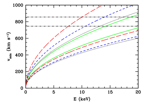
Figure 1: The minimum WIMP speed, $v_{\rm min}$, which can cause a recoil of energy $E$ for ${}^{3}{\rm He}$ (solid), C (dotted), F (short dashed) and S (long dashed) for (top and bottom curves in each case respectively) $m_{\chi}=5$ and $10\,{\rm GeV}.$ The horizontal dot-dashed lines show the maximum WIMP speeds in the lab, $v_{\chi}^{\rm max}\approx v_{\rm esc}+248{\rm km}\,{\rm s}^{-1}$, corresponding to the 90$\%$ upper and lower confidence limits on the escape speed from RAVE, $v_{\rm esc}^{\rm max}=608\,{\rm km}\,{\rm s}^{-1}$ and $v_{\rm esc}^{\rm min}=498\,{\rm km}\,{\rm s}^{-1}$.

Fig. 1 shows $v_{\rm min}$ as a function of $E$ for $m_{\chi}=5$ and $10$ GeV for ${}^{3}{\rm He}$, ${\rm C}$, ${\rm S}$ and ${\rm F}$ target nuclei. The horizontal lines show the maximum WIMP speeds in the lab, $v_{\chi}^{\rm max}=v_{\rm esc}+v_{\rm lab}^{\rm max}$, corresponding to the 90$\%$ upper and lower confidence limits on the escape speed from RAVE, $v_{\rm esc}^{\rm max}=608\,{\rm km}\,{\rm s}^{-1}$ and $v_{\rm esc}^{\rm min}=498\,{\rm km}\,{\rm s}^{-1}$. For light WIMPs, unless the target nuclei are light and the threshold energy low, the minimum speed corresponding to the threshold energy lies in the tail of the speed distribution, and in some cases beyond the cut-off due to the Galactic escape speed. The expected event rates are therefore very sensitive to the value of the escape speed and the shape of the high speed tail of the distribution.

The standard halo model, an isotropic, isothermal sphere with density profile $\rho(r)\propto r^{-2}$, is formally infinite. Hence its Maxwellian velocity distribution,

$$f({\bf v})=N\exp{\left(-\frac{3|{\bf v}|^{2}}{2\sigma^{2}}\right)}\,,\\$$ (3)

where $\sigma=\sqrt{3/2}v_{\rm c}$ and $N$ is a normalisation constant, extends to infinity too. This is usually addressed by truncating the velocity distribution by hand, either sharply or exponentially, at the escape speed.

Numerical simulations find velocity distributions with less high speed particles than the standard Maxwellian fairs ; vogelsberger ; kuhlen . Lisanti et al. lsww have presented an ansatz for the velocity distribution which reproduces this behaviour:

$$f(|{\bf v}|)\propto\left[\exp{\left(\frac{v_{\rm esc}^{2}-|{\bf v}|^{2}}{kv_{0}^{2}}\right)}-1\right]^{k}\Theta(v_{\rm esc}-|{\bf v}|)\,.$$ (4)

The parameter $k$ is related to the outer slope of the density profile, $\gamma$, ($\rho(r)\propto r^{-\gamma}$ for large $r$), by $k=\gamma-3/2$ for $\gamma>3$ kochanek .

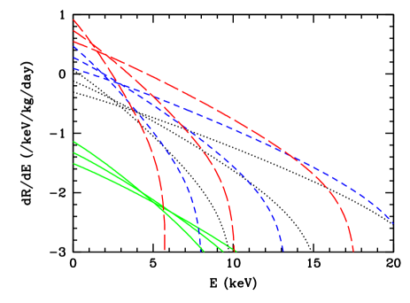
Figure 2: The differential event rates, assuming a Maxwellian speed distribution with a sharp cut-off at $v_{\rm esc}^{\rm max}=608\,{\rm km\,s}^{-1}$, a cross-section $\sigma_{\rm p}=10^{-4}\,{\rm pb}$ and a local WIMP density $\rho=0.3\,{\rm GeV}\,{\rm cm}^{-3}$, for He (solid), C (dotted), F (short dashed) and S (long dashed) for (from top to bottom at $E=0\,{\rm keV}$) $m_{\chi}=5,7.5$ and $10\,{\rm GeV}.$

We consider 2 forms for $f({\bf v})$ chosen to have high speed tails which roughly span the plausible range. Firstly, a Maxwellian distribution, eq. (3), with a sharp cut-off ($f({\bf v})=0$ for $|{\bf v}|\geq v_{\rm esc}^{\rm max}$) at the upper limit on the escape speed from RAVE, $v_{\rm esc}^{\rm max}=608\,{\rm km\,s}^{-1}$, which provides a large tail event rate. Secondly, a Lisanti et al. $f(v)$, eq. (4), with $v_{\rm esc}=v_{\rm esc}^{\rm min}=498\,{\rm km\,s}^{-1}$ to provide a small tail event rate. We fix $k=1.5$, corresponding to an outer density profile slope $\gamma=3$ and $v_{0}=v_{\rm c}=220\,{\rm km\,s}^{-1}$. In both cases we fix the local density to be $\rho=0.3\,{\rm GeV}\,{\rm cm}^{-3}$. Scaling the event rates and exposures to other densities is straight-forward.

Fig. 2 shows the differential event rates for each of the WIMP masses and targets we consider calculated using the Maxwellian distribution with a sharp cut-off at $v_{\rm esc}^{\rm max}=608\,{\rm km\,s}^{-1}$. The much smaller event rates for ${\rm He}$ are largely due to the $A^{2}$ factor in the event rate for spin-independent scattering. For heavier targets the differential event rate in the $E\rightarrow 0$ limit is substantially larger, however it decreases rapidly with increasing $E$, and the lighter the WIMP the more rapid the decrease. Furthermore for relatively small energies $v_{\rm min}$ exceeds the maximum WIMP speed in the lab frame and hence the differential event rate is zero.

Fig. 3 shows the ratio of the speed integral,

$$g(v_{\rm min})=\int_{v_{\rm min}}^{\infty}\frac{f(v)}{v}\,{\rm d}v\,,$$ (5)

for Lisanti et al.’s $f(v)$ in eq. (4) with $v_{\rm esc}^{\rm min}=498\,{\rm km\,s}^{-1}$ to that for the Maxwellian distribution with a sharp cut-off at $v_{\rm esc}^{\rm max}=608\,{\rm km\,s}^{-1}$. It also shows the velocity integral ratios for these two models if the Earth’s orbit is neglected. For $v_{\rm min}\lesssim{\cal O}(300\,{\rm km}\,{\rm s}^{-1})$ the difference in the speed integrals for the two speed distributions is relatively small, less than $10\%$. As $v_{\rm min}$ is increased, so that only the tail of the speed distribution is included in the speed integral, the difference becomes substantially larger, reaching roughly an order of magnitude for $v_{\rm min}\sim 650\,{\rm km}\,{\rm s}^{-1}$. Neglecting the Earth’s orbit has a significant ($>10\%$) effect, for $v_{\rm min}$ within $\sim 100\,{\rm km}\,{\rm s}^{-1}$ of the maximum WIMP speed in the lab frame $v_{\chi}^{\rm max}$. Therefore the Earth’s orbital speed must be included, and averaged over, for an accurate calculation of the event rate.

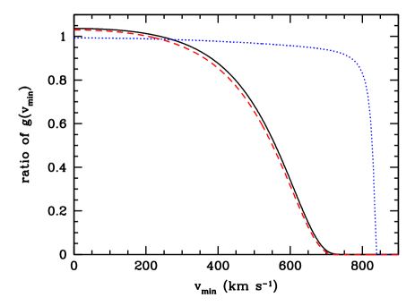
Figure 3: The speed integral, $g(v_{\rm min})$, relative to that for the Maxwellian distribution with a sharp cut-off at $v_{\rm esc}^{\rm max}=608\,{\rm km\,s}^{-1}$, including averaging over the Earth’s orbit. The solid line is for Lisanti et al.’s $f(v)$, eq. (4), with $v_{\rm esc}^{\rm min}=498\,{\rm km\,s}^{-1}$, including the Earth’s orbit. The dotted and dashed lines are for the Maxwellian and Lisanti et al. distributions respectively, neglecting the Earth’s orbit.

Simulated dark matter halos have velocity distributions which contain features at high speeds vogelsberger ; kuhlen . More specifically there are fairly broad features, which are similar at different positions within a single halo, but which vary from halo to halo, and are hence thought to be a relic of the formation history of the halo vogelsberger ; kuhlen ; ls . Ref. kuhlen also finds narrow features in some locations, corresponding to tidal streams, while Ref. purcell finds that the dark matter streams from the Sagittarius dwarf are significantly more extended than the stellar streams, and the leading dark matter stream may pass through the Solar neighbourhood. The detailed shape of the high speed tail of $f(v)$ would affect the interpretation of the CoGeNT, CRESST and DAMA data, in particular the values of the WIMP mass extracted. Since no detailed study of this has been carried out to date , we do not include the high speed features in our analysis. We defer a general investigation of the directional event rate produced by simulation velocity distributions to future work inprep .

II.4 Statistical tests

We follow the statistical procedures described in detail in Refs. pap1 ; pap3 . We use the Rayleigh-Watson statistic, which uses the mean resultant length of the recoil direction vectors. We also use the Bingham statistic which, unlike the Rayleigh-Watson statistic, can be used with axial data (where the senses of the nuclear recoils are not measured). These statistics are described in more detail in Appendices A and B.

For each WIMP mass, target nuclei and energy threshold combination we calculate the probability distribution of each statistic for WIMP induced recoils and also for the null hypothesis of isotropic recoils. We use these distributions to calculate the rejection and acceptance factors, $R$ and $A$. The rejection factor gives the confidence level with which the null hypothesis can be rejected given a particular value of the test statistic, while the acceptance factor is the probability of measuring a larger value of the test statistic if the alternative hypothesis is true. We then find the number of events required for $A=R=0.95,0.997\,30$ and $0.999\,999\,427$ i.e. to reject isotropy at this confidence level in this percentage of experiments (see Refs. pap1 ; pap3 for further discussion). The later two confidence levels correspond, for a gaussian distribution, to three and five sigma respectively. Since our aim is to examine whether directional detection experiments could detect light WIMPs we will focus on the case $A=R=0.999\,999\,427$, corresponding to the ‘five sigma’ result conventionally required for discovery.

III Results and discussion

For each of the combinations of WIMP mass, target nuclei, energy threshold and confidence level discussed in Sec. II we calculate the number of events required to reject isotropy, $N_{\rm iso}$, for vector and axial data (using the Rayleigh-Watson and Bingham statistics respectively). The number of events required for a $5\sigma$ detection with the Rayleigh-Watson statistic varies from 7 to 58. For fixed WIMP and target mass, $N_{{\rm iso}}$ decreases with increasing energy threshold, $E_{\rm th}$, (since the recoils caused by high speed WIMPs in the tail of the distribution are more anisotropic), until the minimum speed required to cause a recoil of energy $E_{\rm th}$, $v_{\rm min}(E_{\rm th})$, exceeds the maximum WIMP speed in the lab frame, $v_{\chi}^{\rm max}$. At this point the event rate is zero and no events can be detected. The same trend occurs for decreasing WIMP mass (with threshold energy and target mass fixed). For fixed threshold energy, $N_{{\rm iso}}$ decreases with increasing target mass for $m_{\chi}=5\,{\rm GeV}$, however for $m_{\chi}=7.5$ and $10\,{\rm GeV}$, $N_{{\rm iso}}$ increases as the target mass number is increased from $A=3$ to $12$ before decreasing as $A$ is increased further. This is due to the variation of $v_{\rm min}$ with target and WIMP mass shown in Fig. 1.

For the Bingham statistic, which can be used with axial data, the number of events required for a $5\sigma$ detection varies from 9 to more than 190 . Both the number of events and its increase, relative to the number required for the Rayleigh-Watson statistic, is smallest for the configurations which are only sensitive to the highly anisotropic recoils from high speed WIMPs in the tail of the speed distribution.

Figure 4: The exposure required for a $5\sigma$ rejection of isotropy as a function of energy threshold, $E_{\rm th}$, for ${}^{3}{\rm He}$ (top left), C (top right), F (bottom left) and S (bottom right) for $m_{\chi}=5,7.5$ and $10\,{\rm GeV}$ (crosses, stars and triangles respectively) for the Maxwellian $f(v)$ with a sharp cut-off at $v_{\rm esc}^{\rm max}=608\,{\rm km\,s}^{-1}$. Where a symbol is not displayed, the minimum WIMP speed corresponding to the energy threshold, $v_{\rm min}(E_{\rm th})$, for this WIMP and target mass combination exceeds the maximum WIMP speed in the lab frame, $v_{\chi}^{\rm max}$ and hence the event rate is zero.

If an experiment is only sensitive to high speed WIMPs, fewer events are required to reject isotropy, how- ever, the reduced event rate means that the exposure required to accumulate these events will be larger. We therefore use eq. (1) to calculate the exposure, ${\cal E}$, (in ${\rm kg\,day}$) required to accumulate the required number of events for each case. As illustrated in Fig. 2, for light WIMPs the differential event rate decreases rapidly with increasing energy, and therefore the event rate above the energy threshold, $R(>E_{\rm th})$, plays a crucial role in determining the exposure required.

The exposure required to reject isotropy at $5\sigma$ using the Rayleigh-Watson statistic assuming a Maxwellian $f(v)$ with a sharp cut-off at $v_{\rm esc}^{\rm max}=608\,{\rm km\,s}^{-1}$ is shown for each configuration in Fig. 4. While $N_{{\rm iso}}$ varies by less than an order of magnitude, because of the large variation in $R(>E_{\rm th})$, the exposure varies by more than five orders of magnitude. Due to the rapid decrease of $R(>E_{\rm th})$, the exposure increases sharply with increasing $E_{\rm th}$ for each WIMP and target nuclei mass combination. The factor by which the exposure increases, increases with both decreasing WIMP mass and increasing target nuclei mass (i.e. as the minimum WIMP speed to which the experiment is sensitive is increased). Eventually the minimum WIMP speed corresponding to the energy threshold, $v_{\rm min}(E_{\rm th})$, exceeds the maximum WIMP speed in the lab frame, $v_{\chi}^{\rm max}$, and the event rate is zero and WIMPs of this mass can not be detected.

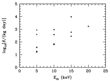
Figure 5: As Fig. 4 but for a S target only comparing the exposures required for the Lisanti et al. $f(v)$, eq. (4), with $v_{\rm esc}^{\rm min}=498\,{\rm km\,s}^{-1}$ (upper symbols) with those for the Maxwellian $f(v)$ with a sharp cut-off at $v_{\rm esc}^{\rm max}=608\,{\rm km\,s}^{-1}$ (lower symbols). For $m_{\chi}=7.5\,{\rm keV}$ and $E_{\rm th}=5\,{\rm keV}$ the exposures required for the two speed distributions are the same, and hence only one symbol is visible.

Of the halo models considered, the Maxwellian $f(v)$ with a sharp cut-off at $v_{\rm esc}^{\rm max}=608\,{\rm km\,s}^{-1}$ has the largest tail event rate, and hence the smallest exposures. In Fig. 5 we show the exposures for a ${\rm S}$ target for the Lisanti et al. $f(v)$, eq. (4), with $v_{\rm esc}^{\rm min}=498\,{\rm km\,s}^{-1}$ as well. When $v_{\rm min}(E_{\rm th})$ is much smaller than $v_{\chi}^{\rm max}$ the exposure required is fairly modest, ${\cal E}\sim 10-100\,{\rm kg}\,{\rm day}$ and the event rates, and hence exposures, for the two speed distributions are very similar. However as $v_{\rm min}(E_{\rm th})$ approaches $v_{\chi}^{\rm max}$ the exposures required become large and the differences between the two speed distributions become significant. For instance for $E_{\rm th}=20\,{\rm keV}$, WIMPs with $m_{\chi}=10\,{\rm GeV}$ and a Maxwellian distribution with $v_{\rm esc}^{\rm max}=608\,{\rm km\,s}^{-1}$ anisotropy could be detected with an exposure of $1700\,{\rm kg}\,{\rm day}$, however if the WIMPs have the Lisanti et al. $f(v)$ with $v_{\rm esc}^{\rm min}=498\,{\rm km\,s}^{-1}$ the event rate is zero and they can not be detected. The trends for the other target nuclei are similar.

In Fig. 6 we compare the exposures required to reject isotropy with axial data using the Bingham statistic with those for vectorial data using the Rayleigh-Watson statistic, for a ${\rm S}$ target and a Maxwellian $f(v)$ with a sharp cut-off at $v_{\rm esc}^{\rm max}=608\,{\rm km\,s}^{-1}$. Since $R(>E_{\rm th})$ for each configuration doesn’t change, the variations in the exposure are driven entirely by the variations in $N_{\rm iso}$ discussed above. Therefore the increase in the exposure, relative to that required for the Rayleigh-Watson statistic, is smallest for the cases which are only sensitive to the highly anisotropic recoils from high speed WIMPs in the tail of the speed distribution. However in these cases the exposure is large even for the Rayleigh-Watson statistic, due to the small values of $R(>E_{\rm th})$.

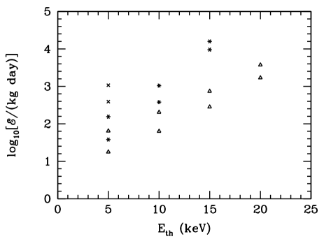
Figure 6: As Fig. 5 but comparing the exposures required using the Bingham statistic (upper symbols) with those required using the Rayleigh statistic (lower symbols), in both cases for a S target using a Maxwellian $f(v)$ with a sharp cut-off at $v_{\rm esc}^{\rm max}=608\,{\rm km\,s}^{-1}$. For $m_{\chi}=10\,{\rm GeV}$ and $E_{\rm th}=5\,{\rm keV}$ we have only been able to place a lower bound on the number of events, and hence exposure, required with the Bingham statistic.

We have focused on the number of events and exposure required for a ‘$5\sigma$’ discovery of light WIMPs with a directional detector. Significant experimental support for light WIMPs would be obtained even with a lower significance signal. For $95\%$ and $99.713\%$ confidence levels (the later corresponding to $3\sigma$) the number of events, and hence the exposure, required with the Rayleigh-Watson statistic is smaller by a factor of between $0.40-0.91$ and $0.69-0.95$ respectively. The factor by which the number of events must be increased to increase the significance of the rejection of isotropy is smallest when the experiment is only sensitive to the most anisotropic events coming from the tail of the speed distribution. However in these cases the exposure required even for a low significance detection is large.

The final question is ‘How achievable are these exposures and energy thresholds by current and near-future detectors’? A typical current detector consisting of a $1\,{\rm m}^{3}$ TPC filled to 75 Torr with ${\rm CF}_{4}$ or ${\rm CS}_{2}$ could, in roughly a year, achieve an exposure of order $10^{3}\,{\rm kg\,day}$ cygnus . A $10^{3}\,{\rm kg\,day}$ exposure with ${\rm CF}_{4}$ or ${\rm CS}_{2}$ would (provided that recoils are measured in 3d with good, $\lesssim 10^{\circ}$, angular resolution) be capable of detecting $m_{\chi}=10\,{\rm keV}$ WIMPs with an energy threshold of $20\,{\rm keV}$ or lower. Lighter WIMPs would require a lower energy threshold, potentially as low as $5\,{\rm keV}$ for $m_{\chi}=5\,{\rm GeV}$. With a ${}^{3}{\rm He}$ target a low, $\sim 5\,{\rm keV}$, energy threshold would be required, even for $m_{\chi}=10\,{\rm GeV}$. Measuring the directions of low energy nuclear recoils is a major experimental challenge, and these energy threshold are lower than those which have been used in the analysis of data from current, prototype, detectors cygnus . One of the focuses of the R&D for future generation experiments is to reduce the energy threshold (see e.g. cygtalks ). The MIMAC experiment has, using micromegas readout, detected 5 keV F recoils mimaclow , while DRIFT-II is sensitive to nuclear recoils down to sub $5$ keV energies driftlow . Simulations of the MIMAC detector indicate that the directional energy threshold will lie below $20$ keV billardtrack

IV Summary

The event rate excess and annual modulations observed by various direct detection experiments may be due to light, $5-10\,{\rm GeV}$ WIMPs. We have investigated whether near future directional detection experiments will be able to test this possibility, by detecting the anisotropy of the nuclear recoils. We find, using the Rayleigh-Watson statistic, that an ideal directional detector (capable of measuring the directions of the recoils, including their senses, in 3d with good angular resolution) would require between 7 and 58 events to detect the anisotropy at $5\sigma$. The number of events required depends on the target nuclei mass, energy threshold, WIMP mass, and crucially the details of the high speed tail of the WIMP speed distribution. It is smallest for cases where the experiment is only sensitive to the highly anisotropic recoils from high speed WIMPs in the tail of the speed distribution. If the detector is not capable of measuring the senses of the recoils we find, using the Bingham statistic, that the number of events required ranges between 9 and more than 190. The increase in the number of events required with axial data is smallest for the cases which are only sensitive to high speed WIMPs due to the higher degree of anisotropy in the nuclear recoil distributions.

In terms of the detection potential the key quantity is the exposure necessary to detect the required number of events, which is inversely proportional to the event rate above threshold. For the configurations we have considered (${}^{3}{\rm He}$, C, F and S targets, $5-10\,{\rm GeV}$ WIMPs and energy threshold between $5$ and $20\,{\rm keV}$) the event rate above threshold varies by more than five orders of magnitude, and in some cases the minimum speed required to cause a recoil above threshold exceeds the maximum WIMP speed in the lab and the event rate is zero. For the cases which are only sensitive to high speed WIMPs, where the number of events required was smallest, the event rate above threshold is small and hence very large exposures would be required. The shape of the high speed tail of the WIMP distribution is not well known and this leads to large uncertainties in the event rate expected in experiments which are only sensitive to the high speed tail, c.f. Refs. lsww ; fpsv ; mmm ; mccabe . We also emphasize that including, and averaging over, the Earth’s orbit is essential for an accurate calculation of the event rate in these cases.

We find that a future ${\rm CF}_{4}$ or ${\rm CS}_{2}$ detector with an energy threshold of $20\,{\rm keV}$ or lower, which can measure recoil directions and senses in 3d with good angular resolution, would be capable of detecting WIMPs with $(m_{\chi},\sigma_{p})=(10\,{\rm GeV},10^{-4}\,{\rm pb})$ with an exposure of $10^{3}\,{\rm kg\,day}$. Detecting lighter WIMPs would require a lower energy threshold. With a ${}^{3}{\rm He}$ target a low, $\sim 5\,{\rm keV}$, energy threshold would be required, even for WIMP masses at the upper end of the mass range considered. In summary, we conclude that directional detection experiments may be able to detect light WIMPs, but this depends quite sensitively on both the experimental configuration (target nuclei mass and energy threshold) and the unknown WIMP mass and velocity distribution. The directional energy thresholds required to detect light WIMPs are below those used in analyses of data from current directional detectors, however it has been demonstrated that directional detectors can detect mimaclow ; driftlow and measure the directions billardtrack of low energy nuclear recoils and R&D is underway to realise lower energy thresholds cygtalks .

We also note that directional experiments, with heavy targets, could also test inelastic dark matter as the explanation of the direct detection anomalies inelastic .

Appendix A Rayleigh Watson statistic

The (modified) Rayleigh-Watson statistic, ${\cal W}^{\star}$ is the simplest coordinate independent statistic for detecting anisotropy in vectorial data. It is related to the Rayleigh statistic, ${\cal R}$, which for a sample of $N$ unit vectors $\vec{x}_{i}$ is given by

$${\cal R}=\left|\sum^{N}_{i=1}\vec{x}_{i}\right|\,.$$ (6)

i.e. the modulus of the sum of vectors. For an isotropic data set ${\cal R}$ should be zero, modulo statistical fluctuations. For anisotropic data the value of ${\cal R}$ becomes larger as the degree of anisotropy increases.

The modified Rayleigh-Watson statistic, ${\cal W}^{\star}$, defined as watson1 ; watsonbook ; mardia:jupp

$${\cal W}^{\star}=\left(1-\frac{1}{2N}\right){\cal W}+\frac{1}{10N}{\cal W}^{2}\,,$$ (7)

where ${\cal W}$ is the (unmodified) Rayleigh-Watson statistic

$${\cal W}=\frac{3}{N}{\cal R}^{2}\,.$$ (8)

The modified statistic ${\cal W}^{\star}$ has the advantage of approaching its large $N$ asymptotic distribution for smaller $N$ than the unmodified statistic. For isotropically distributed vectors, ${\cal W}^{\star}$ is asymptotically distributed as $\chi^{2}_{3}$ watson1 ; watsonbook . The difference between $\chi^{2}_{3}$ and the true distribution of ${\cal W}^{\star}$ for isotropic vectors in the large ${\cal W}^{\star}$ tail of the distribution is less than $2\%$ for $N>30$ pap1 . For smaller $N$ the $\chi^{2}_{3}$ distribution significantly underestimates the true probability distribution and therefore, as in Ref. pap1 we calculate the probability distribution from the exact probability distribution of ${\cal R}$, as described in Ref. stephens:rayleigh .

Appendix B Bingham statistic

The Rayleigh-Watson statistic can not be used with axial data, as it is not sensitive to distributions which are symmetric with respect to the centre of the sphere. For axial data the Bingham statistic ${\cal B}^{\star}$ which is based on the scatter matrix of the data, ${\bf T}$, can be used. This matrix is defined as watson2 ; watsonbook ; mardia:jupp

$${\bf T}=\frac{1}{N}\sum^{N}_{i=1}\left(\begin{array}[]{ccc}x_{i}x_{i}&x_{i}y_{i}&x_{i}z_{i}\\ y_{i}x_{i}&y_{i}y_{i}&y_{i}z_{i}\\ z_{i}x_{i}&z_{i}y_{i}&z_{i}z_{i}\end{array}\right)\,,$$ (9)

where $(x_{i},y_{i},z_{i})$ are the components of the $i$-th vector or axis. This matrix is real and symmetric with unit trace, so that that the sum of its eigenvalues $e_{k}$ ($k=1,2,3$) is unity, and for an isotropic distribution all three eigenvalues should, modulo statistical fluctuations, be equal to $1/3$. The Bingham statistic, ${\cal B}$,

$${\cal B}=\frac{15N}{2}\sum^{3}_{k=1}\left(e_{k}-\frac{1}{3}\right)^{2}\,,$$ (10)

measures the deviation of the eigenvalues $e_{k}$ from the value of 1/3 expected for an isotropic distribution. For isotropically distributed vectors/axes ${\cal B}$ is asymptotically distributed as $\chi^{2}_{5}$. Since ${\bf T}$ is symmetric under a sign change of $\vec{x}$, the Bingham statistic can be used for axial data as well as vectors.

References

- (1) M. W. Goodman and E. Witten, Phys. Rev. D 31, 3059 (1985).
- (2) B. Bertone, D. G. Cerdeno, M. Fornasa, R. Ruiz de Austri, C. Strege and R. Trotta, JCAP01(2012)015, arXiv:1107.1715.
- (3) R. Bernabei et al., Eur. Phys. C 56, 39 (2010), arXiv:1002.1028.
- (4) A. Bottino, F. Donato, N. Fornengo and S. Scopel, Phys. Rev. D 69 (2004) 037302 [hep-ph/0307303].
- (5) G. B. Gelmini and P. Gondolo, Phys. Rev. D 74 123520 (2005), arXiv:0504010.
- (6) C. E. Aalseth et al., Phys. Rev. Lett. 106, 131301 (2011), arXiv:1002.4703.
- (7) C. E. Aalseth et al., Phys. Rev. Lett. 107, 141301 (2011), arXiv:1106.0650.
- (8) A. K. Drukier, K. Freese and D. N. Spergel, Phys. Rev. D 33, 3495 (1986).
- (9) G. Angloher et al., Eur. Phys. J. C 72, 1971 (2012), arXiv:1109.0702.
- (10) D. S. Akerib et al., Phys. Rev. D 82, 122004 (2010), arXiv:1010.4290.
- (11) J. Angle et al., Phys. Rev. Lett. 107 051301 (2011), arXiv:1104.3088.
- (12) E. Aprile et al., Phys. Rev. Lett. 107 131302 (2011), arXiv:1104.2549; arXiv:1207.5988.
- (13) A. Brown, S. Henry, H. Kraus and C. McCabe, Phys. Rev. D 85, 021301 (2012), arXiv:1109.2589.
- (14) J. Kopp, T. Schwetz and J. Zupan, JCAP03(2012)001, arXiv:1110.2721.
- (15) C. Kelso, D. Hooper and M. R. Buckley, Phys. Rev. D 85 043515 (2012), arXiv:1110.5338.
- (16) M. T. Frandsen, F. Kahlhoefer, C. McCabe, S. Sarkar and K. Schmidt-Hoberg, JCAP01(2012)024, arXiv:1111.0292.
- (17) D. Hooper and C. Kelso, Phys. Rev. D 84 083001 (2011), arXiv:1106.1066.
- (18) T. Schwetz and J. Zupan, JCAP08(2011)009, arXiv:1106.6241; C. McCabe, Phys. Rev. D 84 043525 (2011), arXiv:1107.0741; P. J. Fox, J. Kopp, M. Lisanti and N. Weiner, Phys. Rev. D 85 036008 (2012), arXiv:1107.0717.
- (19) J. Cherwinka et al., Astropart. Phys. 35, 749 (2012), arXiv:1106.1156.
- (20) D. N. Spergel, Phys. Rev. D 67, 1353 (1988).
- (21) C. J. Copi, J. Heo and L. M. Krauss, Phys. Lett. B 461, 43 (1999), astro-ph/990449; C. J. Copi and L. M. Krauss, Phys. Rev. D 63, 043507 (2001), astro-ph/0009467.
- (22) B. Morgan, A. M. Green and N. J. C. Spooner, Phys. Rev. D 71 103507 (2005), astro-ph/0408047.
- (23) N. Bozorgnia, G. B. Gelmini and P. Gondolo, JCAP06(2012)037, arXiv:1111.6361.
- (24) J. Billard, F. Mayet, J. F. Macias-Perez and D. Santos, Phys. Lett. B 691, 156 (2010), arXiv:0911.4086.
- (25) A. M. Green and B. Morgan, Phys. Rev. D 81, 061301 (2010), arXiv:1002.2717.
- (26) B. Morgan and A. M. Green, Phys. Rev. D 72, 123501 (2005), astro-ph/0508134.
- (27) A. M. Green and B. Morgan, JCAP08(2007)022, astro-ph/0609115.
- (28) G. Sciolla and C. J. Martoff, New J. Phys. 11 105018 (2009), arXiv:0905.3675.
- (29) S. Ahlen et al., Int. J. Mod. Phys. A 25 1-51 (2010), arXiv:0911.0323.
- (30) G. Sciolla et al., J. Phys. Conf. Ser. 179 012009 (2009), arXiv:0903.3895; S. Ahlen et al., Phys. Lett. B 695, 124 (2011), arXiv:1006.2928; J. B. R. Battat et al., arXiv:1109.3270.
- (31) D. P. Snowden-Ifft, C. J. Martoff, and J. M. Burwell, Phys. Rev. D 61, 1 (2000), astro-ph/9904064; G. J. Alner et al., Nucl. Inst. and Meth. A. 535, 644 (2004); E. Daw et al., arXiv:1110.0222.
- (32) D. Santos et al., J. Phys. Conf. Ser. 309 (2011) 012014, arXiv:1102.3265.
- (33) T. Tanimori et al., Phys. Lett. B 578, 241 (2004) astro-ph/0310638; K. Miuchi et al., Phys. Lett. B 686, 11 (2010), arXiv:1002.1794; K. Miuchi et al., 1109.3099.
- (34) J. Billard, F. Mayet and D. Santos, JCAP04(2012) 006, arXiv: 1202.3372.
- (35) C. J. Copi, L. M. Krauss, D. Simmons-Duffin and S. R. Stroiney, Phys. Rev. D 75, 023614 (2007), astro-ph/0508649.
- (36) J. Billard, F. Mayet and D. Santos, Phys. Rev. D 85, 035006 (2012), arXiv:1110.6079.
- (37) M. S. Alenazi and P. Gondolo, Phys. Rev. D 77 043532 (2008), arXiv:0712.0053.
- (38) A. M. Green and B. Morgan, Phys. Rev. D 77 027303 (2008) (4 pages), arXiv:0711.2234.
- (39) M. C. Smith et al., Mon. Not. Roy. Astron. Soc. 379, 755 (2007), astro-ph/0611671.
- (40) P. J. McMillan and J. J. Binney, Mon. Not. Roy. Astron. Soc. 402 934 (2010), arXiv:0907.4685.
- (41) M. Brhlik and L. Roszkowski, Phys. Lett. B 464, 303 (1999), hep-ph/9903468.
- (42) A. M. Green, JCAP10(2010)034, arXiv:1009.0916.
- (43) J. March-Russell, C. McCabe and M. McCullough, JHEP05(2009)071, arXiv:0812.1931.
- (44) C. McCabe, Phys. Rev. D 82 023530 (2010), arXiv:1005.0579.
- (45) C. Savage, K. Freese, P.Gondolo and D. Spolyar, JCAP09(2009)036, arXiv:0901.2713.
- (46) M. Kamionkowski and A. Kinkhabwala, Phys. Rev. 57 3256 (1998), hep-ph/9710337.
- (47) M. Lisanti, L. E. Stigari, J. G. Wacker and R. H. Wechsler, Phys. Rev. D 83 023519, arXiv:1010.4300.
- (48) M. Farina, D. Pappadopulo, A. Strumia and T. Volansky, JCAP11(2011)010, arXiv:1107.0715.
- (49) P. S. Behrozzi, A. Loeb and R. H. Wechsler, arXiv:1208.0334.
- (50) R. Schoenrich, J. Binney and W. Dehnen, Mon. Not. Roy. Astron. Soc. 403, 1829 (2010), arXiv:0912.3693.
- (51) M. Fairbairn and T. Schwetz, JCAP01(2009)037, arXiv:0808.0704.
- (52) M. Vogelsberger et al., Mon. Not. Roy. Astron. Soc. 395, 797 (2009), arXiv:0812.0362.
- (53) M. Kuhlen et al., JCAP02(2010)030, arXiv:0912.2358.
- (54) C. S. Kochanek, Astrophys. J 457, 228 (1996).
- (55) M. Lisanti and D. N. Spergel, arXiv:1105.4166; M. Kuhlen, M. Lisanti and D. N. Spergel, arXiv:1202.0007.
- (56) C. W. Purcell, A. R. Zentner and M-Y Wang, arXiv:1203.6617.
- (57) A. Natarajan, C. Savage and K. Freese., Phys. Rev. D 84 103005 (2011), arXiv:1109.0014.
- (58) A. M. Green and B. Morgan, in preparation.
- (59) Various talks at ‘CYGNUS 2011: 3rd Workshop on directional detection of Dark Matter’, http://lpsc.in2p3.fr/Indico/conferenceTimeTable.py?confId=466#20110607
- (60) D. Santos et al. arXiv:1111.1566.
- (61) S. Burgos et al., JINST 4 P04014 (2009), arXiv:0903.0326.
- (62) D. P. Finkbeiner, T. Lin and N. Weiner, Phys. Rev. D 80, 115008, arXiv:0906.002; M. Lisanti and J. G. Wacker, Phys. Rev. D 81 096005 (2010), arXiv:0911.1997.
- (63) G. S. Watson, Geophys. Suppl. Mon. Not. Roy. Astron. Soc. 7, 160 (1956).
- (64) G. S. Watson, Statistics on Spheres, Wiley, New York (1983).
- (65) K. V. Mardia and P. Jupp, Directional Statistics, Wiley, Chichester (2002).
- (66) M. A. Stephens, J. Amer. Statist. Assoc. 59, 160 (1964).
- (67) G. S. Watson, J. Geol. 74, 786 (1966).
- (68) C. Bingham, Ann. Stat. 2, 1201 (1974).