Phases of supersymmetric $O(N)$ theories

Abstract

We perform a global renormalization group study of $O(N)$ symmetric Wess-Zumino theories and their phases in three euclidean dimensions. At infinite $N$ the theory is solved exactly. The phases and phase transitions are worked out for finite and infinite short-distance cutoffs. A distinctive new feature arises at strong coupling, where the effective superfield potential becomes multi-valued, signalled by divergences in the fermion-boson interaction. Our findings resolve the long-standing puzzle about the occurrence of degenerate $O(N)$ symmetric phases. At finite $N$, we find a strongly-coupled fixed point in the local potential approximation and explain its impact on the phase transition. We also examine the possibility for a supersymmetric Bardeen-Moshe-Bander phenomenon, and relate our findings with the spontaneous breaking of supersymmetry in other models.

I Introduction

Supersymmetry, the symmetry which links bosonic with fermionic degrees of freedom, is an intriguing concept with many applications in quantum field theory and statistical physics. It plays a prominent role for open challenges in the Standard Model of Particle Physics such as the hierarchy problem, and continues to inspire the construction of models for new physics. In statistical physics, supersymmetry also appears as a technical symmetry in the exploitation of systems which otherwise are too difficult to handle. It is thus of great interest to further the understanding of interacting supersymmetric theories, and to clarify the impact of supersymmetry on the phase structure and the critical behavior at lowest and highest energies.

This work is devoted to the supersymmetric extension of $O(N)$ symmetric scalar theories in three euclidean dimensions, continuing a line of research initiated in Litim:2011bf . Without supersymmetry, the bosonic theory with a microscopic $(\phi^{2})^{3}$ potential is described by three renormalized parameters permitting first-order phase transitions at strong coupling as well as second order phase transitions with Ising-type critical behavior ZinnJustin . In the limit of infinitely many scalars, the analytically solvable spherical model also admits an ultraviolet fixed point with broken scale invariance, the Bardeen-Moshe-Bander (BMB) phenomenon, allowing for a non-trivial continuum limit Bardeen:1983rv ; David:1984we ; David:1985zz . With supersymmetry, additional fermionic degrees of freedom are present and their fluctuations modify the quantum effective theory. The $O(N)$ symmetric Wess-Zumino model with a microscopic $(\Phi^{2})^{2}$ superpotential is determined by only two renormalized parameters and critical and tricritical theories are the same. Its phase structure has attracted some attention in the past Bardeen:1984dx ; Moshe:2003xn ; Dawson:2005uw ; Suzuki:1985uk ; Suzuki:1985pw ; Gudmundsdottir:1984yk ; Feinberg:2005nx ; Matsubara:1987iz . In the limit of infinitely many superfields, four different phases have been observed Bardeen:1984dx ; Moshe:2003xn , including peculiar degenerate $O(N)$ symmetric phases with several mass scales. Similar to the scalar case, a supersymmetric version of the BMB fixed point has equally been found at a critical coupling where the bosons and fermions become massive while a Goldstone-boson (dilaton) and a Goldstone-fermion (dilatino) are dynamically generated. The supersymmetric $O(N)$ model has also been discussed in the $1/N$ expansion Gudmundsdottir:1984yk , where the authors found a non-trivial UV fixed-point and a stable dilaton phase. At next-to-leading order the dilaton acquires a mass of order $1/N$ showing that a phase with spontaneously broken scale invariance only exists in the limit of infinitely many superfields Matsubara:1987iz .

A method of choice in the study of phases and phase transitions is Wilson’s renormalisation group (RG) Wetterich:1992yh . It is based on a path-integral representation of the theory, where the continuous integrating-out of momentum modes permits a smooth and controlled interpolation between the microscopic and the full quantum effective theory Berges:2000ew . Physically-motivated approximations schemes together with analytic versions of the RG Litim:2000ci ; Litim:2001fd ; Litim:2001up allow for a global analysis and a classification of phase transitions and critical exponents even at strong coupling. The method has been successfully applied to phase transitions in Ising-type universality classes Tetradis:1992xd ; Tetradis:1995br ; Berges:2000ew ; Bagnuls:2000ae including high-precision computations of its critical exponents with increasing levels of sophistication Litim:2002cf ; Litim:2003kf ; Canet:2003qd ; Bervillier:2007rc ; Benitez:2009xg ; Litim:2010tt . The extension of the functional RG towards supersymmetric theories Vian:1998kv ; Bonini:1998ec ; Synatschke:2008pv ; Gies:2009az ; Synatschke:2009nm ; Synatschke:2010jn ; Synatschke:2010ub ; Synatschke:2009da ; Falkenberg:1998bg ; Rosten:2008ih ; Sonoda:2009df ; Sonoda:2008dz ; Litim:2011bf therefore bears the promise for deeper insights into the phases and the critical behavior of supersymmetric $O(N)$ theories.

This paper is organized as follows: We recall the main features of supersymmetric $O(N)$ models including a supersymmetric version of Wilson’s RG (Sec. II), followed by a discussion of its exact analytical solution in the large-$N$ limit (Sec. III). We then give a detailed account of the phase diagram and phase transitions in the renormalized theory, and examine the appearance of a multi-valued effective potential, also in comparison with earlier findings (Sec. IV). We repeat this exercise with a finite short-distance cutoff including a thermodynamical derivation of scaling exponents (Sec. V), and examine the supersymmetric BMB phenomenon (Sec. VI). At finite $N$, we derive an exact fixed point to leading order in a gradient expansion and evaluate its impact on the phase transition, and on the fate of the BMB mechanism (Sec. VII). We close with a brief summary and some conclusions (Sec. VIII).

II Supersymmetric RG flow

In this section we sketch the features of supersymmetric $O(N)$ models and recall the supersymmetric renormalization group flow in the local potential approximation. For a detailed discussion and derivation see Litim:2011bf .

II.1 Action

The three-dimensional supersymmetric $O(N)$ models are built from $N$ real superfields

$$\Phi_{i}(x,\theta)=\phi_{i}(x)+\bar{\theta}\psi_{i}(x)+\frac{1}{2}\bar{\theta}\theta F_{i}(x)$$ (1)

containing scalar fields $\phi_{i}$, Majorana fermions $\psi_{i}$ and auxiliary fields $F_{i}$ as components and a two-component anticommuting Majorana spinor $\theta$. The invariant action

$$S=\int d^{3}x\,\left.\left(-\frac{1}{2}\Phi\,\bar{\mathcal{D}}\,\mathcal{D}\,\Phi+2W(R)\right)\right|_{\bar{\theta}\theta}\,,$$ (2)

wherein we suppress the internal summation index $i$, contains the $O(N)$-invariant composite superfield

$$R=\frac{1}{2}\Phi^{2}=\bar{\rho}+(\bar{\theta}\psi)\phi+\frac{1}{2}\,\bar{\theta}\theta\left(\phi F-\frac{1}{2}\bar{\psi}\psi\right)\,,$$ (3)

where $\bar{\rho}\equiv\phi^{2}/2$. The supercovariant derivatives

$$\mathcal{D}=\frac{\partial}{\partial{\bar{\theta}}}+i\not{\partial}\theta\quad\mbox{and}\quad\mathcal{\bar{D}}=-\frac{\partial}{\partial\theta}-i\bar{\theta}\not{\partial}$$ (4)

obey $\{\mathcal{D}_{k},\bar{\mathcal{D}}_{l}\}=-2i(\gamma^{\mu})_{kl}\partial_{\mu}$. An expansion in component fields yields the off-shell Lagrangian density

$$\mathcal{L}_{\rm off} = \mbox{\small{$\frac{1}{2}$}}\left(-\phi\Box\phi-i\bar{\psi}\not{\partial}\psi+F^{2}\right)+W^{\prime}(\bar{\rho})\,\phi F$$ (5)

$$- \mbox{\small{$\frac{1}{2}$}}W^{\prime}(\bar{\rho})\,\bar{\psi}\psi-\mbox{\small{$\frac{1}{2}$}}W^{\prime\prime}(\bar{\rho})\,(\bar{\psi}\phi)\,(\psi\phi)\,.$$

By eliminating the auxiliary fields $F$ through their algebraic equation of motion, $F=-W^{\prime}(\bar{\rho})\,\phi$, we obtain the on-shell density. The field-dependent fermion mass $m_{\psi}$, the bosonic potential $V$, and the field-dependent Yukawa-type coupling $\lambda_{Y}$ all follow from the superpotential $W$ as

$$m_{\psi} = W^{\prime}(\bar{\rho})$$

$$V = \bar{\rho}\,\left[W^{\prime}(\bar{\rho})\right]^{2}$$ (6)

$$\lambda_{Y} = \mbox{\small{$\frac{1}{2}$}}W^{\prime\prime}(\bar{\rho})\,.$$

All salient features of the classical theory are encoded in the functions (6). For a polynomial superpotential the scalar field potential always has a minimum at $V(0)=0$ implying that global supersymmetry is unbroken.

II.2 Renormalization group

Including the effects of quantum and thermal fluctuations implies that the classical action (2) is modified and replaced by a “coarse-grained” or “flowing” effective action $\Gamma_{k}$. In the next-to-leading order in the super-derivative expansion

$$\Gamma_{k}[\Phi]= \int\!d^{3}x\,\left.\left(-\frac{1}{2}\Phi\,Z_{k}\,\bar{\mathcal{D}}\mathcal{D}\,\Phi+2\,W_{k}\right)\right|_{\bar{\theta}\theta}$$ (7)

interpolates between the classical action at the high-energy cutoff-scale $k=\Lambda$ and the full effective action at $k=0$. The fluctuations above $k$ modify both the superpotential, which has turned into a scale-dependent superpotential $W_{k}$, and the kinetic terms, which may acquire a non-trivial field- and momentum-dependent wave function renormalization factor $Z_{k}(\frac{1}{2}\Phi^{2},\bar{\mathcal{D}}\mathcal{D})$.

The RG momentum scale $k$ is introduced on the level of the path integral by adding suitable momentum cutoffs $R_{k}(q^{2})$ to the inverse propagators of the fields. The cutoffs regularizes the path integral in the infrared and gives rise to a finite flow of the scale dependent effective action. Optimized choices for $R_{k}$ are available to ensure the stability of the resulting RG equations Litim:2000ci ; Litim:2001fd ; Litim:2001up . The scale dependence of the effective action (7) is described by a functional differential equation Wetterich:1992yh

$${\partial_{t}}\Gamma_{k}=\frac{1}{2}{\rm STr}\left(\Gamma^{(2)}_{k}+R_{k}\right)^{-1}\partial_{t}R_{k}\,,$$ (8)

which emerges as an exact identity from a path integral representation. Here, $t=\ln k/\Lambda$ denotes the dimensionless RG “time” parameter, $\Gamma^{(2)}_{k}$ the second functional derivative of $\Gamma_{k}$ with respect to the fields, and the supertrace denotes a momentum integration and a sum over all fields, including appropriate minus signs for fermions.

II.3 Derivative expansion

Finally we detail our equations to leading order in a super-derivative expansion, the so-called local potential approximation (LPA). It amounts to setting the wave function factor $Z_{k}=1$ throughout, which is a good approximation in the large-$N$ limit where RG corrections to the wave function renormalization of the relevant degrees of freedom, the Goldstone modes, are suppressed as $1/N$. In scalar $O(N)$ theories, the LPA gives already very good results for scaling at the Wilson-Fisher fixed point Litim:2002cf . Here, the LPA does retain the full field- and scale-dependence of the superpotential $W_{k}$.

In this work, we introduce the momentum cutoff as a supersymmetric invariant $F$-term of the superfield, by adding $\Delta S_{k}=\mbox{\small{$\frac{1}{2}$}}\int d^{3}x\,\Phi R_{k}\Phi|_{\bar{\theta}\theta}$ to the action under the path integral, with

$$\Phi\,R_{k}(\bar{\mathcal{D}}\mathcal{D})\,\Phi=-\mbox{\small{$\frac{1}{2}$}}\Phi\,r_{k}(-\Box)\bar{\mathcal{D}}\mathcal{D}\,\Phi\,.$$ (9)

The dimensionless function $r_{k}(p^{2})$ describes the shape of the momentum cutoff. The momentum trace is performed analytically for specific optimized choices for $r_{k}$ Litim:2000ci ; Litim:2001fd ; Litim:2001up . Following Litim:2001up ; Synatschke:2010ub , we adopt

$$r_{k}(p^{2})=\left(\frac{k}{|p|}-1\right)\theta(k^{2}-p^{2})\,.$$ (10)

The flow in LPA for the superpotential is obtained by projecting (8) onto the term linear in the auxiliary field $F$, and this yields

$$\begin{split}\frac{N}{k^{2}}\partial_{t}W=-\left(N\!-\!1\right)I\left(\frac{W^{\prime}}{k}\right)-I\left(\frac{W^{\prime}\!+\!2\bar{\rho}\,W^{\prime\prime}}{k}\right),\end{split}$$ (11)

where $I(x)={x}/(1+x^{2})$. It is understood that $W$ and its derivatives are functions of the RG scale $k$ and the fields, and we will omit the index $k$. The first term on the RHS is the contribution of the $N-1$ Goldstone modes and the last term is the contribution of the radial mode. Note that the RHS of the flow vanishes for $W^{\prime}\equiv 0$, and for $1/|W^{\prime}|\to 0$, corresponding to the classical limit where the couplings and the potential (6) are independent of the RG scale.

To achieve the simple form (11) we have rescaled the fields and the superpotential as

$$\bar{\rho}\to\frac{N}{8\pi^{2}}\bar{\rho}\,,\quad W\to\frac{N}{8\pi^{2}}\,W\,.$$ (12)

Note that $W^{\prime}$ is invariant under the rescaling which absorbs the redundant overall factor $1/(8\pi^{2})$, originating from the momentum integration, into the field and the superpotential. The additional rescaling with $N$ also removes the leading $N$-dependence from the RG equation (11). In these conventions, and with given initial condition $W_{k=\Lambda}(\bar{\rho})$ the RG flow determines the superpotential in the infrared limit $k\rightarrow 0$.

To study the critical behavior we introduce a dimensionless field variable $\rho$, a dimensionless superpotential $w$ and a dimensionless scalar potential $v$ as

$$\rho = \frac{\bar{\rho}}{k},\ \ w(\rho)=\frac{W(\bar{\rho})}{k^{2}},\ \ v(\rho)=\frac{\bar{\rho}}{k}\!\left(\frac{W^{\prime}(\bar{\rho})}{k}\right)^{2}\!\!.$$ (13)

In terms of (13) the flow equation (11) reads

$$\partial_{t}w+2w-\rho w^{\prime}=-\big{(}1-\frac{1}{N}\big{)}I(w^{\prime})-\frac{1}{N}I(w^{\prime}+2\rho w^{\prime\prime})\,.$$ (14)

For completeness we add the flow equation for $w^{\prime}\equiv u$,

$$\partial_{t}u+u-\rho u^{\prime} = -\big{(}1-\frac{1}{N}\big{)}u^{\prime}\,I^{\prime}(u)$$ (15)

$$-\frac{1}{N}\left(3u^{\prime}+2\rho u^{\prime\prime}\right)I^{\prime}(u+2\rho u^{\prime})\,,\quad$$

and similarly for higher derivatives of the superpotential.

III Effective potential

In this section, we discuss the explicit and exact solution for the effective potential in the limit $1/N\to 0$, and derive the main equations which govern the symmetry breaking in this model.

III.1 RG flow and boundary condition

In the large-$N$ limit, the flow equation (15) for $u\equiv w^{\prime}$ simplifies considerably and is given by

$$\partial_{t}u+u-\rho\,u^{\prime}=-\frac{1-u^{2}}{(1+u^{2})^{2}}\,u^{\prime}\,.$$ (16)

The terms on the LHS encode the canonical scaling of the superpotential and the fields and the RHS encode the effects due to fluctuations. The integration of (16) with respect to the logarithmic RG scale $t=\ln k/\Lambda$ gives

$$\frac{\rho-1}{u}-F(u)=G(ue^{t})$$ (17)

with

$$F(u)=\frac{u}{1+u^{2}}+2\arctan(u)\,.$$ (18)

The function $G(x)$ is determined by the initial conditions for $u(\rho)$ imposed at some reference scale $k=\Lambda$. We use throughout the boundary condition

$$k=\Lambda:\quad\left\{\begin{array}[]{ll}\displaystyle u(\rho)&=\tau\,(\rho-\kappa)\\[4.30554pt] W^{\prime}(\bar{\rho})&=\tau\,(\bar{\rho}-\kappa\,\Lambda)\,,\end{array}\right.$$ (19)

where $\tau$ denotes the quartic superfield coupling at the cutoff. We recall that it is an exactly marginal coupling, i.e. that $\partial_{t}\tau=0$. If the UV parameter $\kappa$ is positive, $\kappa\,\Lambda$ is interpreted as VEV for the scalar field at $k=\Lambda$.

Following Litim:2011bf , the fixed point solutions are parametrized in terms of the parameter

$$c=1/\tau\,.$$ (20)

Then the function $G(x)$ is given by

$$G(x)=c-F(x)+\frac{\kappa-1}{x}$$ (21)

in terms of the initial parameters. For initial conditions different from (19) the function is modified accordingly.

III.2 Factorization

Using the initial condition (19), the analytical solution (17) takes the form

$$\begin{array}[]{rl}\rho-\rho_{0}(t)&=c\,{u}+H(u)-H(ue^{t})\,e^{-t}\\[4.30554pt] \rho_{0}(t)&=1+\delta\kappa\,e^{-t},\quad t=\ln k/\Lambda\,,\end{array}$$ (22)

where the non-negative function

$$H(u)\equiv u\,F(u)=\frac{u^{2}}{1+u^{2}}+2u\arctan u$$ (23)

encodes the RG modifications due to fluctuations Litim:2011bf . The parameter $\delta\kappa=\kappa-1$ measures the deviation of the VEV at the initial scale $\rho_{0}(t=0)=\kappa$ from its critical value $\kappa_{\rm cr}=1$. For any positive deviation we have $\rho_{0}(t)\to\infty$ in the infrared limit corresponding to a finite VEV of the scalar field. Since the potential $V$ in (6) shows a second minimum at $\bar{\rho}=0$, the global $O(N)$ symmetry is (not) spontaneously broken if the finite (vanishing) VEV is taken. Conversely, for a negative $\delta\kappa$ we have $\rho_{0}(t)<0$ in the infrared limit such that the global minimum of the effective potential is achieved for vanishing $\bar{\rho}$. This leaves the global $O(N)$ symmetry intact. The case $\delta\kappa=0$ then corresponds to the boundary between the symmetric and broken phases.

From (22) we conclude that the IR repulsive mode associated with $\rho_{0}(t)$ is solely controlled by the initial VEV, independently of the coupling strength $\tau$. This has been seen previously in purely scalar theories in the large-$N$ limit Tetradis:1995br . All the remaining couplings included in the potential are either exactly marginal or IR attractive. Their flow is encoded in the term $H(ue^{t})e^{-t}$ in the first equation of (22). This factorization of the solution is a consequence of the large-$N$ limit, and allows for a straightforward analysis of the entire phase structure of the model. The global form of solutions $u(\rho,t)$ is mainly determined by the coupling $\tau=1/c$ and the function $H$, with $\rho_{0}$ only entering through a shift of the $\rho$-axis.

The non-negative function $H$ appearing in the implicit solution (22) will be of importance below. Expanding $H$ in powers of $1/u$ leads to

$$H=\pi\,|u|-1-\frac{1}{3u^{2}}+{\cal O}\big{(}\frac{1}{u^{4}}\big{)}\,.$$ (24)

Conversely for small $u$ we find the expansion

$$H=3u^{2}-\frac{5}{3}u^{4}+\frac{7}{5}u^{6}+{\cal O}(u^{8})\,.$$ (25)

The solution (22) is invariant under $(c,u)\leftrightarrow(-c,-u)$ since $H(u)$ is an even function. Furthermore, the scalar field potential only depends on $u^{2}$ and we may restrict the discussion to $c\geq 0$.

III.3 Fixed points

We briefly recall the main results from Litim:2011bf . The fixed point solutions follow from (17) by setting $G(u\,e^{t})$ to a constant $c$,

$$\rho=1+H(u_{*})+cu_{*}\,.$$ (26)

The constant $c$ is related to the marginal quartic superfield coupling $\tau=u^{\prime}(\rho=\rho_{0}(t))$ as $c=1/\tau$. Five characteristic values $c_{I}<c_{L}<c_{P}<c_{M}<c_{G}$ for $|c|$ have been identified:

$$c_{I} = 0$$

$$c_{L} = \mbox{\small{$\frac{1}{2}$}}(\pi+3)$$

$$c_{P} = \pi$$ (27)

$$c_{M} = \mbox{\small{$\frac{2}{3}$}}\pi+\mbox{\small{$\frac{5}{8}$}}\sqrt{3}$$

$$c_{G} = \infty\,.$$

The extreme values $c_{I}$ and $c_{G}$ correspond to the ‘would-be’ Wilson-Fisher and the Gaussian fixed point solution $\rho(u_{*})$, respectively. The solutions exist and extend over all physical field space $\rho\geq 0$ in the weak coupling regime $c_{P}\leq|c|<c_{G}$. For $|c|\geq c_{M}$, fixed point solutions are monotonous functions of $u_{*}$ and extend over the entire real axis. In the intermediate coupling regime $c_{L}<|c|\leq c_{P}$, fixed point solutions exists both with and without a node at $\rho=1$. Finally, in the strong coupling regime $|c|\leq c_{L}$, the solutions do not extend over all fields $\rho\geq 0$. Numerically, the ranges

$$\frac{c_{M}-c_{P}}{c_{P}}\simeq 0.011\,,\quad\frac{c_{P}-c_{L}}{c_{P}}\simeq 0.023$$ (28)

are very small. The fixed points are non-Gaussian except for $|c|=c_{G}$, yet they displays Gaussian scaling for all physical fixed points except for $|c|=c_{P}$ or $c_{I}$.

III.4 Non-analyticities

Finally, we discuss the appearance of non-analytic behavior in the integrated flows at intermediate and strong coupling. This discussion completes the general description of fixed point solutions in Litim:2011bf and will be of help to understand the RG flows away from critical points in the next section.

By construction, the basic flow equation (8) is well-defined (finite, no poles). Furthermore, the RHS of the supersymmetric flow (16) is bounded, provided that the superpotential remains real. Incidentally, this is in contrast to the standard purely bosonic flows, which potentially may grow large in a phase with spontaneous symmetry breaking. Despite their boundedness, the supersymmetric fixed point solutions display Landau-type poles at strong coupling due to non-analyticities, such as cusps, of the integrated RG flow. This can be appreciated as follows: consider the field-dependent dimensionless mass term $u^{\prime}(\rho)$. From the fixed point solution (26) we conclude that it diverges provided that

$$\frac{d\rho}{du}\big{|}_{u_{s}}=c+H^{\prime}(u_{s})=0.$$ (29)

This condition determines the singular value $u_{s}$ and from (26) we obtain the value of the singular field,

$$\rho_{s}=1+H(u_{s})-u_{s}\,H^{\prime}(u_{s})\equiv\frac{1-u_{s}^{2}}{(1+u_{s}^{2})^{2}}\,.$$ (30)

The function $H^{\prime}(u)$ is odd and bounded by $H^{\prime}(u_{c})=\pm c_{M}$. Asymptotically, we have $|H^{\prime}(u\to\pm\infty)|=c_{P}<c_{M}$, see Fig. 1.

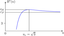
Figure 1: The non-monotonic odd function $H^{\prime}(u)$.

Hence, with decreasing $|c|$ a divergence for $u^{\prime}$ is first encountered for $|c|=c_{M}$. Performing an expansion of (26) up to the first non-trivial order, we find that

$$\rho-\rho_{c}=\frac{1}{6}H^{\prime\prime\prime}(u_{c})(u_{*}-u_{c})^{3}$$ (31)

up to subleading corrections. In the expansion we used (29) and that $H^{\prime\prime}$ vanishes at $u_{c}$. We note that (31) is continuous across $(u_{*},\rho)=(u_{c},\rho_{c})$. Therefore, the non-analyticity in the solution can be written as

$$u_{*}-u_{s}=\mp\,{\rm sgn}(\rho-\rho_{c})\left|\frac{\rho-\rho_{c}}{\frac{1}{6}H^{\prime\prime\prime}(u_{c})}\right|^{1/3}\,,$$ (32)

where the signs refer to $c=\mp c_{M}$, leading to a non-perturbative Landau pole in $u^{\prime}_{*}$,

$$\frac{1}{u^{\prime}_{*}}=\mp\frac{9}{2}\left|H^{\prime\prime\prime}(u_{c})\right|^{1/3}\,\left|{\rho-\rho_{c}}\right|^{2/3}\,.$$ (33)

At a fixed point solution, the Landau pole remains invisible, because it is achieved at the negative $\rho_{c}=-1/8$. Increasing the coupling by lowering $|c|$ below $c_{M}$, the expansion in the vicinity of $d\rho/du=0$ becomes

$$\rho-\rho_{s}=\frac{1}{2}H^{\prime\prime}(u_{s})(u_{*}-u_{s})^{2}$$ (34)

up to subleading terms, where $u_{s}$ is determined through (29). In this regime, $H^{\prime\prime}(u_{s})$ is non-zero throughout. In the parameter range $c_{P}\leq|c|<c_{M}$ we find two solutions for $u_{s}$ with $|u_{s1}|<|u_{c}|<|u_{s2}|$ and $H^{\prime\prime}(u_{s1})<0<H^{\prime\prime}(u_{s2})$. Effectively, the solution for the superpotential becomes multi-valued in a limited region of field space. For $|c|<c_{P}$ we find one solution for $u_{s}$ with $H^{\prime\prime}(u_{s})>0$. In contrast to (33), the non-analyticity has turned into a square root,

$$\frac{1}{u^{\prime}_{*}}=\pm 2\left|H^{\prime\prime}(u_{s})\right|^{1/2}\,\left({\rho-\rho_{s}}\right)^{1/2}\,.$$ (35)

The non-analyticity (35) is stronger than (33) and the solution (34) cannot be continued continuously beyond the point $(u_{*},\rho)=(u_{s},\rho_{s})$. For $|c|<c_{L}$, we have that $\rho_{s}(c)>0$ and the pole appears in the physical regime. In contrast, the solutions extend over all fields provided that $\rho_{s}\leq 0$ which is the case for $|c|\geq c_{L}$.

It is interesting to note that non-analyticities, such as cusps, have been detected previously in the context of the random field Ising model, where disorder is technically introduced with the help of Parisi-Sourlas supersymmetry. Using functional renormalization, it has been argued that a cusp behavior at finite “Larkin scales” $k=k_{L}>0$ is at the origin for the spontaneous breaking of Parisi-Sourlas supersymmetry Tissier:2011zz ; Tissier:2011mu ; Tissier:2011mv .

At this point it should be mentioned that the superpotential $W^{\prime}$ shows another non-analytic behavior: It is not differentiable at its node $\bar{\rho}_{0}$ in the exact IR limit for arbitrary couplings $c>0$. This issue is discussed in detail in Sec. V.2.2 and V.4 below.

IV Renormalized field theory

In this section, we discuss the spontaneous breaking of symmetry and the phase structure of the model in the limit where the UV scale $\Lambda$ is removed.

IV.1 Renormalization

The solution (22) is valid for all $k$ and $\Lambda$, and we may take the ‘continuum limit’ $1/\Lambda\to 0$. The term containing the explicit $t$-dependence drops out in the continuum limit, in consequence of the limit $k/\Lambda\to 0$ for fixed and finite $k$ and (25). The remaining scale-dependence solely reduces to the implicit scale-dependence of $\rho_{0}(k)$ in

$$\begin{array}[]{rl}\rho-\rho_{0}(k)&=c\,{u}+H(u)\\[4.30554pt] \rho_{0}(k)&=1+\bar{\rho}_{0}/k\,.\end{array}$$ (36)

The dimensional parameter $\bar{\rho}_{0}$ has taken over the role of $\delta\kappa\,\Lambda$ in (22). In the above, the VEV (or the mass term, respectively) is the only quantity which is non-trivially renormalized in the continuum limit by requiring that

$$\bar{\rho}_{0}\equiv\lim_{\Lambda\to\infty}(\delta\kappa(\Lambda)\,\Lambda)<\infty\,.$$ (37)

Consequently, the canonical dimension of fields remain unchanged (no anomalous dimension). The continuum limit maps the original set of free parameters $(\tau,\kappa,\Lambda)$ to the parameters $(\tau,\bar{\rho}_{0})$. Note that all couplings of the superfield derivative – the marginal coupling $c$ and the IR attractive higher-order couplings $u^{(n)}(\rho_{0})$ – have settled on their fixed point values. The only ‘coupling’ which has not settled on a fixed point is the UV attractive dimensionless VEV $\rho_{0}$. With this perspective, $\bar{\rho}_{0}$ and the non-renormalized parameter $c$ should be viewed as a free parameters of the model, fixed by the microscopic parameters of the theory. In terms of the dimensional fields $\bar{\rho}=\rho\,k$ and superfield derivative $W^{\prime}(\bar{\rho})=u(\rho)\,k$, the integrated RG flow becomes

$$\begin{array}[]{rl}\bar{\rho}-\bar{\rho}_{0}(k)&=\displaystyle c\,W^{\prime}+kH\left(W^{\prime}\!/k\right)\\[4.30554pt] \bar{\rho}_{0}(k)&=k+\bar{\rho}_{0}\,.\end{array}$$ (38)

We note that $\bar{\rho}_{0}$ also has the interpretation of the physical VEV in the infrared limit of the theory, provided it is positive. Below, we find it is useful to switch between the representations (36) and (38).

IV.2 Characteristic energy

The RG flow (36), (38) carries a characteristic energy scale $E$, meaning that the theory changes its qualitative behavior depending on whether fluctuations have an energy larger or smaller than $E$. The energy scale is set by the UV renormalization of the model (37) and given by

$$E=|\bar{\rho}_{0}|\,.$$ (39)

For $k\gg E$, the dimensionful VEV scales proportional to $k$, and the dimensionless parameter $\rho_{0}$ becomes a constant. This corresponds to a fixed point. All other dimensionless couplings equally have stopped to evolve with RG scale and thus the entire solution approaches a high-energy (UV) fixed point. This fixed point would persist for all $k$ provided that $E=0$. It then has also the interpretation of an IR fixed point. This regime is most conveniently described using (36). For $E>0$, and with decreasing $k$, deviations from the fixed point become visible once $k$ reaches $E$. Here the VEV displays a cross-over from linear scaling $\bar{\rho}(k)\propto k$ for $k\gg E$ to the constant value $\bar{\rho}_{0}$ for $k\ll E$. In full analogy, the dimensionless VEV displays a cross-over from a constant value to scaling inversely proportional to the RG scale. In addition, the running of all dimensionful couplings in the potential is switched on once $k\approx E$ and below. This regime is conveniently described using (38) which governs the remaining RG running through its RHS.

IV.3 Gap equations

Figure 2: Schematic phase diagram of the supersymmetric model based on the gap equation (42) in the infinite cutoff limit. Results agree with earlier findings in Bardeen:1984dx ; Moshe:2003xn .

We first discuss the phase structure based on the integrated RG equations in the IR limit $k=0$, see Fig. 2. This allows for a direct comparison with earlier results based on gap equations and Schwinger-Dyson equations Bardeen:1984dx ; Moshe:2003xn . In the infrared limit we may use (24) in (38) and obtain

$$\bar{\rho}-\bar{\rho}_{0}=c\,W^{\prime}+c_{P}\left|W^{\prime}\right|\,.$$ (40)

Since the potential shows a local minimum at vanishing field, the squared particle masses are given by

$$\bar{\mu}^{2}=\left.V^{\prime\prime}(\phi)\right|_{\phi=0}=\left.W^{\prime\,2}(\bar{\rho})\right|_{\bar{\rho}=0}.$$ (41)

Thus, (40) becomes a gap equation for the mass parameter $\bar{\mu}\equiv W^{\prime}(\bar{\rho}=0)$,

$$\bar{\rho}_{0}=-c\,\bar{\mu}-c_{P}\left|\bar{\mu}\right|\,.$$ (42)

The significance of (42) is as follows. For fixed $\bar{\rho}_{0}$ and $c$ it yields the possible infrared solutions for the masses at vanishing field. Without loss of generality we restrict the discussion to $c\geq 0$. For non-vanishing $\bar{\rho}_{0}$ we find two solutions

$$\begin{array}[]{rl}m\,=\bar{\mu}=&\displaystyle-\frac{\bar{\rho}_{0}}{c_{P}+c}\geq 0\\[8.61108pt] M\!=-\bar{\mu}=&\displaystyle-\frac{\bar{\rho}_{0}}{c_{P}-c}\geq 0\,.\end{array}$$ (43)

In the symmetric regime with negative $\bar{\rho}_{0}$ the mass $m$ is always present and the second mass $M$ is available as long as $c<c_{P}$. In the SSB regime with positive $\bar{\rho}_{0}$ there are two degenerate ground states: As expected, we find a non-symmetric ground state with a radial mass $M_{\rho}$, see sections  V.4 and V.5. However, for $c>c_{P}$, the gap equations show an additional symmetric ground state, characterized by the mass $M$. Note that changing the sign of $c$ leads to equivalent results under the following replacements

$$(c,m,M,M_{\rho})\leftrightarrow(-c,M,m,-M_{\rho})\,.$$ (44)

At the phase transition, i.e. for $\bar{\rho}_{0}=0$, the gap equation (42) states that either $c=\pi$ with the mass $M>0$ undetermined, or $c=-\pi$ and the mass $m$ undetermined. These findings agree with the earlier ones from Bardeen:1984dx ; Moshe:2003xn . The sole difference is that the value for the critical coupling, $c_{P}$, depends on the regularization. The precise link to the conventions used in Bardeen:1984dx ; Moshe:2003xn is given in Tab. 1.

this paper	$\bar{\rho}_{0}$	$\tau=1/c$
Bardeen et. al. Bardeen:1984dx	$-4\pi^{2}{\mu}{\lambda}^{-1}$	$({4\pi^{2}})^{-1}\lambda$
Moshe and Zinn-Justin Moshe:2003xn	$-4\pi^{2}({\mu-\mu_{c}})u^{-1}$	$({4\pi^{2}})^{-1}u$

Table 1: “Translation guide” between the conventions used in Bardeen:1984dx , Moshe:2003xn , and this paper.

IV.4 RG phase diagram

Next we discuss the phase diagram implied by the integrated RG equations for all scales $k$, and compare with the results based on the $k=0$ limit.

IV.4.1 Graphical representation

We begin with a useful graphical representation of the renormalized RG trajectories (36). For vanishing $\bar{\rho}_{0}$, we note that the trajectories (36) reduce to the fixed point solutions $u_{*}(\rho)$ analyzed in Litim:2011bf . The only difference with the fixed point solutions is related to a shift of the argument,

$$u(\rho)=u_{*}(X)\,,\quad X\equiv\rho+1-\rho_{0}(k)=\rho-\frac{\bar{\rho}_{0}}{k}$$ (45)

in terms of the fixed point solutions.

Figure 3: Graphical representation of the solutions $u_{*}(X)$ of (36), where $X=\rho-\bar{\rho}_{0}/k$. The shaded areas are separated by thick lines at $|c|=c_{I},c_{L},c_{P},c_{M}$ and $c_{G}$.

The structure of the solutions and their dependence on the constant $c$ is shown in Fig. 3. Once the free parameters are fixed, the RG evolution of a particular solution stays on a curve with constant $c$, indicated by the curves given in the Figure. Rotating counter-clockwise around $(X,u_{*})=(1,0)$ from the horizontal $c_{G}$-line to the $c_{I}$-curve (from the $c_{I}$-curve to the $c_{G}$-line) covers all curves with positive (negative) $c$. Both sets connect through the point $(1,0)$. We recall that $(c,u_{*})\leftrightarrow(-c,-u_{*})$ describe equivalent physics.

Using (45) and (36), we conclude that for $u(\rho)$ to cover all physical fields $\rho\in[0,\infty]$, we need that

$$X\in\left[-\bar{\rho}_{0}/k,\infty\right]\,.$$ (46)

The curves $u_{*}(X)$ in Fig. 3 define monotonous (and invertible) functions provided that $X>1$. A unique classification of curves is then achieved by choosing a value for $u_{*}$ on a line of constant $X>1$, together with fixing $\bar{\rho}_{0}$. Interestingly, two different values for $u_{*}$ may correspond to one and the same parameter $c$. Below, we mostly stick to the classification in terms of $c$, and we will highlight situations where this is no longer sufficient.

Figure 4: RG trajectories in the $O(N)$ symmetric phase: at weak coupling, trajectories either show a non-vanishing VEV for large scales (SYM, yellow shading), or a vanishing VEV for all scales ($\overline{\rm SYM}$, green shading). At strong coupling trajectories terminate at Landau poles.

Figure 5: RG trajectories $u_{*}(X)$ according to (36) in the regions with spontaneous breaking of the $O(N)$ symmetry in the parametrization (45). Couplings are either finite for all $k$ (SSB, blue shading), or run into a singularity (Landau, red shading). Some trajectories cannot be continued beyond the Landau pole (magenta shading). The SSB phase cannot be defined for strong coupling (white area).

IV.4.2 Symmetric regime

The symmetric phase is characterized by a finite and negative $\bar{\rho}_{0}$ and for large scales $X$ reduces to $\rho$. A restriction on the coupling parameter $c$ is imposed if we require that the solution $u$ should exist for all $\rho$. For weak coupling,

$$\bar{\rho}_{0}<0\,,\quad|c|\geq c_{P}$$ (47)

all $u_{*}$ are single-valued for non-negative arguments such that the $u_{*}(X)$ stay well-defined for all scales, see Fig. 4. For intermediate coupling

$$\bar{\rho}_{0}<0\,,\quad c_{P}\geq|c|\geq c_{L}$$ (48)

the theory admits two distinct effective potentials, and two scalar mass parameters. They are related to trajectories which either run through a node, or not, depending on whether $u(0)$ for $k\gg E$ is larger or smaller than 1, see Fig. 4. The theory is then characterized by the coupling and the scalar mass at vanishing field. This peculiar structure has been found previously and we discuss it in more detail below.

IV.4.3 Symmetry broken regime

Spontaneous symmetry breaking is possible for positive $\bar{\rho}_{0}$. This requires that $u_{*}(X)$ has to be well-defined for all real $X$. In view of the analytical solution in Fig. 3, this limits the achievable couplings to

$$\bar{\rho}_{0}>0,\quad|c|>c_{P}.$$ (49)

Smaller $|c|$ do not lead to a well-defined physical theory in the IR. For

$$\bar{\rho}_{0}>0,\quad|c|\geq c_{M}$$ (50)

the function $u_{*}$ is one-to-one and the theory described by $u(\rho)$ in (36) remains well-defined even in the IR limit. The theory is then characterized by two mass scales. The first one is given by the scalar mass at vanishing field corresponding to an $O(N)$ symmetric phase, whereas the second mass scale is given by the radial mass at $\bar{\rho}=\bar{\rho}_{0}$ allowing for SSB.

IV.4.4 Strong coupling and Landau regime

It remains to discuss the strong coupling and Landau regimes in Figs. 4 and 5. We begin with trajectories in the SYM regime, with

$$\bar{\rho}_{0}<0\,,\quad|c|<c_{L}\,.$$ (51)

We take a ‘bottom-up’ view according to which the couplings evolve from the infrared towards higher scales, parametrizing the effective potential in terms of local couplings in an expansion about vanishing field. Trajectories with (51) emanate from the upper/lower-right corner in Fig. 4 for $k\approx 0$ and increasing $k$ corresponds to decreasing $X$. With increasing $k$, the running mass term and the fermion-boson coupling at vanishing field $u^{\prime}(\rho=0)\equiv u_{*}^{\prime}(-\bar{\rho}_{0}/k)$ diverge at $k=k_{L}$, and the renormalized RG flow comes to a halt: the solutions (36) cannot be continued beyond these points, because $X$ cannot decrease any further along the integral curve $u_{*}(X)$. Interestingly, the potential is double-valued for $k<k_{L}$ with two different trajectories terminating at the same Landau pole. Using (34) together with (45), the non-analyticity in $u$ reads

$$\begin{array}[]{rl}\rho-\rho_{s}(k)&=\frac{1}{2}H^{\prime\prime}(u_{s})(u(\rho)-u_{s})^{2}\end{array}$$ (52)

and the Landau poles are located at

$$\rho_{s}(k)=\rho_{s}-1+\rho_{0}(k)=\rho_{s}+\frac{\bar{\rho}_{0}}{k}\,.$$ (53)

From the fixed point solution we know that $\rho_{s}\leq 1$ and therefore $\rho_{s}(k)\leq\rho_{0}(k)$ for all $k$. In the IR limit, this implies that $\bar{\rho}_{s}(k)\to\bar{\rho}_{0}(k)$ from below. Here, the values for $\rho_{s}$ are fixed by the coupling strength $c$ via (30) and is positive in the regime (51). From (53) it follows that $k_{L}=-\bar{\rho}_{0}/\rho_{s}$ is positive, see Fig. 6. We conclude that the parameters (51) allow for a supersymmetric model with linearly realized $O(N)$ symmetry up to scales $k=k_{L}$.

Figure 6: Location of the UV Landau pole for trajectories in the SYM phase at strong coupling with (51) (see text).

Next we discuss the SSB regime starting with intermediate couplings

$$\bar{\rho}_{0}>0\,,\quad c_{P}\leq|c|\leq c_{M}\,.$$ (54)

Here all curves of constant $c$ contain two Landau points with $|u_{s1}|<|u_{c}|<|u_{s2}|$ and $H^{\prime\prime}(u_{s1})<0<H^{\prime\prime}(u_{s2})$ (see Sec. III.4). Each of them is described by (52) with (53) and parameters $0>\rho_{s2}(c)>\rho_{s1}(c)$. The singularity at $(\rho_{s1},u_{s1})$ corresponds to an IR Landau pole (‘top-down’), whereas the one at $(\rho_{s2},u_{s2})$ corresponds to an UV Landau pole (‘bottom-up’). In the infrared limit, the domain where $u$ is multi-valued, collapses to a point with $\Delta\bar{\rho}=k\,(\rho_{s1}-\rho_{s2})\to 0$. The location of both discontinuities approach the VEV $\bar{\rho}_{s}(k)\to\bar{\rho}_{0}$ from below, and the discontinuity in the superpotential derivative

$$\Delta W^{\prime}\equiv W^{\prime}(\bar{\rho}_{s1})-W^{\prime}(\bar{\rho}_{s2})=k(u_{s1}-u_{s2})$$ (55)

then also becomes arbitrarily small. Interestingly, the UV and IR Landau poles become degenerate on the integral curve for $|c|=c_{M}$ where $\rho_{s1}=\rho_{s2}=-1/8$. The non-analyticity evolves with

$$\begin{array}[]{rl}u(\rho)-u_{s}&\displaystyle=\mp\,{\rm sgn}(\rho-\rho_{s}(k))\left|\frac{\rho-\rho_{s}(k)}{\frac{1}{6}H^{\prime\prime\prime}(u_{s})}\right|^{1/3}\end{array}$$ (56)

together with (53). In this case, the quartic scalar self-coupling $u^{\prime}(\rho=0)$ still diverges at the Landau pole, but the renormalized RG flow continues non-perturbatively rendering $u^{\prime}(0)$ again finite. The non-analyticity (56) first appears for vanishing field at the scale $k_{L}=-\bar{\rho}_{0}/\rho_{s}$ and evolves up to the VEV $\bar{\rho}_{0}$ in the IR limit.

Next we consider the SSB regime at strong coupling,

$$\bar{\rho}_{0}>0\,,\quad|c|<c_{L}\,.$$ (57)

The model has a radial mass proportional to the VEV. Curves of constant $c$ in Fig. 5 have a Landau pole with (52,53) and parameter $\rho_{s}>0$. The integral curves have no continuation beyond the pole, which occurs within the physical regime for all $k$. In particular, the effective potential is not defined for the entire inner part $\bar{\rho}<\bar{\rho}_{0}$ in the IR limit and a scalar mass $W^{\prime}(0)$ cannot be defined.

Finally we consider trajectories in the SSB regime, with

$$\bar{\rho}_{0}>0\,,\quad c_{L}<|c|<c_{P}\,.$$ (58)

Here, in contrast to (57), solutions (45) cover all positive values for $X$ even for large $k$; see (46). In a ‘top-down’ perspective (with decreasing $k$) trajectories in the regime (58) emanate at $X\approx 0$ and continue towards smaller $X$. Again, all trajectories reach a Landau pole for the quartic (and higher) superfield coupling at vanishing field, given by (52) and (53) with the parameter $\rho_{s}(c)$ taking negative values. The Landau scale reads $k_{L}=-\bar{\rho}_{0}/\rho_{s}>0$, and the effective potential does not exist for fields below $\bar{\rho}_{s}(k)=k(\rho_{s}-1)+\bar{\rho}_{0}(k)\leq\bar{\rho}_{0}(k)$. As in (57), the theory still has a radial scalar mass set by the VEV and the quartic coupling, because the one-sided derivative $\frac{dW^{\prime}}{d\bar{\rho}}|_{\bar{\rho}_{0}}$ with $\bar{\rho}\geq\bar{\rho}_{0}$ can be taken for fields larger than the VEV. In turn, a scalar mass at vanishing field cannot be defined. Therefore we conclude that the renormalized RG flow cannot be continued towards the infrared for scales below the Landau scale $k<k_{L}$ for parameters (58).

Figure 7: Schematic phase diagram based on the RG in the infinite cutoff limit. The scale $k_{L}$ is given in Fig. 6. The tighter constraints as opposed to Fig. 2 arise from the inspection of the full effective potential at all scales $k$. The parameter range between $c_{M}$, $c_{P}$ and $c_{L}$ is very narrow (28).

IV.5 Discussion

Our results are summarized in Fig. 7 and should be compared with Fig. 2. The phase diagram is given in dependence on the coupling parameter $c$ and the scale parameter $\bar{\rho}_{0}$.

In the SYM regime, the theory has a weakly coupled phase with a scalar mass $m$ where both the $O(N)$ symmetry and supersymmetry are preserved (47). With increasing coupling parameter $\tau$, the theory admits two $O(N)$ symmetric phases with two mass scales $m$ and $M$ (48). This regime has a very narrow width in parameter space, see (28), which is sensitive to the underlying regularization. For strong coupling (51), the theory displays two mass scales $m$ and $M$. However, it is also plagued by Landau-type singularities which admit no solution for the superpotential at scales above the Landau scale $k_{L}$. This is not visible from an evaluation of the IR gap equations alone, see Fig. 2 for comparison.

In the SSB regime, the theory has a weakly coupled phase (50) where the $O(N)$ symmetry could be spontaneously broken and the effective potential for the scalar has two degenerate minima corresponding to two mass scales $M$ and $M_{\rho}$. The first mass scale is associated with an $O(N)$ symmetric phase, whereas the second mass scale emerges from a finite VEV allowing for SSB. Furthermore, global supersymmetry remains intact. With increasing coupling parameter $\tau$, the theory enters a narrow parameter range where RG trajectories would run through a series of Landau poles at intermediate energies (54). Here, the discontinuity in field space and in the superpotential derivative shrinks to zero in the IR limit, the details of which are sensitive to the underlying regularization. For even larger couplings $|c|<c_{P}$ (57) and (58), the theory is so strongly coupled that RG trajectories terminate at Landau poles in the physical regime. The effective potential does not exist for fields below the non-trivial VEV $\bar{\rho}<\bar{\rho}_{0}$ in the IR limit. Still, the potential does admit a radial mass $M_{\rho}$.

Unbroken global supersymmetry requires a ground state with vanishing energy, and an elsewise positive dimensionful effective potential for all fields and all RG scales. Strictly speaking, the non-existence of an effective potential for small fields means that we cannot decide, based on the potential alone, whether supersymmetry is spontaneously broken at strong coupling, or not. However, the occurrence of a Landau scale $k_{L}$ makes it conceivable that supersymmetry may be spontaneously broken in the strongly coupled regime. This interpretation would be consistent with the picture for the spontaneous breaking of Parisi-Sourlas supersymmetry in disordered Ising models Tissier:2011zz , which is triggered by cusp-like non-analyticities of the RG flow at a finite ”Larkin scale” $k_{L}$. At strong coupling, these limitations of the full effective potential and the occurrence of Landau poles are not directly visible from the infrared limit only, see Figs. 2 and 7. It is a virtue of the fully integrated RG flow for all scales $k$ that the structure of the effective potential at strong coupling has become transparent.

V Effective field theory

In this section we discuss the integrated RG flow from an effective theory perspective. We assume that the UV scale $\Lambda$ is finite, and that the boundary condition at $k=\Lambda$ has been achieved by integrating-out the fluctuations with momenta above $\Lambda$. The RG equations then detail the remaining low-energy flow of couplings for all scales $k<\Lambda$. In terms of dimensional quantities, the solution (22) reads

$$\begin{array}[]{rl}\bar{\rho}-\bar{\rho}_{0}(k)&=\displaystyle c\,W^{\prime}+H\left(\frac{W^{\prime}}{k}\right)\,k-H\left(\frac{W^{\prime}}{\Lambda}\right)\,\Lambda\\[4.30554pt] \bar{\rho}_{0}(k)&=k+\bar{\rho}_{0}\,.\end{array}$$ (59)

The parameter $\bar{\rho}_{0}$ is given by $\bar{\rho}_{0}=\Lambda(\kappa-1)$ in terms of the microscopic (UV) parameters. Our motivation for studying (59) is twofold. Firstly, we want to further clarify the origin of the “peculiar” phases discussed in the previous section. Second, we want to evaluate the effect of changes in the boundary condition and higher-order couplings on the phase structure and critical phenomena

Figure 8: The graphical solution of the gap equation (61) in the symmetric phases with $\bar{\rho}_{0}<0$. For positive $\mu$ there exist one, two or three solutions.

V.1 Gap equations

We begin with the IR limit of the integrated RG flow. The corresponding gap equations for the scalar masses at vanishing field $W^{\prime}(0)\equiv\mu\,\Lambda$, i.e. in the $O(N)$ symmetric phases, are given in terms of the dimensionless parameter $\mu$ by

$$\begin{array}[]{rl}\displaystyle-\frac{\bar{\rho}_{0}}{\Lambda}&=c\,\mu+c_{P}|\mu|-H(\mu).\end{array}$$ (60)

where we used expansion (24) for $H$. For $\bar{\rho}_{0}\neq 0$ we find two possible branches of solutions with

$$\begin{array}[]{rl}H\left(\mu\right)&=\displaystyle(c+c_{p})\mu+\frac{\bar{\rho}_{0}}{\Lambda},\quad(\mu>0)\\[8.61108pt] H\left(\mu\right)&=\displaystyle(c-c_{p})\mu+\frac{\bar{\rho}_{0}}{\Lambda},\quad(\mu<0).\end{array}$$ (61)

We consider $c\geq 0$ since changing the sign amounts to interchanging $\mu\leftrightarrow-\mu$ in (61). The main difference with (42) in the infinite cutoff limit is the appearance of the term $H(\mu)$.

In the SYM regime with negative $\bar{\rho}_{0}$ we find one, two, or three solutions to (61) with $m=\Lambda\mu>0$, and none, one, or two solutions $M=-\Lambda\mu>0$, see Fig. 8. Three solutions for positive $\Lambda\mu$ can only exist if the slope $c+c_{P}$ is inbetween $c_{P}$ and $c_{M}$, cf. Fig. 1.

For most parts of the parameter space we only have a single scalar mass $m$, similar to the weak coupling phase of the renormalized theory. For small $\bar{\rho}_{0}/\Lambda$ and strong coupling, a “triangle” opens up allowing for two additional mass scales of the type $M$. The borderline $c(\bar{\rho}_{0}/\Lambda)$ is found analytically, starting at the point $(c,\bar{\rho}_{0}/\Lambda)=(c_{P},0)$ and ending at $(c,\bar{\rho}_{0}/\Lambda)\approx(0,-1.077)$, see Fig.  9. Furthermore, we find two more masses of the type $m$ in a tiny “spike”-like region at very strong coupling, bordered by the curves connecting $(c,\bar{\rho}_{0}/\Lambda)=(c_{M}-c_{P},-9/8)\approx(0.035,-1.125)$ with $(c,\bar{\rho}_{0}/\Lambda)=(0,-1.077)$ and $(0,-1)$ as indicated in the same Figure.

Figure 9: Phases of the supersymmetric model according to the gap equations at finite UV scale. The SYM phase displays either a single mass scale $m$, or several ones. The SSB regime displays two scalar mass scales $M$ and $M_{\rho}$ for all couplings. Note that the mass scale $M$ represents an $O(N)$ symmetric state within the regime where we would normally only expect SSB to occur. The phase transition between the SYM phase and the SSB phase is continuous with Gaussian exponents.

Figure 10: Phases of the supersymmetric model according to the RG equations at finite UV scale. The SSB regime is quite similar to the result at $1/\Lambda=0$, see Fig 7. The SYM phase is substantially larger (see text). The phase transition between the SYM phase and the SSB phase is continuous with Gaussian exponents. Note that there exists a very tiny Landau phase for couplings $c_{P}<|c|<c_{M}$ in the SSB regime (red line).

The bordering lines $c(\bar{\rho}_{0}/\Lambda)$ are known analytically. In total, we either have a single mass $m$, or three masses $m+2M$ or $3m$, or five different mass scales of the type $3m+2M$ in the region where the triangle and the spike overlap. Some of the masses are parametrically large in the strong coupling domain. We believe that these masses in the very strongly coupled domain are an artifact of the regularisation and should not be trusted.

In the regime $\bar{\rho}_{0}>0$ allowing for SSB, a unique scalar mass solution $M$ to (61) is achieved from the branch with negative $\mu$, for all couplings. In addition, the theory shows the expected radial mass $M_{\rho}$. However, we emphasize that some of the solutions found here, in particular those at strong coupling, have parametrically large masses suggesting that these may be spurious.

V.2 RG phase diagram

Next we turn to the phase diagram of the integrated RG flow at finite $\Lambda$ for all scales $k$.

V.2.1 Symmetric regime

Figure 11: Possible values $W_{L}^{\prime}/\Lambda$ as a function of the inverse superfield coupling coupling $c=1/\tau$ associated with a Landau pole in the IR limit, i.e. with $d\bar{\rho}/dW^{\prime}=0$.

The phase diagram corresponding to (59) is given in Fig. 10, where the axes denote the (inverse) quartic superfield coupling $1/\tau$ and the parameter $\bar{\rho}_{0}$ in units of the initial scale $\Lambda$. For $\bar{\rho}_{0}<0$ the theory is in the symmetric phase, provided that the coupling is small enough. There is also a strong coupling regime where the RG flow develops a Landau pole and the effective potential becomes multi-valued in the physical regime $\bar{\rho}>0$. The boundary between the two regimes is marked by a curve $c_{\rm cr}(\bar{\rho}_{0}/\Lambda)$. The latter is determined as follows: In the IR limit, the solution (59) reads

$$\bar{\rho}-\bar{\rho}_{0}=cW^{\prime}+\pi|W^{\prime}|-H\left(\frac{W^{\prime}}{\Lambda}\right)\Lambda$$ (62)

and shows a Landau pole, if $d\bar{\rho}/dW^{\prime}$ vanishes. Using (62) in the condition $d\bar{\rho}/dW^{\prime}=0$ at $\bar{\rho}=0$ yields

$$\frac{\bar{\rho}_{0}}{\Lambda}=H\left(\frac{W^{\prime}_{L}}{\Lambda}\right)-\frac{W_{L}^{\prime}}{\Lambda}\,H^{\prime}\left(\frac{W_{L}^{\prime}}{\Lambda}\right),$$ (63)

where $W^{\prime}_{L}$ is equal to $W^{\prime}(0)$ when the Landau pole enters the physical region at $\bar{\rho}=0$. The real roots of this polynomial equation are

$$\frac{W_{L}^{\prime}}{\Lambda}=\pm\left(\frac{\sqrt{9+8\bar{\rho}_{0}/\Lambda}-\left(3+2\bar{\rho}_{0}/\Lambda\right)}{2\left(1+\bar{\rho}_{0}/\Lambda\right)}\right)^{1/2},$$ (64)

where the plus (minus) sign belongs to the critical coupling characterizing a Landau pole at $\bar{\rho}=0$ in the positive (negative) half-plane of $W^{\prime}$. Inserting this into (62), evaluated at $\bar{\rho}=0$, yields the critical couplings

$$c_{\rm cr}=\left.\frac{1}{W^{\prime}}\left(-\bar{\rho}_{0}+H\left(\frac{W^{\prime}}{\Lambda}\right)\Lambda-c_{P}|W^{\prime}|\right)\right|_{W^{\prime}_{L}}$$ (65)

as a function of the VEV $\bar{\rho}_{0}$. In general, we find that the occurrence of Landau poles is only possible in the parameter range $\bar{\rho}_{0}/\Lambda\in(-1.125,0)$ and $c\in(0,c_{P})$, i.e. the strong coupling regime. Besides ambiguities with $W_{L}^{\prime}<0$ for couplings $c<c_{P}$, we also find Landau poles with $W_{L}^{\prime}>0$ in the very narrow strong coupling regime with $c<(c_{M}-c_{P})\approx 0.035$, see Fig. 11.

Hence, we interpret the different regimes of the symmetric phase as follows (see Fig. 10): We observe Landau poles in the physical regime with $W_{L}^{\prime}<0$, if the superfield coupling $\tau$ is larger than $c^{-1}_{\rm cr-}$, i.e. $c<c_{\rm cr-}$. The corresponding borderline starts at the point $(c,\bar{\rho}_{0}/\Lambda)=(c_{P},0)$ and ends at $(0,-1.077)$, similar to borderline resulting from the gap-equation analysis. Furthermore, for very strong couplings $c<c_{M}-c_{P}\ll 1$ we observe ambiguities with $W_{L}^{\prime}>0$ in the physical regime (dark shaded area in Fig. 10). However, this area is bounded by $c_{\rm cr+}$ from below, where $c_{\rm cr+}$ starts at $(c_{M}-c_{P},-1.125)$ and ends at $(0,-1.077)$.

Interestingly, the available domain of couplings is substantially larger than in Fig. 7. The reason for that is quite intuitive, since decreasing the VEV $\bar{\rho}_{0}$ comes along with a shift of the solution $W^{\prime}$ to the left and thus the Landau pole may enter the unphysical regime $\bar{\rho}<0$. In addition, the equations do not admit a second mass $M$, unlike the case for $1/\Lambda=0$. We emphasize that the RG study of the phase diagram also allows for a simple descriptive explanation of the occurrence of the various masses as shown in Fig. 9. The two additional masses $M$, observed in the strong coupling domain (see big triangle, Fig. 9) result from an ambiguity of the solution $W^{\prime}$ in the negative half-plane. The borderline connecting $(c_{P},0)$ and $(0,-1.077)$ in Fig. 9 represents the special solution with $c=c_{cr-}$ showing a Landau pole in the IR exactly at $\bar{\rho}=0$ and this corresponds to an additional infinitely large mass $M$. Similarly, the two additional masses of type $m$ in the spike-like strong coupling region result from ambiguities of the solution for positive $W^{\prime}$.

V.2.2 Symmetry broken regime

For $\bar{\rho}_{0}>0$, the theory is in a phase featuring spontaneous $O(N)$ symmetry breaking. For sufficiently weak coupling with $|c|\geq c_{M}$, the theory displays a well-defined low-energy regime with two mass scales $M$ and $M_{\rho}$. The first one is associated to the curvature at vanishing field and thus represents an $O(N)$ symmetric phase, whereas the second mass is given by the curvature at the non-vanishing VEV $\rho_{0}$ and implies SSB.

Figure 12: Effective field theory with finite $\Lambda$: Graphical representation of the dimensionless superpotential derivative $u(X)$ as a function of $X=\rho-\bar{\rho}_{0}/k$ in (45) for weak, intermediate and strong superfield coupling (from left to right). Each panel shows the RG flow, starting with $u_{\Lambda}(\rho)=\tau\left(\rho-\rho_{0}(\Lambda)\right)$ according to (19) in the UV up to the IR limit.

In the very narrow coupling-regime $c_{P}<|c|<c_{M}$ there occur IR Landau poles at $(\rho_{s}(k),u_{s}(k))$ with

$$\rho_{s}(k) =1+c\,u_{s}+H(u_{s})-H\left(u_{s}e^{t}\right)e^{-t}+\frac{\bar{\rho}_{0}}{k},$$

$$0 =c+H^{\prime}\left(u_{s}\right)-H^{\prime}\left(u_{s}e^{t}\right)$$ (66)

within the physical regime for scales $k<k_{L}$. However, similar to the renormalized theory, the poles approach the VEV $\lim_{k\rightarrow 0}\bar{\rho}_{s}(k)\rightarrow\bar{\rho}_{0}$ in the IR limit from below and the domain, where $W^{\prime}$ is multi-valued collapses to a point. Hence, the effective Potential is well defined and unique.

For stronger couplings $c<c_{P}$, the effective potential is plagued by Landau poles and becomes multi-valued even in the IR. This becomes apparent by considering the second derivative $W^{\prime\prime}$ of the superpotential. The latter shows a non-analyticity at $\bar{\rho}_{0}$ exactly in the IR limit with

$$\lim_{\;\bar{\rho}\rightarrow\bar{\rho}_{0\pm}}W^{\prime\prime}(\bar{\rho})=\frac{1}{c\pm\pi},$$ (67)

where $W^{\prime}(\bar{\rho}_{0\pm})\rightarrow\pm 0$. Apparently, the solution $W^{\prime}$ shows a cusp with positive $W^{\prime\prime}$ for $W^{\prime}\rightarrow+0$ and negative $W^{\prime\prime}$ for $W^{\prime}\rightarrow-0$ in the vicinity of the node if $|c|<c_{P}$. Since there exists at most one Landau pole with $W^{\prime}_{L}<0$ in the IR limit (Fig. 11) and since $W^{\prime}(\bar{\rho}\rightarrow-\infty)=-\infty$, it becomes apparent that there has to be a Landau pole located in the physical regime for $k\rightarrow 0$ if and only if $|c|<c_{P}$.

V.3 Discussion

Now we compare and discuss the phase diagrams obtained by (a) considering the renormalized theory with $\Lambda\rightarrow\infty$ and (b) looking at the effective theory with $\Lambda$ finite.

Firstly, let us compare the phase diagrams Fig. 2 and 9 as derived from the gap equations (42) and (61). Apparently, the gap equations (61) of the effective theory contain an additional, cutoff (and regulator)-dependent contribution $H(\mu)$ compared to (42). The term $H(\mu)$ thus leads to the following modifications of the phase diagram of the renormalized theory: In the symmetric phase, it diminishes the parameter-range where we observe further masses in addition to $m$. Besides, we find up to five different $O(N)$ symmetric phases in the very strong-coupling regime $|c|\ll 1$ and for certain VEV $\bar{\rho}_{0}$. In the spontaneously broken regime, the function $H(\mu)$ enlarges the parameter range to infinitely large couplings $\tau=1/c$, where we observe a second mass $M$ in addition to $M_{\rho}$. However, since the masses in the very strong coupling regime are quite large, i.e. of the order of the cutoff $\Lambda$, we believe them to be regulator-dependent and unphysical.

Figure 13: Effective field theory with finite $\Lambda$: Graphical representation of the dimensionful superpotential derivative $W^{\prime}/\Lambda$ as a function of $\bar{X}=\left(\bar{\rho}-\bar{\rho}_{0}\right)/\Lambda$ for weak, intermediate and strong superfield coupling (from left to right). Each panel shows the RG flow of the superpotential, starting with $W^{\prime}_{\Lambda}(\bar{\rho})=\tau\left(\bar{\rho}-\bar{\rho}_{0}(\Lambda)\right)$ according to (19) in the UV up to the IR limit. Note the non-analyticity of the effective superpotential at $\bar{X}=0$ in the IR limit $k\rightarrow 0$ (see Secs. V.2.2 and V.4). Note further that the running potential with $c=c_{P}$ (middle panel) shows ambiguities for very small $|\bar{X}|\ll 1$ for small scales $k$ which are not visible in the figure.

Next, let us compare the phase diagrams Fig. 7 and 10 as deduced from our RG studies. Here, we claimed solutions $W^{\prime}(\bar{\rho})$ to be physically relevant, if there exists no Landau pole characterized by an infinitely large fermion-boson coupling $W^{\prime\prime}$ in the physical domain.

Let us first consider the SYM regime. Here, the narrow window between the couplings $c_{L}$ and $c_{P}$, where there exist two masses $m$ and $M$ vanishes for finite $\Lambda$ and the effective theory shows only a single mass $m$. Furthermore, the strong coupling domain is reduced and becomes $\bar{\rho}_{0}$-dependent for $\Lambda$ finite. The different structure of the SYM regimes become apparent by comparing Fig. 3 with Fig. 12, 13. In the renormalized theory (Fig. 3), there exists an UV Landau pole in the physical domain for superfield couplings stronger than $\tau=c_{L}^{-1}$ and the potential is not even defined for all fields $\rho>0$. In contrast, the effective theory always features a well-defined UV limit, given by the superpotential $W^{\prime}_{\Lambda}=\tau\left(\bar{\rho}-\bar{\rho}_{0}(\Lambda)\right)$ at the UV scale $k=\Lambda$. The potential is defined for all fields but may show ambiguities for sufficiently strong couplings. This is illustrated in Fig. 13, where the superpotential $W^{\prime}/\Lambda$ is plotted as a function of $\bar{X}=\left(\bar{\rho}-\bar{\rho}_{0}\right)/\Lambda$. In the SYM phase, the origin $\bar{\rho}=0$ corresponds to $\bar{X}=|\bar{\rho}_{0}|/\Lambda>0$. Now, let us consider the strongly coupled domain with $|c|<c_{P}$ fixed (Fig. 13, right panel) and $|\bar{\rho}_{0}|\ll 1$. Here, a IR Landau pole occurs at $k_{L}>0$ in the physical regime and additional masses at the origin appear by approaching the IR. However, if we choose $|\bar{\rho}_{0}|$ large enough, the IR Landau pole drifts out of the physical domain and the effective potential is unique and well-defined for all $\bar{\rho}\geq 0$ with a single mass $m$. This upper limit of $|\bar{\rho}_{0}|(c)$ simply corresponds to the borderline connecting $(c_{P},0)$ and $(0,-1.077)$ in Fig. 10.

We find identical weak, Landau and strong coupling SSB regimes for the renormalized and the effective theory, see Fig. 7, 10. The renormalized as well as the effective theory exhibit an IR Landau pole for all $|c|<c_{P}$ (Fig. 3 and Fig. 13). The existence of an IR Landau pole within the effective theory is shown as follows, see Fig. 13, right panel: The origin $\bar{\rho}=0$ corresponds to $\bar{X}=-\bar{\rho}_{0}/\Lambda<0$ and thus there always emerges an IR Landau pole in the physical domain at $k_{L}>0$ for $|c|<c_{P}$. Independent of the superfield coupling and the VEV $\bar{\rho}_{0}>0$, there always exists only a single mass $M$ at the origin representing an $O(N)$ symmetric phase. Again, the effective potential is always defined for all fields, but may show ambiguities, whereas the potential is not defined for all fields $\bar{\rho}>0$ in the strong coupling regime $|c|<c_{P}$ in the infinite cutoff-limit $\Lambda\rightarrow\infty$.

Figure 14: Green, solid lines: mass scales $m$, $M$ of the renormalized theory ($\Lambda\rightarrow\infty$) as functions of the coupling $c$ according to the gap equations (43) for fixed $\bar{\rho}_{0}=\{-0.5,-0.5,0.5\}$ (left, middle, right panel). Blue, dashed lines: Masses $m/\Lambda$, $M/\Lambda$ of the effective theory ($\Lambda<\infty$) as functions of the coupling $c$ according to the gap equations (60) for fixed $\bar{\rho}_{0}/\Lambda=\{-0.5,-0.5,0.5\}$.

Finally, Fig. 14 compares the different mass scales of the renormalized and the effective model. Notice that these masses represent $O(N)$ symmetric phases of the model, since they emerge from the curvature of the potential at vanishing field $\bar{\rho}=0$. The parametrically large masses $m$ observed in the spike-like region (see Fig. 9) are not included in Fig. 14, since we believe them to be an artifact of the chosen regularization.

In summary, in the SSB phase, and in the symmetric phase at weak coupling, the difference between the $(\Phi^{2})^{2}_{d=3}$ theory at finite and infinite UV cutoff is minute, resulting in equivalent phase diagrams. In the symmetric phase for $c<c_{P}$, the difference is more pronounced: At finite UV cutoff the fluctuations of the Goldstone modes have less “RG time” available to built-up non-analyticities in the effective potential. This leads to a shift in the effective boundary between weak and strong coupling, allowing for a substantially larger domain of a regular $O(N)$ symmetric phase. At strong coupling, we also conclude that the absence of an $O(N)$ symmetric phase at infinite cutoff arises from the theory at finite UV scale through an $O(N)$ symmetric phase with anomalously large mass of the order of the UV scale itself.

V.4 Effective potential

As already mentioned in Sec. III.2, the relevant microscopic coupling $\kappa=\kappa_{\rm cr}+\bar{\rho}_{0}/\Lambda$ determines the macroscopic physics of the model: if $\kappa<\kappa_{\rm cr}$ ($\bar{\rho}_{0}<0$), the effective potential preserves global $O(N)$ symmetry. Contrary, if $\kappa>\kappa_{\rm cr}$ ($\bar{\rho}_{0}>0$), the symmetry may be spontaneously broken, if the VEV $\bar{\rho}_{0}>0$ is taken. The specific UV coupling $\kappa_{\rm cr}=1$ marks the phase transition between the two regimes. Fig. 15 shows the flow of the effective average potential $V_{k}(\bar{\rho})$ for different values of $\kappa$, starting in the UV at $k=\Lambda$ with

$$V_{\Lambda}=\bar{\rho}\left(W^{\prime}_{\Lambda}\right)^{2}=\tau^{2}\bar{\rho}\left(\bar{\rho}-\kappa\Lambda\right)^{2}$$ (68)

according to (19), up to the IR limit $k\rightarrow 0$. Three aspects of the potential need to be discussed further:

Firstly, there exists a strong coupling domain, where the effective potential shows ambiguities within the physical domain, both in the infinite cutoff limit (Fig. 3) and in the effective theory limit (Fig. 13, right panel). At strong coupling, the effective potential admits no physical solution for small fields, except for an unphysical one with $1/|u^{\prime}|\ll 1$ in the effective theory description. This result indicates that a description of the theory in terms of an effective superpotential is no longer viable, possibly hinting at the formation of bound states with or without the breaking of supersymmetry. Incidentally, for the same parameter values the effective potential admits two solutions for large fields, except for an unphysical third solution one in the effective theory description. The theory admits two different effective potentials associated to the same microscopic parameters, which has been discussed in Litim:2011bf in the context of fixed point solutions.

Secondly, the effective potential at $k=0$ is non-analytic at its nontrivial minimum $\bar{\rho}_{0}$. Consider therefore the second derivative of the superpotential

$$W^{\prime\prime}\left(\bar{\rho}\right)=\frac{1}{c+H^{\prime}\left(W^{\prime}/k\right)-H^{\prime}\left(W^{\prime}/\Lambda\right)}$$ (69)

in the vicinity of $\bar{\rho}_{0}(k)$, where $W^{\prime}(\bar{\rho}_{0}(k))=0$ according to (59). By approaching the IR, (69) simplifies to (67). Apparently, this non-analyticity does not appear until the exact IR limit $k=0$ is approached. Contrary, for all finite scales $k>0$ we find $W^{\prime\prime}(\bar{\rho}_{0}(k))=1/c$, which simply represents the exactly marginal superfield coupling $\tau$. Since the radial mass is given by

$$M_{\rho}^{2}=\left.V^{\prime\prime}(\phi)\right|_{\phi=\phi_{0}}=\left(2\bar{\rho}W^{\prime\prime}(\bar{\rho})\right)^{2}\big{|}_{\rho_{0}(k)},$$ (70)

a uniquely defined radial mass only exists for finite scales $k>0$ and reads

$$M_{\rho}(k)=2\tau\bar{\rho}_{0}(k)=2\tau(k+\bar{\rho}_{0}),\quad\quad\bar{\rho}_{0}>0.$$ (71)

First studies at finite $N$ indicate that the non-analyticity of $W^{\prime}$ for $k=0$ is solely due to the large-$N$ limit.

Thirdly, the effective scalar field potential in the SSB phase with non-vanishing VEV is not convex, even in the IR limit $k\rightarrow 0$. As it has already been mentioned in Synatschke:2008pv , the supersymmetric analogon of the potential term in the classical action is the superpotential $W$, (2). Consequently, a flow of the superpotential is derived which drives the approach to convexity of the superpotential $W$, but not necessarily of the potential $V=\bar{\rho}\,W^{\prime 2}$. The superpotential $W$ is a convex function if and only if the first derivative $W^{\prime}(\bar{\rho})$ represents a monotonically increasing function of $\bar{\rho}$. According to (62), this condition is satisfied as long as $c>c_{P}$, i.e. in the weakly coupled domain. This fact supports the conjecture that supersymmetry may be broken spontaneously in the strongly coupled domain exhibiting Landau poles.

Figure 15: RG flow of the effective average potential $V_{k}/\Lambda^{3}$ as a function of $\bar{\rho}/\Lambda$ according to (59) for different values of $\delta\kappa=\bar{\rho}_{0}/\Lambda=\{-0.1,0,+0.1\}$ at weak coupling $c=3.7$. If $\bar{\rho}_{0}<0$, the system evolves into an $O(N)$ symmetric phase (left panel). Vanishing $\bar{\rho}_{0}$ corresponds to the phase transition between the $O(N)$ symmetric and the SSB phase and the scale invariant solution is approached in the IR limit (middle panel). If $\bar{\rho}_{0}>0$, the macroscopic theory is characterized by a non-vanishing VEV $\bar{\rho}_{0}(k\rightarrow 0)=\bar{\rho}_{0}>0$ (right panel). The insets show the potential at small fields approaching the IR limit.

V.5 Phase transition & critical exponents

The supersymmetric $O(N)$ model in $d=3$ is an effective field theory that features the large-distance properties of statistical models near a second order phase transition. According to Litim:2011bf , the fixed-point solution characterizing the phase transition shows Gaussian scaling for all finite couplings $c$, except for $|c|=c_{P},c_{I}$. Following Berges:2000ew we can also extract the thermodynamical critical exponents. The expectation value of the field $\langle\phi\rangle$ serves as order parameter, and in the SSB regime it is related to the VEV $\bar{\rho}_{0}$ via (choose $\phi_{i}=\delta_{i1}\phi$)

$$\langle\phi\rangle=\lim_{k\rightarrow 0}\sqrt{2\bar{\rho}_{0}(k)}\equiv\sqrt{2\bar{\rho}_{0}}=\sqrt{2\delta\kappa\Lambda}.$$ (72)

We may associate the deviation of $\kappa$ from its critical value $\kappa_{cr}=1$ with the deviation of the temperature $T$ from the critical temperature $T_{c}$ according to $\delta\kappa\Lambda\sim(T_{c}-T)$. Thus we have

$$\langle\phi\rangle\sim\left(\bar{\rho}_{0}\right)^{\beta}\quad\mbox{with}\quad\beta=\frac{1}{2}\,.$$ (73)

Next, consider the critical exponent $\nu$ describing the manner in which the correlation length $\xi$ diverges (the mass vanishes) by approaching the phase transition. We thereby distinguish between

$$\xi^{-1} =m\sim\left(-\bar{\rho}_{0}\right)^{\nu}\quad(\mbox{SYM regime},\,\bar{\rho}_{0}<0)$$

$$\xi^{-1} =m\sim\left(\bar{\rho}_{0}\right)^{\nu^{\prime}}\quad\;\;(\mbox{SSB regime},\;\,\bar{\rho}_{0}>0).$$ (74)

Let’s consider first the squared masses corresponding to $O(N)$ symmetric ground states as given by (41). We are interested in how the superpotential $W^{\prime}$ vanishes at the origin when $\bar{\rho}_{0}\rightarrow 0$. We begin with the parameter range $c>0$ and $c\neq c_{P}$. Using (62) and (25) we have

$$\bar{\rho}-\bar{\rho}_{0}=c\,W^{\prime}+\pi|W^{\prime}|-\frac{3}{\Lambda}W^{\prime\,2}+\mathcal{O}\left(\frac{W^{\prime\,4}}{\Lambda^{3}}\right)$$ (75)

for small masses. In the SYM regime, this gives (43) for $W^{\prime}/\Lambda\ll 1$, where the second mass in (43) only exists in the strong coupling region $c<\pi$. Hence, according to (74) we have

$$\nu=1\,.$$ (76)

In the SSB regime, there exists a unique $O(N)$ symmetric ground state with mass $M$ given by (43) for all $c>\pi$, implying

$$\nu^{\prime}=1\,.$$ (77)

We also observe a spontaneously $O(N)$ broken ground state, characterized by its radial mass according to (71). Since $M_{\rho}\sim\bar{\rho}_{0}$, this also leads to (77).

Now consider the exponent $\delta$, given by $\left.J\right|_{\bar{\rho}_{0}=0}\sim\phi^{\delta}$, where $J=\partial V/\partial\phi$. Close to the phase transition, where we may assume the cutoff to be much larger than the mass scale, i.e. $W^{\prime}/\Lambda\ll 1$, the effective potential reads

$$V(\bar{\rho})=\frac{1}{A^{2}}\,\bar{\rho}\left(\bar{\rho}-\bar{\rho}_{0}\right)^{2}$$ (78)

with $A=c+\pi\operatorname{sgn}(\bar{\rho}-\bar{\rho}_{0})$ and $\operatorname{sgn}(0)=0$. This leads to

$$\left.J\right|_{\bar{\rho}_{0}=0}=\frac{3}{4A^{2}}\phi^{\delta}\quad{\rm with}\quad\delta=5\,.$$ (79)

Finally, we discuss the critical exponent $\gamma$ associated with the susceptibility $\chi=\partial\phi/\partial J=(\partial^{2}V/\partial\phi^{2})^{-1}$ near the phase transition,

$$\left.\chi(J)\right|_{J=0} \sim(-\bar{\rho}_{0})^{\gamma}\quad(\mbox{SYM phase},\,\bar{\rho}_{0}<0)$$

$$\left.\chi(J)\right|_{J=0} \sim(\bar{\rho}_{0})^{\gamma^{\prime}}\quad\,\;(\mbox{SSB phase},\;\;\bar{\rho}_{0}>0).$$ (80)

Using (78) and (80) we get

$$\gamma=\gamma^{\prime}=2\,.$$ (81)

Note that the results (76), (77), (79) and (81) are invariant under changing $c\leftrightarrow-c$, see (44). The thermodynamical scaling exponents derived here can equally be obtained from the leading RG exponent together with scaling relations by using $\nu=1/\theta$, where $\theta=1$ is the IR relevant eigenvalue due to the VEV. The scaling exponents in the special case where $c=\pm c_{P}$ are discussed in the following section.

VI Spontaneous breaking of scale invariance

In this section we discuss the supersymmetric analogon of the Bardeen-Moshe-Bander (BMB) phenomenon, the spontaneous breaking of scale invariance and the associated non-classical scaling.

VI.1 Bardeen-Moshe-Bander phenomenon

We first recall the BMB phenomenon for scalar $O(N)$ symmetric theories. Linear $O(N)$ models serve as perfect testing ground for studying critical phenomena. For large $N$ the solvable spherical model gives a qualitatively accurate picture of the phase structure of the theory. The $(\phi^{2})^{2}_{d=3}$ theory exhibits an IR-attractive Wilson-Fisher fixed point corresponding to a second order phase transition between the $O(N)$ symmetric and the spontaneously broken phase Tetradis:1995br . In contrast, the scalar $(\phi^{2})^{3}_{d=3}$ model shows a more complex phase structure David:1984we ; David:1985zz ; Bardeen:1983rv ; Tetradis:1995br . Depending on the renormalized couplings $\mu^{2},\lambda$ and $\eta$ of the operators $\phi^{2},\phi^{4}$ and $\phi^{6}$, one observes a first-order phase transition without universal behavior or a second-order phase transition with universal behavior. Both regimes are separated by a tricritical line $t$, characterized by vanishing couplings $\mu^{2}$ and $\lambda$ as depicted in Fig. 16. A surface of first-order transitions continues into the $O(N)$ symmetric phase for couplings with $\eta>\eta_{c}$ and ends at a gas-liquid transition line $l$. Scale invariance is an exact symmetry of the tricritical theory, but at the end point $(0,0,\eta_{c})$, scale invariance is spontaneously broken. The free coupling $\eta$ is dimensionally transmuted to an undetermined mass scale $m$ and a massless Goldstone-boson (dilaton) shows up. In the large-$N$ limit this non-trivial and UV-stable BMB fixed-point marks the point where the tricritical line $t$ and the gas-liquid line $l$ meet. Hence, the tricritical line connects the Gaussian fixed point and the BMB fixed point. One expects that at finite $N$ the tricritical line extends all the way to infinite $\eta$ and the BMB point disappears Karsch:1987uj . We note that the BMB fixed point is also of interest as a fundamental UV fixed point, allowing for a non-Gaussian continuum limit for the $(\phi^{2})^{3}_{d=3}$ theory with non-classical scaling.

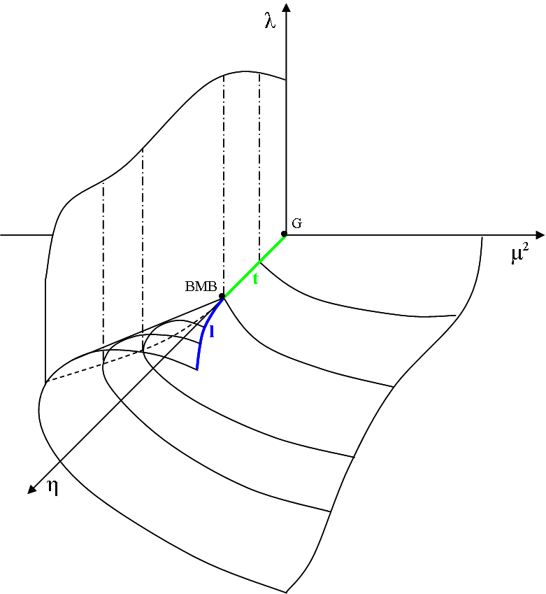
Figure 16: Phase structure of the scalar $O(N)$ model at infinite $N$ including the BMB fixed point, according to David:1985zz (see text).

VI.2 Supersymmetric BMB phenomenon

In the supersymmetric theory, the BMB phenomenon has first been discussed in Bardeen:1984dx with variational methods. Here, the critical $(\Phi^{2})^{2}_{d=3}$ theory with a quartic superfield potential corresponds, in the scalar sector, to a critical $(\phi^{2})^{3}_{d=3}$ with a sextic potential. The main new addition due to supersymmetry is that the scalar quartic and sextic couplings are no longer independent of each other.

Using the fully integrated RG flow, the following picture for the BMB phenomenon emerges: If we fine-tune the classical coupling $\kappa=\kappa_{\rm cr}$, the solution (22) at the origin $\rho=0$ reads

$$-1=c\,u_{0}+H\left(u_{0}\right)\,$$ (82)

in the IR limit, where $u_{0}\equiv u(\rho=0)$. This equation simply represents the fixed point solution at vanishing field. The $O(N)$ symmetric ground state is characterized by the mass

$$M^{2}=\left(W^{\prime}(0)\right)^{2}=\bar{\mu}^{2}=\left(u_{0}\,k\right)^{2},$$ (83)

where $M=-\bar{\mu}>0$. Evidently, $u_{0}$ has to diverge as $1/k$ in order to allow for spontaneous breaking of scale invariance with a finite mass scale $M$ in the IR limit $k\rightarrow 0$. Now we find the transcendental equation (82) to have always a single zero mass solution $M=0$, except for $c=c_{P}$, where it shows an additional, infinitely large solution $u_{0}\to-\infty$. Note that this limit emerges from $u(\rho)$ through negative field squared values $\rho\to 0^{-}$, which is a consequence of our regularisation. Hence, the specific microscopic parameters

$$(\kappa,\tau)=(1,1/\pi)$$ (84)

lead to a macroscopic theory, where the mass of the $O(N)$ bosonic and fermionic quanta is left undetermined. Thus, scale invariance is spontaneously broken in accordance with Bardeen:1984dx ; Moshe:2003xn ; Gudmundsdottir:1984yk and a mass is generated by dimensional transmutation. The coupling parameter $\tau$ takes the value (84) in our conventions, and the associated degree of freedom is ‘transmuted’ to an arbitrary mass scale $M$. Spontaneously broken scale invariance leads to the appearance of a Goldstone boson (dilaton) which is accompanied by a Goldstone fermion (dilatino), since supersymmetry is left unbroken. Note that these particles are exactly massless, since $\tau$ is not renormalized.

VI.3 BMB scaling exponents

Next we turn to the scaling exponents of the supersymmetric BMB fixed point. The critical exponents (74) and (80) become double-valued due to a different scaling behavior of the different mass scales $m,M$ near the fixed point. These, in turn, originate from the finite and the infinite $u_{0}$ solutions detected at $|c|=c_{P}$, see Fig. 3. The latter is responsible for the special nonanalytic behavior of the solution at the BMB fixed point. We first consider $c=c_{P}$, and the critical exponents $\nu$ and $\nu^{\prime}$ defined in (74). By approaching the phase transition from the SYM regime, we find $m=-\bar{\rho}_{0}/2\pi$ and hence

$$\nu=1\,.$$ (85)

In turn, approaching the fixed point from the SSB regime, the expression for $M$ in (43) is not applicable since the contribution linear in $W^{\prime}$ in (75) vanishes. The subleading quadratic terms take over and we are lead to $M^{2}=\frac{\Lambda}{3}\bar{\rho}_{0}$, implying that the supersymmetric BMB exponent $\nu^{\prime}$ is given by

$$\nu_{{}{\rm BMB}}=\frac{1}{2}\,.$$ (86)

We now consider $c=-c_{P}$. By virtue of the symmetry (44) we note that the mass scales $m\leftrightarrow M$ interchange their roles under $c_{P}\leftrightarrow-c_{P}$. Consequently, the scaling exponents (85) and (86) also interchange their values. Therefore we conclude that the theory at $|c|=c_{P}$ displays conventional scaling with (85) as well as un-conventional scaling with (86). The former is a consequence of the smooth ‘non-BMB-type’ scaling related to finite $u_{0}$, whereas the latter is the BMB scaling associated to infinite $u_{0}$. In either case, and under the above identification, we conclude that the scaling indices from the symmetric and symmetry broken regimes agree. We also stress that the BMB scaling exponent (86) is non-classical. Furthermore, it cannot be derived from the RG scaling alone, as they are due to non-analyticities in the field dependences. As a final comment we note that an infinite $u_{0}$, the fingerprint for spontaneous breaking of scale invariance, is stable under alterations of the RG scheme.

VII Radial mode fluctuations

In this section, we give a first account of the phase transition in a theory with finitely rather than infinitely many supermultiplets $N$, focussing on the existence of a fixed point, the phase transition, and the fate of the supersymmetric BMB phenomenon to leading order in a gradient expansion.

VII.1 Exact fixed point

The main new addition to the supersymmetric RG flow at finite $N$ are the fluctuations of the radial mode. They imply that the quartic coupling $\tau$ is no longer an exactly marginal coupling with an identically vanishing $\beta$-function. Instead, the flow of this coupling is governed by terms of order $1/N$. The absence of an exactly marginal coupling implies that the line of fixed points found at infinite $N$ will collapse into a finite, possibly empty set of fixed points. Furthermore, the running of the VEV no longer factorizes from the other couplings of the theory resulting in a more complex structure of the RG flow.

In order to study the supersymmetric $O(N)$ model at finite $N$ we return to the full RG flow (15), which in terms of $u\equiv w^{\prime}$ takes the form

$$\partial_{t}u= -u+\rho\,u^{\prime}-(1-\frac{1}{N})u^{\prime}\,\frac{1-u^{2}}{(1+u^{2})^{2}}$$

$$-\frac{1}{N}(3u^{\prime}+2u^{\prime\prime}\rho)\frac{1-(u+2\rho u^{\prime})^{2}}{(1+(u+2\rho u^{\prime})^{2})^{2}}\,.$$ (87)

A global, analytical, solution of the RG flow (87) is presently not at hand, and we have to resort to approximate solutions instead Bervillier:2007rc . We start with a polynomial approximation to order $n$ for the ‘potential’ $u$, writing

$$u(\rho,t)=\sum_{i=1}^{n}a_{i}(t)(\rho-\rho_{0}(t))^{i}\,.$$ (88)

It expresses the potential in terms of $(n+1)$ couplings $(\rho_{0},a_{1},\cdots,a_{n})$ to determine its fixed points. Inserting the ansatz (88) into the PDE (87) we find a tower of ordinary, coupled differential equations for the couplings,

$$\partial_{t}\rho_{0}(t) =-\rho_{0}(t)+\left(1-\frac{1}{N}\right)$$

$$\,+\frac{1}{N}\left(3+4\rho_{0}(t)\frac{a_{2}(t)}{a_{1}(t)}\right)\frac{(1-(2\rho_{0}(t)a_{1}(t))^{2})}{(1+(2\rho_{0}(t)a_{1}(t))^{2})^{2}}$$

$$\vdots$$

$$\partial_{t}a_{n}(t) =f_{n}\left(\rho_{0}(t),a_{1}(t),a_{2}(t),\cdots,a_{n+2}(t)\right).$$ (89)

Note that the functions $f_{n}$ depend on the couplings $a_{n+1}$ and $a_{n+2}$, because the RHS of (87) involves up to second derivatives of $u$. The fixed point solution requires the flow of all couplings to vanish and hence we set the LHS of (89) equal to zero, leading to an algebraic system of $(n+1)$ equations for $(n+3)$ unknowns. These may be solved, tentatively, by setting the last two couplings $a_{n+1}$ and $a_{n+2}$ to zero. We find

$$\rho_{0*}(N) =1-\frac{1}{N}$$

$$a_{1\,*}(N) =\frac{1}{2}\frac{N}{N-1}$$

$$a_{2\,*}(N) =-\frac{3}{8}\frac{N^{2}}{(N-1)^{2}}$$ (90)

for the first three couplings. The solution bifurcates into two independent fixed points starting with $a_{3}$. Intriguingly, the recursive relation leads to an exact analytical solution of the full system for all $N$ to arbitrarily high expansion order $n$. The reason for this unlikely outcome is that the fixed point (90) is independent of the boundary condition which we have imposed initially on the higher order couplings. This follows from noticing that all fixed point equations (89) with $n\geq 2$ are of the form

$$0 = f_{n}(\rho_{0},a_{1},\dots,a_{n+2})$$

$$= \tilde{f}_{n}(\rho_{0},a_{1},\dots,a_{n})$$

$$\;+\,(n+1)\left(\rho_{0}-1+1/N+\partial_{t}\rho_{0}\right)a_{n+1}$$

$$\;-\,\frac{n+1}{N}\frac{1-\xi^{2}}{(1+\xi^{2})^{2}}\left[(3+2n)a_{n+1}+2(n+2)\rho_{0}a_{n+2}\right]$$

$$\;-\,\frac{4\rho_{0}\xi(n+1)^{2}}{N}\frac{(3a_{1}+4a_{2}\rho_{0})(\xi^{2}-3)}{(1+\xi^{2})^{3}}a_{n+1}\,.$$

Here $\xi=2a_{1}\rho_{0}$, and $\partial_{t}\rho_{0}$ is given according to (89). At the fixed point (90) we have $\xi_{*}=1$, and all terms proportional to $a_{n+1}$ and $a_{n+2}$ vanish. Thus, the fixed point equation for every $a_{n}$ $(n>2)$ is independent of $a_{n+1}$ and $a_{n+2}$ provided the first three couplings have the values (90), and we are lead to a closed system of $(n+1)$ equations for $(n+1)$ couplings allowing for an exact solution order by order.

VII.2 Exact scaling exponents

The new fixed point (90) has two branches one of which is IR attractive in all couplings except for the running VEV which remains an IR relevant operator. The second fixed point is UV relevant in all couplings and is not pursued any further. The universal scaling exponents of the Wilson-Fisher type fixed point can be determined analytically. From the eigenvalues of the stability matrix $B_{i}^{j}=\partial(\partial_{t}a_{i})/\partial a_{j}|_{*}$ we read off that the lowest coupling $(a_{0}\equiv\rho_{0})$ defines an IR unstable direction with a critical index

$$\theta_{0}=1\,.$$ (91)

Note that the leading critical exponent $\nu=1/\theta_{0}$ in (91) is super-universal and identical to the result at infinite $N$. The exponent does not receive corrections due to the fluctuations of the radial mode and therefore cannot be used to distinguish universality classes of different $N$. All other couplings $a_{i}$, $i=1,2,3,\dots$ define IR attractive directions with subleading critical exponents

$$\theta_{i}=1-i-\frac{i(i+1)}{6}\left(\sqrt{\frac{N+17}{N-1}}-1\right)\,.$$ (92)

The universal eigenvalues $\theta_{i}$ are strictly negative for all $N>1$. Furthermore, the Gaussian critical exponents $\theta_{{\rm G},i}=1-i$ for integer $i\geq 0$ of the theory in the large-$N$ limit are recovered from (91), (92) in the limit $1/N\rightarrow 0$. In particular the formerly exactly marginal $\phi^{6}$ coupling has now become irrelevant.

Similarly, the fixed-point values of the couplings (90) converge to the large-$N$ fixed-point values for $N\rightarrow\infty$. In the presence of the radial fluctuations, the $N$-dependent quartic superfield couplings $\tau_{*}(N)$ is given by the coefficient $a_{1\,*}(N)$, see (90). Taking the limit of infinite $N$ singles out a unique value for the quartic superfield coupling,

$$\lim_{N\rightarrow\infty}\tau_{*}(N)=\frac{1}{2}\,,$$ (93)

meaning that the line of non-trivial fixed points parametrized by the exactly marginal superfield coupling $\tau$ has shrunk to a single point. Notice also that the fixed point value (93) is different from the supersymmetric BMB value $\tau=1/c_{P}$ in the infinite $N$ limit, see (III.3). This serves as a strong indication for the non-existence of a supersymmetric BMB fixed point in the presence of the radial fluctuations and $N>1$.

VII.3 Global scaling solution

The infinite $N$ limit (93) belongs to the strong coupling regime where the fixed point solution for the superpotential derivative $u_{*}$ displays two branches, neither of which extends towards arbitrarily small fields Litim:2011bf . The latter, signalled through the divergence of $du_{*}/d\rho$ at some finite field value $\rho\geq 0$, is responsible for the occurrence of a Landau scale. It remains to be seen whether the fixed point at finite $N$ continues to belong to the strongly coupled regime or not.

To answer this question, and to compare the fixed points at finite and infinite $N$, we need to study the finite $N$ potentials at small fields numerically. The Taylor series (88) of the scaling solution has a finite radius of convergence. Alternatively, one may expand the inverse fixed point solution $\rho(u)$ in powers of $u$. At infinite $N$, the analytical scaling solution $\rho=1+cu_{*}+H(u_{*})=\sum_{i=0}^{\infty}b_{i}u_{*}^{i}$ has a finite radius of convergence $r$ set by the gap of the inverse propagator (here: $r=1$) Litim:2000ci . Either expansion is limited to a finite range in field space. In order to cover the full field space, and to make potential non-analyticities of the form $u_{*}^{\prime}(\rho)\rightarrow\infty$ visible, we numerically integrate the differential equation of the inverse function $\rho(u_{*})$ instead of $u_{*}(\rho)$. It reads

$$0= \rho-u_{*}\rho^{\prime}-\left(1-\frac{1}{N}\right)\frac{(1-u_{*}^{2})}{(1+u_{*}^{2})^{2}}$$

$$-\frac{1}{N}(3\rho^{\prime\,2}-2\rho\rho^{\prime\prime})\frac{\rho^{\prime\,2}-(u_{*}\rho^{\prime}+2\rho)^{2}}{(\rho^{\prime\,2}+(u_{*}\rho^{\prime}+2\rho)^{2})^{2}}$$ (94)

subject to suitable boundary conditions. The boundary conditions $\rho(0)=\rho_{0*}$ and $\rho^{\prime}(0)=2\rho_{0*}$ correspond to a singular point of (94) and cannot be used. Instead, we extract boundary conditions for $\rho(u_{*}),\rho^{\prime}(u_{*})$ for $|u_{*}|=0.01\ll 1$ from the polynomial approximation to $u_{*}(\rho)$ of the order $n=9$. The combined use of polynomial expansions and subsequent numerical integration is a well-tested technique in critical scalar theories Bervillier:2007rc .

Fig. 17 compares the polynomial approximation of the scaling solution with the numerical one for $N=3$. The graph also contains the analytical solution of the theory at infinite $N$. The latter is given by the fixed-point equation of (87), where we neglect the contribution of the radial mode (the term in the second line) and fix the free parameter of the solution to (93).

Figure 17: Fixed point solution $u_{*}(\rho)$ for $N=3$. The figure compares the polynomial approximation (blue, dashed line) with the non-perturbative integration (green, solid line) and a large-$N$ like solution (black, dotted line).

Figure 18: Fixed point solution $u_{*}(\rho)$ for various $N>1$, showing $N=2,3,10,20$ and $100$ from left to right (full lines) in comparison with the infinite $N$ result (dashed line). With increasing $N$ the solutions converges to the exact infinite $N$ result with $\tau(N)$ approaching (93).

We find that the large-$N$ solution approximates the finite-$N$ solution very well in the vicinity of the node $\rho_{0*}$ and above, largely independently of the chosen value for $N>1$. This is entirely due to the structure of the fixed point (90), where $2a_{1\,*}\rho_{0*}\equiv 1$. The numerical solutions illustrate further that the fixed point solution at finite $N$ shows a similar non-analytic behavior characterized by a diverging mass term $u_{*}^{\prime}\rightarrow\infty$, as it appears in the large-$N$ limit for strong quartic superfield coupling (cf. Sec. III.4).

We now discuss the $N$-dependence of the scaling solution (90). Fig. 18 shows that the fixed point solution, displayed for various integer $N\geq 2$, always generates a diverging $du/d\rho$ for some positive field values $\rho=\rho_{c}(N)$, with $0<\rho_{c}(N)<\rho_{0*}(N)$. The solution $u_{*}(\rho)$ does not exist for small $0\leq\rho<\rho_{c}$, for all $N$ considered. Also, we find that $u_{*}(\rho_{c})$ becomes increasingly large in magnitude with decreasing $N$. Hence, the main effect of the competition between the radial mode and the Goldstone mode fluctuations, with decreasing $N$, is a shift of the end point $\rho_{c}(N)$ and the VEV $\rho_{0*}(N)$ towards smaller values. Continuity in $N$ suggests that this pattern persists for all $N>1$ where $\rho_{0*}>0$.

For the supersymmetric Ising model where $N=1$, the Goldstone modes are absent and the RG dynamics is controlled by the fluctuations of the radial mode. In the limit $N\to 1$, (90) predicts a vanishing VEV, $\rho_{0}=0$ and implies the existence of a supersymmetric Ising fixed point valid for all fields, though at the expense of a non-analytic behavior of $u_{*}(\rho)$ at vanishing field. Note that a direct study of the $N=1$ case using the same RG equations Synatschke:2010ub has also detected a regular Ising fixed point analytic in the fields, whose critical eigenvalue $\theta_{0}=3/2$ is different from (91). Furthermore, the diverging of all higher order couplings (90) in the limit $N\to 1$ together with the continuity of the fixed point in $N$ suggests that $\rho_{c}\to 0$ and $|u_{*}(\rho_{c})|\to\infty$ in this limit. This behavior is intriguing inasmuch as the diverging of $u_{*}(\rho\to 0)$ is the fingerprint for the spontaneous breaking of scale invariance. It may thus qualify for a novel supersymmetric BMB phenomenon which originates from the radial mode rather than the Goldstone fluctuations. It would seem worth to test this picture directly in the supersymmetric Ising model without relying on the limit $N\to 1$ adopted here.

To conclude, the fixed point (90) is of the strongly-coupled type for all $N>1$ as signalled by the same qualitative behavior seen previously at infinite $N$ Litim:2011bf . Furthermore, the fluctuations of the Goldstone modes are central for the existence of the endpoint in field space $\rho_{c}>0$ of strongly-coupled fixed point solutions. At infinite $N$, and as a consequence of $\rho_{c}>0$, the phase diagram at strong coupling is governed by non-analyticities at finite RG scales. Due to $\rho_{c}(N)>0$ for $N>1$, the same type of non-analyticities with an associated Landau scale $k_{L}$ control the phase transition associated with the fixed point (90) at finite $N$. The above behavior at strong coupling is thus generic for supersymmetric $(\Phi^{2})^{2}$ theories with $N>1$, and to distinguish from the non-analyticities at infinite $N$ responsible for, e.g. the conventional BMB phenomenon.

VIII Summary and conclusions

Analytical solutions of interacting local quantum field theories are benchmarks for a deeper understanding of concepts and mechanisms in theoretical physics. In this work, we have provided a global renormalization group study of interacting supersymmetric theories in three euclidean dimensions, the $O(N)$ symmetric $(\Phi^{2})^{2}$ Wess-Zumino theories, continuing a line of research initiated in Litim:2011bf . These theories are the supersymmetric versions of $O(N)$ symmetric scalar $(\phi^{2})^{3}$ theories, which display first- and second-order phase transitions, and the seminal Bardeen-Moshe-Bander (BMB) mechanism.

The main new features due to supersymmetry arise through the fluctuations of the Goldstone modes, in particular at strong coupling, and their competition with the fluctuations of the radial mode. In the limit of infinitely many superfields, the radial mode is absent and the theory is solved exactly. The phase diagram is then controlled by two free parameters, the exactly marginal quartic superfield coupling and the vacuum expectation value, which takes the role of an infrared relevant coupling. Locally, the theory has an interacting fixed point for all quartic couplings, yet globally the line of fixed points terminates at a critical value. At weak coupling, the theory displays a second order phase transition between an $O(N)$ symmetric and a symmetry broken phase with Gaussian scaling, and global supersymmetry remains intact. At strong coupling, the global effective potential becomes multi-valued in certain regions of field space, signalled by divergences in the local fermion-boson interactions at a finite Landau scale $k_{L}$. The appearance of the characteristic energy scale $k_{L}$ resolves the long-standing puzzle about peculiar degenerate $O(N)$ symmetric ground states detected previously Bardeen:1984dx ; Moshe:2003xn , showing that these arise, gradually, from the integrating-out of strongly-coupled long wave-length fluctuations. In this regime, supersymmetry may be spontaneously broken. Furthermore, this pattern is largely insensitive to whether an infinite or a finite short-distance cutoff is chosen, solely inducing a shift in the boundary between the weakly and strongly coupled regimes. At finite $N$, and to leading order in a gradient expansion, the additional fluctuations of the radial mode lift the degeneracy of the quartic superfield coupling and the line of fixed points collapses to a finite set. Locally, a new Wilson-Fisher type fixed point appears with non-Gaussian exponents and super-universal scaling in its infrared relevant coupling. Globally the fixed point belongs to the strongly coupled regime, in complete analogy to the strong coupling behavior observed at infinite $N$. In its vicinity, and with decreasing $N$, the admixture of radial fluctuations shrinks the domain in field space where a Landau scale occurs. The scaling solution extends over all fields as soon as the Goldstone fluctuations are absent, though at the expense of a square-root type non-analyticity in the effective potential at vanishing field.

The availability of a supersymmetric BMB phenomenon equally depends on the competition between Goldstone modes and the radial mode. At infinite $N$, the Goldstone fluctuations lead to the well-known BMB fixed point whose scaling exponent $\nu=1/2$ arises due to non-analyticities of the infinite $N$ limit. Supersymmetry remains intact, and the spontaneous breaking of scale invariance leads to the appearance of an arbitrary mass scale together with an exactly massless Goldstone boson and fermion. The fixed point disappears in the presence of both, radial and Goldstone mode fluctuations. The BMB mechansim may re-appear provided the Goldstone modes are absent altogether, in which case the spontaneous breaking of scale invariance is driven solely by the radial mode. A definite conclusion on this point requires more study.

From a structural point of view, the most distinctive new feature due to supersymmetry at strong coupling is the build-up of a multi-valued effective potential, accompanied by non-analyticities in the polynomial interactions at a Landau scale $k_{L}$. Here, we have established that this phenomenon arises primarily through the fluctuations of the Goldstone modes, irrespective of whether there are finitely or infinitely many of them. It is worth noting that similar non-analyticities have recently been observed in the random-field Ising model, where the disorder is implemented with the help of Parisi-Sourlas supersymmetry Tissier:2011zz . In these models, the spontaneous breaking of supersymmetry is directly associated to the appearance of cusp-like non-analyticities at a finite Larkin scale $k_{L}$, analogous to the Landau scale found here. Provided this similarity persists on a fundamental level, it suggests that supersymmetry may be spontaneously broken in the $(\Phi^{2})^{2}$ theory at strong coupling. Conversely, our findings make it conceivable that the occurrence of a Larkin scale is the signature of a multi-valued effective potential in disordered Ising models.

Finally, we stress that the availability of an analytic functional RG for supersymmetry was decisive to achieve our results, allowing for a controlled and global interpolation between the short- and long-distance regimes of the theory even at strong coupling. It is a virtue of the fully integrated RG flow at all scales that the structure of the quantum effective theory has become transparent. We expect that the combination of analytical and numerical tools adopted from Bervillier:2007rc will prove equally useful for the non-perturbative study of supersymmetry in other settings and extensions.

Appendix A Conventions

Relevant symmetry relations and Fierz identities for Majorana spinors are $\bar{\Psi}\chi=\bar{\chi}\Psi$, $\bar{\Psi}\gamma^{\mu}\chi=-\bar{\chi}\gamma^{\mu}\Psi$ and $\theta_{k}\bar{\theta}_{l}=-\frac{1}{2}(\bar{\alpha}\alpha)\mathds{1}_{kl}$. One of the main features of the action is its invariance under supersymmetry transformations. The latter are characterized by the supersymmetry variations $\delta_{\epsilon}\Phi^{i}$, generated by $\mathcal{N}=1$ fermionic generator $\mathcal{Q}$. We have

$$\delta_{\epsilon}\Phi^{i}(x)=i\bar{\epsilon}_{k}\mathcal{Q}_{k}\Phi^{i}(x)\quad\quad\mbox{with}$$

$$\mathcal{Q}_{k} =-i\partial_{\bar{\theta}_{k}}-\gamma^{\mu}_{kl}\theta_{l}\partial_{\mu},\;\,\bar{\mathcal{Q}}_{k}=-i\partial_{\theta_{k}}-\bar{\theta}_{l}\gamma^{\mu}_{lk}\partial_{\mu}.$$ (95)

Thus, (95) leads to the supersymmetry variations

$$\delta\phi^{i}=\bar{\epsilon}\psi^{i},\delta\psi^{i}=(F^{i}+i\partial\!\!\!/\phi^{i})\epsilon\;\,\mbox{and}\;\,\delta F^{i}=i\bar{\epsilon}\partial\!\!\!/\psi^{i}$$ (96)

of the component fields. The anticommuting sector of the superalgebra is given by the anticommutator of two supercharges

$$\{\mathcal{Q}_{k},\bar{\mathcal{Q}}_{l}\}=2i\gamma^{\mu}_{kl}\partial_{\mu}.$$ (97)

The derivation of the supersymmetric flow equation is given in appendix B of Litim:2011bf .

References

- [1] Daniel F. Litim, Marianne C. Mastaler, Franziska Synatschke-Czerwonka, and Andreas Wipf. Critical behavior of supersymmetric O(N) models in the large-N limit. Phys.Rev., D84:125009, 2011.
- [2] Jean Zinn-Justin. Quantum Field Theory and Critical Phenomena. Oxford University Press, third edition, 1996.
- [3] William A. Bardeen, Moshe Moshe, and Myron Bander. Spontaneous Breaking of Scale Invariance and the Ultraviolet Fixed Point in O()-Symmetric Theory. Phys. Rev. Lett., 52:1188, 1984.
- [4] Francois David, David A. Kessler, and Herbert Neuberger. The Bardeen-Moshe-Bander Fixed Point and the Ultraviolet Triviality of . Phys.Rev.Lett., 53:2071, 1984.
- [5] Francois David, David A. Kessler, and Herbert Neuberger. A Study of at . Nucl.Phys., B257:695–728, 1985.
- [6] William A. Bardeen, Kiyoshi Higashijima, and Moshe Moshe. Spontaneous Breaking of Scale Invariance in a Supersymmetric Model. Nucl. Phys., B250:437, 1985.
- [7] Moshe Moshe and Jean Zinn-Justin. Quantum field theory in the large N limit: A review. Phys. Rept., 385:69–228, 2003.
- [8] John F. Dawson, Bogdan Mihaila, Per Berglund, and Fred Cooper. Supersymmetric approximations to the 3D supersymmetric O(N) model. Phys. Rev., D73:016007, 2006.
- [9] Tsuneo Suzuki. Three-dimensional model with Fermi and scalar fields. Phys. Rev., D32:1017, 1985.
- [10] Tsuneo Suzuki and Hisashi Yamamoto. A nontrivial Ultraviolet fixed point and stability of three-dimensional model with fermions and bosons. Prog. Theor. Phys., 75:126, 1986.
- [11] Ragnheidur Gudmundsdottir and Gunnar Rydnell. On a supersymmetric version of theory. Nucl. Phys., B254:593, 1985.
- [12] J. Feinberg, M. Moshe, Michael Smolkin, and J. Zinn-Justin. Spontaneous breaking of scale invariance and supersymmetric models at finite temperature. Int. J. Mod. Phys., A20:4475–4483, 2005.
- [13] Yoshimi Matsubara, Tsuneo Suzuki, Hisashi Yamamoto, and Ichiro Yotsuyanagi. On a phase with spontaneously broken scale invariance in three-dimensional models. Prog. Theor. Phys., 78:760, 1987.
- [14] Christof Wetterich. Exact evolution equation for the effective potential. Phys. Lett., B301:90–94, 1993.
- [15] Jurgen Berges, Nikolaos Tetradis, and Christof Wetterich. Non-perturbative renormalization flow in quantum field theory and statistical physics. Phys. Rept., 363:223–386, 2002. hep-ph/0005122.
- [16] Daniel F. Litim. Optimization of the exact renormalization group. Phys.Lett., B486:92–99, 2000.
- [17] Daniel F. Litim. Mind the gap. Int.J.Mod.Phys., A16:2081–2088, 2001.
- [18] Daniel F. Litim. Optimized renormalization group flows. Phys.Rev., D64:105007, 2001.
- [19] N. Tetradis and C. Wetterich. The high temperature phase transition for phi**4 theories. Nucl.Phys., B398:659–696, 1993.
- [20] N. Tetradis and D. F. Litim. Analytical Solutions of Exact Renormalization Group Equations. Nucl. Phys., B464:492–511, 1996.
- [21] C. Bagnuls and C. Bervillier. Exact renormalization group equations. An Introductory review. Phys.Rept., 348:91, 2001.
- [22] Daniel F. Litim. Critical exponents from optimized renormalization group flows. Nucl.Phys., B631:128–158, 2002.
- [23] Daniel F. Litim and Lautaro Vergara. Subleading critical exponents from the renormalization group. Phys.Lett., B581:263–269, 2004.
- [24] Leonie Canet, Bertrand Delamotte, Dominique Mouhanna, and Julien Vidal. Nonperturbative renormalization group approach to the Ising model: A Derivative expansion at order partial**4. Phys.Rev., B68:064421, 2003.
- [25] Claude Bervillier, Andreas Juttner, and Daniel F. Litim. High-accuracy scaling exponents in the local potential approximation. Nucl.Phys., B783:213–226, 2007.
- [26] F. Benitez, J.-P. Blaizot, H. Chate, B. Delamotte, R. Mendez-Galain, et al. Solutions of renormalization group flow equations with full momentum dependence. Phys.Rev., E80:030103, 2009.
- [27] Daniel F. Litim and Dario Zappala. Ising exponents from the functional renormalisation group. Phys.Rev., D83:085009, 2011.
- [28] F. Vian. Supersymmetric gauge theories in the exact renormalization group approach. 1998. hep-th/9811055.
- [29] M. Bonini and F. Vian. Wilson renormalization group for supersymmetric gauge theories and gauge anomalies. Nucl. Phys., B532:473–497, 1998. hep-th/9802196.
- [30] Franziska Synatschke, Georg Bergner, Holger Gies, and Andreas Wipf. Flow Equation for Supersymmetric Quantum Mechanics. JHEP, 03:028, 2009.
- [31] Holger Gies, Franziska Synatschke, and Andreas Wipf. Supersymmetry breaking as a quantum phase transition. Phys. Rev., D80:101701, 2009.
- [32] Franziska Synatschke, Holger Gies, and Andreas Wipf. Phase Diagram and Fixed-Point Structure of two dimensional N=1 Wess-Zumino Models. Phys. Rev., D80:085007, 2009.
- [33] Franziska Synatschke-Czerwonka, Thomas Fischbacher, and Georg Bergner. The two dimensional N=(2,2) Wess-Zumino Model in the Functional Renormalization Group Approach. Phys. Rev., D82:085003, 2010.
- [34] Franziska Synatschke, Jens Braun, and Andreas Wipf. N=1 Wess Zumino Model in d=3 at zero and finite temperature. Phys. Rev., D81:125001, 2010.
- [35] Franziska Synatschke, Holger Gies, and Andreas Wipf. The Phase Diagram for Wess-Zumino Models. AIP Conf. Proc., 1200:1097–1100, 2010.
- [36] Sven Falkenberg and Bodo Geyer. Effective average action in N = 1 super-Yang-Mills theory. Phys. Rev., D58:085004, 1998. hep-th/9802113.
- [37] Oliver J. Rosten. On the Renormalization of Theories of a Scalar Chiral Superfield. JHEP, 03:004, 2010. arXiv:0808.2150 [hep-th].
- [38] Hidenori Sonoda and Kayhan Ulker. An elementary proof of the non-renormalization theorem for the Wess-Zumino model. Prog. Theor. Phys., 123:989–1002, 2010. arXiv:0909.2976 [hep-th].
- [39] Hidenori Sonoda and Kayhan Ulker. Construction of a Wilson action for the Wess-Zumino model. Prog. Theor. Phys., 120:197–230, 2008. arXiv:0804.1072 [hep-th].
- [40] Matthieu Tissier and Gilles Tarjus. Supersymmetry and Its Spontaneous Breaking in the Random Field Ising Model. Phys.Rev.Lett., 107:041601, 2011.
- [41] Matthieu Tissier and Gilles Tarjus. Nonperturbative Functional Renormalization Group for Random Field Models. III: Superfield formalism and ground-state dominance. Phys.Rev., B85:104202, 2012.
- [42] Matthieu Tissier and Gilles Tarjus. Nonperturbative Functional Renormalization Group for Random Field Models. IV: Supersymmetry and its spontaneous breaking. Phys.Rev., B85:104203, 2012.
- [43] Frithjof Karsch and Hildegard Meyer-Ortmanns. Phase structure of symmetric models at small and intermediate . Phys.Lett., B193:489, 1987.