A quantisation of time

Abstract

A model of discrete space-time is presented which is, in a sense, both Lorentz invariant and has no restriction on the relative velocity between particles (except $v<c$). The space-time has an inbuilt indeterminacy.

1 Introduction

Through out the development of man’s ideas about the physical world, the view that time and space are continuous has generally prevailed. Discrete models have occasionally been entertained, with space-time events labelled by integral coordinates (Schild 1948), but these have had virtually no impact on physics. The continuous picture certainly provides an accurate description of affairs on the macroscopic scale, but there are strong advocates (notably Chew 1963; Penrose 1967) of the view that this picture must become inaccurate at the sub-microscopic level, probably when we are dealing with intervals shorter than those encountered in elementary particle physics.

As a simple model of discrete space-time, Schild (1948) has considered a hyper- cubic lattice, comprising all events in Minkowski space-time whose four coordinates $(t,x,y,z)$ are integers. The problem is that this is not a Lorentz invariant picture, as a general Lorentz transformation destroys the hypercubicity. Schild preserves Lorentz invariance by allowing only those transformations which preserve the integer labelling. Unfortunately the smallest non-zero velocity allowed by the resulting group is $3^{1/2}c/2$ where $c$ is the velocity of light, which is not very promising as far as physical applications are concerned. The purpose of this paper is to describe a discrete model which, in a sense to be defined, is both Lorentz invariant and allows any relative velocity between $0$ and $c$.

E-mail: john.jackson@northumbria.ac.uk; jcj43@talktalk.net

2 The $k$-calculus

Bondi (1965) has presented a formulation of special relativity based upon what he calls the $k$-calculus, which provides a very convenient framework for my ideas. He considers observers equipped only with clocks and light sources; these observers assume a fixed value for the velocity of light, and measure distances using a radar technique, by observing the interval between emission of light pulses and reception of the corresponding echoes. Naturally the space-time so constructed is Minkowski space-time; the point of the exercise is that many of the elementary results of special relativity follow in an almost trivial manner, without having to derive the Lorentz transformation first. For example, Figure 1 shows two such observers A and B moving with relative velocity $v$. To measure this velocity, A sends out two flashes of light separated by an interval $s$ on his clock. On B’s clock, the corresponding interval between reception of the two flashes is $ks$, which is Bondi’s definition of the $k$-factor; by symmetry A must observe an interval of $k^{2}s$ between reception of the echoes. If A emits the first pulse when his clock shows time $S_{\mathrm{e}}$, and receives the first echo at time $S_{\mathrm{r}}$, then he assigns coordinates $(T,X)$ to event P given by (using units in which $c=1$)

$$T=\textstyle{1\over 2}(S_{\mathrm{r}}+S_{\mathrm{e}})$$

$$X=\textstyle{1\over 2}(S_{\mathrm{r}}-S_{\mathrm{e}}).$$

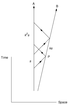
Figure 1: The $k$-calculus.

Denoting changes by $\Delta T$, $\Delta X$, etc, we have

$$\Delta T=\textstyle{1\over 2}(\Delta S_{\mathrm{r}}+\Delta S_{\mathrm{e}})=\textstyle{1\over 2}(k^{2}+1)s$$

(1)

$$\Delta X=\textstyle{1\over 2}(\Delta S_{\mathrm{r}}-\Delta S_{\mathrm{e}})=\textstyle{1\over 2}(k^{2}-1)s$$

giving the velocity

$$v=\Delta X/\Delta T=(k^{2}-1)/(k^{2}+1)$$

or

$$k=\left({1+v\over 1-v}\right)^{1/2}.$$

Hence in this simple fashion the relativistic Doppler shift formula has been derived.

3 Discrete time

The space-time to be described here is constructed in exactly the above fashion, but assumes that proper-time intervals are discrete rather than continuous. Thus for example the interval between A’s emission of the two flashes in the above experiment must be measured by a positive integer $n_{\mathrm{e}}$ rather than by a continuous real number $s$. Similarly the interval between A’s reception of the two echoes is measured by another positive integer $n_{\mathrm{r}}$. We now define the $k$-factor characterising B’s motion by

$$k^{2}=n_{\mathrm{r}}/n_{\mathrm{e}}$$

(2)

and B’s velocity relative to A by

$$v=(n_{\mathrm{r}}-n_{\mathrm{e}})/(n_{\mathrm{r}}+n_{\mathrm{e}}).$$

(3)

At this stage, the model runs into severe difficulties as a model of the real world, as equations (2) and (3) restrict $k^{2}$ and $v$ to rational values. Moreover, the result of a determination of B’s velocity will depend upon which pulse emission interval A decides to use. For example, A might use a large value, say $n_{\mathrm{e}}=10^{6}$, in one determination, and observe say $n_{\mathrm{r}}=10^{6}+2$, giving $v=10^{-6}$, i.e. $300$ m s^-1. In a second determination A might choose a small interval, say the extreme case $n_{\mathrm{e}}=1$; the smallest non-zero velocity in this case is given by $n_{\mathrm{e}}=2$, and is $v=1/3$, i.e. $10^{8}$ m s^-1.

These problems are similar to those encountered in Schild’s model; they disappear if we drop the assumption that $n_{\mathrm{r}}$ is precisely determined by $n_{\mathrm{e}}$. For example, observer A might conduct a series of experiments to determine the velocity of a given particle B. In each experiment, A allows the same integer interval $n_{\mathrm{e}}$ between sending out the two light flashes. In the model advocated here, the values of $n_{\mathrm{r}}$ observed in such a series need not be identical; this is taken as one of the axioms of the model. Instead all values of $n_{\mathrm{r}}$ can be observed, but do so with a frequency distribution which gives the correct mean value for the ratio in equation (2). In the above particular example with $n_{\mathrm{e}}=1$, the value $n_{\mathrm{r}}=1$ would be observed in almost all experiments, and $n_{\mathrm{e}}=2$ in only about three experiments per million conducted.

Thus we have a model of space-time with an inbuilt indeterminacy. All that is needed to complete the picture is a specification of the frequency distribution of the observed number $n_{\mathrm{r}}$. The natural choice is the Poisson distribution, which finds a number of applications in physics. For example, in a gas the number of atomic collisions experienced by any one atom in unit time is a random integer distributed in this fashion; if $P_{n_{\mathrm{c}}}$is the probability of making $n_{\mathrm{c}}$ such collisions, we have

$$P_{n_{\mathrm{c}}}=n_{\mathrm{m}}^{n_{\mathrm{c}}}\rme^{-n_{\mathrm{m}}}/n_{\mathrm{c}}!$$

where $n_{\mathrm{m}}$ is the mean number of collisions per unit time. I shall assume such a distribution for $n_{\mathrm{r}}$. In the series of experiments described above, we require

$$P_{n_{\mathrm{e}},n_{\mathrm{r}}}=(k^{2}n_{\mathrm{e}})^{n_{\mathrm{r}}}\rme^{-k^{2}n_{\mathrm{e}}}/n_{\mathrm{r}}!$$

(4)

This is the probability that if A chooses a pulse emission interval $n_{\mathrm{e}}$, he will observe an echo reception interval $n_{\mathrm{r}}$. The factor $k^{2}$ characterising B’s motion relative to A is now the mean value of the ratio $n_{\mathrm{r}}/n_{\mathrm{e}}$, rather than the value resulting from a particular observation; $k^{2}$ is thus not restricted to rational values. Similarly, the mean of the velocity defined by equation (3) can have any value between $-1$ and $+1$. The standard deviation of $n_{\mathrm{r}}$ is exactly $kn_{\mathrm{e}}^{1/2}$, so that $n_{\mathrm{r}}/n_{\mathrm{e}}\rightarrow k^{2}$ as $n_{\mathrm{e}}\rightarrow\infty$; hence we recover the classical picture over sufficiently long intervals, when the indeterminacy is of negligible proportions.

4 The nature of time

It may be that the above analogy with the kinetic theory of gases is more than just an analogy. I have a picture of space-time as in some sense comprising a sea of particles which I shall call chronons. Other particles float in this sea and sense a continual chronon bombardment; this sensation is called time. I have found this physical picture a great conceptual aid, but it is not essential to the model, the essence of which is contained in the following purely mathematical postulates:

(i) Discreteness. Proper-time intervals are discrete and the structure of space- time is given by the radar map.

(ii) A correspondence principle. The integers, measuring any two time intervals which classically are causally related in a linear manner, are randomly related in such a way that specifying the one only fixes the mean of the other, this mean to coincide with the classical value.

(iii) The distribution. The probability function specifying the random behaviour is the Poisson distribution.

In what follows, I shall frequently use the expression ‘counting chronons’; it can be interpreted as meaning just the registering of discrete time elements; however, it may have a more literal meaning.

5 Lorentz invariance

The postulates of this space-time model do not assign a special position to any particular class of observers, so that the model must basically be Lorentz invariant. However, the indeterminacy will mask the invariance in any one observation. It is instructive to examine the $k$-calculus derivation (Bondi 1965) of the Lorentz transformation in the light of the ideas expounded above.  Observers A and B in Figure 2 move with relative

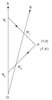
Figure 2: The Lorentz Transformation.

motion characterised by a factor $k$, and agree to start their chronon counters as they pass each other at event O. After counting $N_{\mathrm{e}}$ chronons A emits a light pulse to illuminate event P, and receives the echo after counting $N_{\mathrm{r}}$ chronons. Observer B similarly illuminates event P, the corresponding chronon counts being $N_{\mathrm{e}}^{\prime}$ and $N_{\mathrm{r}}^{\prime}$. A and B respectively assign (half-integral) coordinates $(T,X)$ and $(T^{\prime},X^{\prime})$ to this event, defined by

$$T=\textstyle{1\over 2}(N_{\mathrm{r}}+N_{\mathrm{e}})~{}~{}~{}~{}~{}~{}X=\textstyle{1\over 2}(N_{\mathrm{r}}-N_{\mathrm{e}})$$

$$T^{\prime}=\textstyle{1\over 2}(N_{\mathrm{r}}^{\prime}+N_{\mathrm{e}}^{\prime})~{}~{}~{}~{}~{}~{}X^{\prime}=\textstyle{1\over 2}(N_{\mathrm{r}}^{\prime}-N_{\mathrm{e}}^{\prime}).$$

Writing

$$N_{\mathrm{e}}^{\prime}/N_{\mathrm{e}}=k_{1}~{}~{}~{}~{}~{}~{}N_{\mathrm{r}}/N_{\mathrm{r}}^{\prime}=k_{2}$$

the equations

$$T^{\prime}=\textstyle{1\over 2}(k_{1}+1/k_{2})T-\textstyle{1\over 2}(k_{1}-1/k_{2})X$$

(5)

$$X^{\prime}=\textstyle{1\over 2}(k_{1}+1/k_{2})X-\textstyle{1\over 2}(k_{1}-1/k_{2})T$$

(6)

and

$$T^{\prime 2}-X^{\prime 2}=(k_{1}/k_{2})(T^{2}-X^{2})$$

are easily derived. Classically we would have

$$k_{1}=k_{2}=k=\left({1+v\over 1-v}\right)^{1/2}$$

when equations (5) and (6) are just the Lorentz transformation. In general we have $k_{1}\not=k_{2}$, so that these equations do not coincide with a Lorentz transformation. However,the correspondence principle ensures that the mean values of $k_{1}$ and $k_{2}$, taken over many similar observations, are equal to $k$, so that in this sense Lorentz invariance is maintained. Of course in the case of the macroscopic intervals $k_{1}$ and $k_{2}$ are so nearly equal that the lack of invariance would not be noticed.

6 Uncertainty

Modern classical and quantum physics are troubled by infinities in a number of areas; the possibility that these divergences might disappear if a difierent space-time model were to be adopted, with the equations of classical and quantum physics suitably rewritten, has been one of the motivations behind the search for such alternatives. Given such a model, the appropriate reformulation of the laws might not be unambiguously indicated. In this context, the present model offers almost an embarrassment of riches, as any reformulation of classical physics necessarily leads to laws which reflect the indeterminacy in the model. A reformulation of quantum theory, with its inherent uncertainty, within the present framework, might lead to too much indeterminacy. A tempting point of view is that this model plus classical physics might be an alternative to classical space-time plus quantum theory. An intermediate viewpoint is that this model might make the ‘second quantisation’ programme unnecessary. The present model is hardly sufficiently well developed to permit a general reformulation of the kind discussed above. However, we can examine the most elementary classical dynamical concept, namely the one-dimensional motion of a free particle. Consider first a non-relativistic case: an observer A and an elementary particle B of mass $m$ at rest relative to A, in the sense that $k=1$ in the distribution (4). A carries out a radar determination of B’s velocity using a flash emission interval $n_{\mathrm{e}}$; in general A will observe an echo reception interval $n_{\mathrm{r}}\not=n_{\mathrm{e}}$, so that according to equation (3) B does not appear to be at rest at all; over a series of such experiments, B has a mean square velocity $\langle v^{2}\rangle$ given by

$$\langle v^{2}\rangle=\langle\left({n_{\mathrm{r}}-n_{\mathrm{e}}\over n_{\mathrm{r}}+n_{\mathrm{e}}}\right)^{2}\rangle\sim{{\langle(n_{\mathrm{r}}-n_{\mathrm{e}})^{2}\rangle}\over 4n_{\mathrm{e}}^{2}}.$$

Distribution (4) with $k=1$ gives $\langle(n_{\mathrm{r}}-n_{\mathrm{e}})^{2}\rangle=n_{\mathrm{e}}$, giving

$$\langle v^{2}\rangle=1/4n_{\mathrm{e}}$$

which constitutes an estimate of B’s energy. As the true energy of B is zero, this estimate is in error by an amount

$$\Delta E=\textstyle{1\over 2}m\langle v^{2}\rangle\sim m/8n_{\mathrm{e}}.$$

This estimate refers to B’s motion during a time interval for the observer of extent $\Delta t=n_{\mathrm{r}}\sim n_{\mathrm{e}}$. The product $\Delta E\Delta t$ is thus given by

$$\Delta E\Delta t\sim m/8.$$

(7)

If $n_{\mathrm{s}}$ is the number of chronon counts corresponding to one second, then $\Delta t$ must be divided by $n_{\mathrm{s}}$ to convert it into seconds. In conventional units, equation (7) thus becomes

$$\Delta E\Delta t\sim mc^{2}/8n_{\mathrm{s}}.$$

(8)

Apart from an ambiguity relating to the mass $m$, this is precisely Heisenberg’s uncertainty relation, if we identify Plank’s constant $\hbar$ as

$$\hbar=mc^{2}/8n_{\mathrm{s}}$$

or

$$n_{\mathrm{s}}=mc^{2}/8\hbar=2\pi c/8\lambda_{\mathrm{c}}$$

(9)

where $\lambda_{\mathrm{c}}$ is the Compton wavelengh of the particle B. For an electron the particle wavelength is $\lambda_{\mathrm{c}}=2.42\times 10^{-10}$ cm; equation (9 ) then gives a discrete time element of about $10^{-20}$ s. The corresponding length element is just $c/n_{\mathrm{s}}\sim 8\lambda_{\mathrm{c}}/2\pi$, so that the space-time model under discussion certainly fits in with the notion of continuity breakdown at the elementary particle level.

To generalise equation (7) to the case of a particle actually moving, in the sense that $k\not=1$, we note that the total energy $E$ is given by

$$E=\textstyle{1\over 2}m[(n_{\mathrm{r}}/n_{\mathrm{e}})^{1/2}+(n_{\mathrm{e}}/n_{\mathrm{r}})^{1/2}].$$

We write

$$n_{\mathrm{r}}=k^{2}n_{\mathrm{e}}+n$$

where $n$ is the deviation of $n_{\mathrm{r}}$ from its mean value $k^{2}n_{\mathrm{e}}$, and is of order $kn_{\mathrm{e}}^{1/2}$. Expanding $E$ in powers of $n$, we find

$$E=E_{0}+\textstyle{1\over 2}p_{0}(n/k^{2}n_{\mathrm{e}})+\textstyle{1\over 8}(m/k-p_{0})(n/k^{2}n_{\mathrm{e}})^{2}$$

$$~{}~{}~{}~{}~{}~{}~{}~{}~{}~{}~{}~{}~{}~{}~{}~{}~{}~{}~{}~{}~{}~{}~{}~{}~{}~{}~{}~{}~{}~{}~{}~{}~{}-\textstyle{1\over 16}(2m/k-p_{0})(n/k^{2}n_{\mathrm{e}})^{3}+...$$

(10)

where

$$E_{0}=\textstyle{1\over 2}(k+1/k)m~{}~{}~{}~{}~{}~{}\hbox{and}~{}~{}~{}~{}~{}~{}p_{0}=\textstyle{1\over 2}(k-1/k)m$$

are the classical energy and momentum of the particle, i.e. as revealed over long observation intervals. On averaging over $n$, equation (10) gives

$$\langle E\rangle=E_{0}+\textstyle{1\over 8}(m/k-p_{0})/k^{2}n_{\mathrm{e}}+...$$

(11)

and

$$\Delta E^{2}=\langle E^{2}\rangle-{\langle E\rangle}^{2}$$

(12)

$$~{}~{}~{}~{}~{}~{}=\left(\textstyle{1\over 2}p_{0}\right)^{2}/(k^{2}n_{\mathrm{e}})+[\textstyle{1\over 32}(m/k-p_{0})^{2}-\textstyle{3\over 16}p_{0}(2m/k-p_{0})]/(k^{2}n_{\mathrm{e}})^{2}+...$$

The observation interval is $\Delta t=n_{\mathrm{r}}/n_{\mathrm{s}}\sim k^{2}n_{\mathrm{e}}/n_{\mathrm{s}}$; equations (9) and (12) together give

$$\Delta E\Delta t$$

(13)

$$=[\left(4p_{0}/m\right)^{2}k^{2}n_{\mathrm{e}}+2(1/k-p_{0}/m)^{2}-12(p_{0}/m)(2/k-p_{0}/m)+...]^{1/2}\hbar$$

which is the full uncertainty relationship, accurate up to moderately relativistic momenta. Equation (13) implies

$$\Delta E\Delta t~{}^{>}_{\sim}~{}[2(1/k-p_{0}/m)^{2}-12(p_{0}/m)(2/k-p_{0}/m)]^{1/2}\hbar.$$

The approximate equality holds if

$$k^{2}n_{\mathrm{e}}<\textstyle{1\over 8}[(1/k)(m/p_{0})-1]^{2}-\textstyle{3\over 4}[(2/k)(m/p_{0})-1]\sim\textstyle{1\over 8}c^{2}/v^{2}$$

which is equivalent to

$$\Delta t<{1\over 2\pi}{c^{2}\over v^{2}}{\lambda_{c}\over c}.$$

A simple expression showing the deviation of B’s motion from its classical path can be derived. We consider the expression (4) for $P_{n_{\mathrm{e}},n_{\mathrm{r}}}$ and use Stirling’s approximation:

$$n_{\mathrm{r}}!\sim(2\pi n_{\mathrm{r}})^{1/2}n_{\mathrm{r}}^{n_{\mathrm{r}}}\rme^{-n_{\mathrm{r}}}.$$

For moderately large values of $n_{\mathrm{r}}$, equation (4) becomes

$$P_{n_{\mathrm{e}},n_{\mathrm{r}}}\sim(2\pi n_{\mathrm{r}})^{-1/2}\hbox{exp}[-\textstyle{1\over 2}(n_{\mathrm{r}}-k^{2}n_{\mathrm{e}})^{2}/k^{2}n_{\mathrm{e}}].$$

(14)

We interpret this as follows: $n_{\mathrm{e}}$ is the interval between two light flashes emitted by A, to make two determinations of B’s position. For simplicity I shall assume that the first is emitted as A and B pass (and hence returns immediately), and that A chooses this event as his space-time origin. If the second position so determined has coordinates $(t,x)$, we have

$$n_{\mathrm{e}}=t-x$$

$$n_{\mathrm{r}}=t+x$$

and

$$n_{\mathrm{r}}-k^{2}n_{\mathrm{e}}=(k^{2}+1)(x-v_{0}t)$$

where $v_{0}=(k^{2}-1)/(k^{2}+1)$ is the classical velocity of B. Equation (14) thus becomes

$$P_{t,x}=[2\pi(t+x))]^{-1/2}\hbox{exp}[-\textstyle{1\over 2}(k^{2}+1)^{2}(x-v_{0}t)^{2}/k^{2}(t-x)].$$

This is the probability that after time $t$ the particle B is observed at position $x$; we see that this position has a Gaussian spread about the classical path $x=v_{0}t$.

7 Recapitulation

Classical physics deals with systems having a continuous spectrum of states, and allows a system to be precisely located within this spectrum. In general quantum physics permits only a discrete spectrum, but allows the state of a system to spread over this spectrum according to a probability function. In this way classical and quantum physics can ‘correspond’ in the appropriate limit. A similar contrast can be drawn between the classical picture of time and the one presented here; in this sense the theory discussed here is a quantum theory of time.

The results presented in §6 relating to the motion of non-interacting particles are remarkably similar to quantum mechanical ones; it seems that any attempt to reformulate physics within this framework might start with classical physics, and might reproduce quantum theory, with hopefully some experimentally observable differences. The one unsatisfactory feature of the derivation of the uncertainty principle is the ambiguity relating to the mass $m$ of particle B. Equation (8) suggests a resolution of this ambiguity, which however involves taking seriously the chronon impact picture of time. If we regard the discrete elements of time as actual intervals between chronon impacts, we must specify a chronon register to be used in for example radar observations of particle motion. Clearly a macroscopic clock will experience many more such impacts in a given interval than say an electron, in direct proportion to the number of particles in the clock, i.e. its rest mass. If we adopt the notion that when observing the motion of say electrons, then electrons are to be regarded as chronon impact registers, the resolution suggested by equation (8) is that the number of such impacts in a given interval is proportional to the rest mass of the particle in question, i.e. that the rest mass is proportional to the chronon collision cross section. The ratio $m/n_{\mathrm{s}}$ is thus constant, and equation (8) is now an unambiguous statement. If this idea is correct, it implies that space-time continuity breaks down at different levels for difierent species of elementary particle. An immediate consequence of this idea is that zero rest mass particles do not register chronons at all, which is quite acceptable as such particles follow null paths.

There is of course a danger that the chronon gas would define an absolute rest frame, in the way that a classical gas of atoms or photons would. However, there is a fundamental difference here, which might prevent this. A particle moving slowly relative to the rest frame defined by say a classical relativistic gas would experience fewer atomic collisions per second than one at rest in this frame; by definition, the number of chronon impacts per unit time is the same for all particles of one species, whatever their relative motion. In any case, the chronon gas is not to be taken as filling space in the classical fashion, but as ‘being’ space-time in some sense, along the lines of Penrose’s idea of a ‘no space-time’ model of space-time (Penrose 1967).

In conclusion, we note that this discussion has been restricted to one spatial dimension, and to the one-dimensional motion of non-interacting particles. Clearly generalisations are required to produce a fully workable model. A generalisation to three spatial dimensions would involve a discussion of angles and directions, which might enable a theory of angular momentum to be developed. Gravitation, within the framework of classical general relativity, would probably be the easiest interaction to consider in this context, as there has been extensive work (Ehlers et al 1972; Castagnino 1971) on the construction of curved space-time structure using light rays and free particles.

References

Bondi H 1965 Brandeis Lectures, 1964 vol. 1 (Englewood Cliffs, NJ: Prentice-Hall)
 pp 386-399
Castagnino M 1971 J. Math. Phys. 12 2203
Chew G F 1963 Sci. Prog. 5l October 529
Ehlers J, Pirani F A E and Schild A 1972 General Relativity: Volume Dedicated to
 J L Synge (London: Oxford University Press)
Penrose R 1967 Adams prize Essay: An analysis of the structure of space-time
 (unpublished)
Schild A 1948 Phys. Rev. 73 414