SUPERNOVAE AND AGN DRIVEN GALACTIC OUTFLOWS

Abstract

We present analytical solutions for winds from galaxies with NFW dark matter halo. We consider winds driven by energy and mass injection from multiple supernovae (SNe), as well as momentum injection due to radiation from a central black hole. We find that the wind dynamics depends on three velocity scales: (a) $v_{\star}\sim(\dot{E}/2\dot{M})^{1/2}$ describes the effect of starburst activity, with $\dot{E},\dot{M}$ as energy and mass injection rate in a central region of radius $R$; (b) $v_{\bullet}\sim(GM_{\bullet}/2R)^{1/2}$ for the effect of a central black hole of mass $M_{\bullet}$ on gas at distance $R$ and (c) $v_{s}=(GM_{h}/2\mathcal{C}r_{s})^{1/2}$ which is closely related to the circular speed ($v_{c}$) for NFW halo, with $r_{s}$ as the halo scale radius and $\mathcal{C}$ is a function of halo concentration parameter. Our generalized formalism, in which we treat both energy and momentum injection from starbursts and radiation from central active galactic nucleus (AGN), allows us to estimate the wind terminal speed to be $(4v_{\star}^{2}+6(\Gamma-1)v_{\bullet}^{2}-4v_{s}^{2})^{1/2}$, where $\Gamma$ is the ratio of force due to radiation pressure to gravity of the central black hole. Our dynamical model also predicts the following: (a) winds from quiescent star forming galaxies cannot escape from $10^{11.5}\leq M_{h}\leq 10^{12.5}$ M_☉ galaxies, (b) circumgalactic gas at large distances from galaxies should be present for galaxies in this mass range, (c) for an escaping wind, the wind speed in low to intermediate mass galaxies is $\sim 400\hbox{--}1000$ km/s, consistent with observed X-ray temperatures; (d) winds from massive galaxies with AGN at Eddington limit have speeds $\gtrsim 1000$ km/s. We also find that the ratio $[2v_{\star}^{2}-(1-\Gamma)v_{\bullet}^{2}]/v_{c}^{2}$ dictates the amount of gas lost through winds. Used in conjunction with an appropriate relation between $M_{\bullet}$ and $M_{h}$, and an appropriate opacity of dust grains in infrared (K band), this ratio has the attractive property of being minimum at a certain halo mass scale ($M_{h}\sim 10^{12\hbox{--}12.5}$ M_☉) that signifies the cross-over of AGN domination in outflow properties from starburst activity at lower masses. We find that stellar mass for massive galaxies scales as $M_{\star}\propto M_{h}^{0.26}$, and for low mass galaxies, $M_{\star}\propto M_{h}^{5/3}$.

1. Introduction

In the standard scenario of galaxy formation the baryonic matter falls inside the potential wells created by dark matter halos. This in-falling material cools and forms stars. This picture is met with problems as the galaxy stellar mass function does not follow the halo mass function. Both low and high mass halos have significantly lower than predicted value of stellar masses (Somerville et al. 2008; Moster et al. 2010; Behroozi et al. 2010). To reconcile with these problems it has been proposed that the SNe and starbursts provide thermal energy injection and cause large amount of mass to flow out of the galaxy as galactic superwinds (Dekel & Silk 1986; Larson 1974; Oppenheimer & Davé 2006). The star formation is suppressed as the galaxies lose a significant portion of their baryons due to this negative feedback. Although this picture can provide explanation for the low ratios of $M_{\star}/M_{h}$ for the low mass halos, but for the high mass halos, gravity becomes strong and the SNe are not sufficient to drive the gas out. In order to resolve the discrepancy at high mass end, it has been argued that the AGN outflows may sweep away the baryons and suppress the star formation in high mass galaxies (Silk & Rees 1998; Wyithe & Loeb 2003; Di Matteo et al. 2005; Springel et al. 2005; Croton et al. 2006; Bower et al. 2006). These two feedback processes, when considered together, are believed to explain the shape of galaxy stellar mass function at both low and high mass end (Binney 2004; Cattaneo et al. 2006; Puchwein & Springel 2012).

Apart from their cosmological importance as a feedback process, galactic winds have been a topic of research as a gas dynamical problem in galactic physics. Speculations on the possibility that galaxies can harbour large scale winds followed the models of solar wind developed by Parker (1965). Burke (1968) proposed a model of trans-sonic winds from the galaxy with heat and mass addition from SNe. It was further proposed that galactic winds may cause ellipticals to lose all of their gas (Johnson & Axford 1971; Mathews & Baker 1971). The review by Holzer & Axford (1970) gives an elaborate account of the theoretical aspects of solar and galactic winds. Chevalier & Clegg (1985) showed that energy injection at the center can drive a fast super-wind from the dwarf star-burst galaxy M82. In this work the gravity of the galaxy was not considered and the obtained solutions were trans-sonic with a heat injection up to the sonic point. Wang (1995) modeled the wind from a power law gravitational potential and showed that wind may escape the galaxy or settle in a galactic corona depending on the mass of the galaxy and the effect of radiative cooling. Silich et al. (2011) studied the effects of cooling on winds from individual star clusters with exponential stellar density distribution. Winds driven by cosmic rays have also been studied in the literature (Ipavich 1975; Breitschwerdt et al. 1991; Samui et al. 2008; Uhlig et al. 2012).

Observations show that the winds do not consist of a homogeneous medium. The hot gas emitting X-rays and the cold/warm gas visible in emmision and absorption lines (Strickland et al. 2004; Bouché et al. 2012; Kornei et al. 2012), coexist in the galactic winds (Heckman et al. 2000; Veilleux et al. 2005). Hot phase appears as a smooth flow of tenuous gas while the colder phase is clumpy in nature. It is usually believed that cold neutral clouds form as a result of thermal instabilities in the hot flow and they are entrained with the parent flow because of its ram pressure (Heckman et al. 1993). Hydrodynamical simulations with radiative cooling also supported this scenario (Suchkov et al. 1994; Strickland & Stevens 2000; Cooper et al. 2008). However, recent observations show that the velocity of neutral clouds does not correlate with the velocity of hot flow and rather it correlates with the circular speed of the host galaxy (Martin 2005; Rupke et al. 2005b). If one considers the momentum driven winds where the radiation from the galaxy acts on the dust grains, then these observations can be explained (Murray et al. 2005; Sharma et al. 2011; Chattopadhyay et al. 2012; Nath & Silk 2009). However the radiation may not be sufficient in fainter low mass galaxies and ram pressure is still required to explain the cold winds in these galaxies (Sharma & Nath 2012; Murray et al. 2011; Hopkins et al. 2012). On the other hand in high mass ULIRGs, radiation from AGN may be an alternate mechanism for driving outflows apart from SNe and stellar radiation.

In spite of the general consensus about the AGN driving in quasar outflows, observationally it has been hard to establish that outflows in galaxies are also powered by AGN (Rupke et al. 2005a; Westmoquette et al. 2012). However, recent observations do show compelling evidence for the AGN driving in galactic outflows (Sturm et al. 2011; Rupke & Veilleux 2011; Alexander et al. 2010; Morganti et al. 2007; Dunn et al. 2010; Feruglio et al. 2010; Fu & Stockton 2009; Villar-Martín et al. 2011). From the theoretical point of view, considerable amount of work has been carried out in modeling radiation driven outflows in the immediate vicinity of the AGN (Murray et al. 1995; Proga et al. 2000; Kurosawa & Proga 2009; Risaliti & Elvis 2010). However, the effects of radiation from accreting black holes has not been discussed for driving galaxy scale outflows. Murray et al. (2005) proposed the existence of a critical luminosity for the AGN (or the galaxy) necessary for the blow-out of all the available gas. The value of this critical luminosity depends on the dust scattering opacity at UV. Everett & Murray (2007) studied Parker wind from AGN occurring at scales of $\sim 100$ pc. Debuhr et al. (2012) carried out simulations showing that the initial momentum injection and the fast outflow in the vicinity of hole may shock the surrounding ISM and can result in a galaxy scale outflow. Whether the outflows due to the AGN are energy conserving or momentum conserving has been a topic of debate as well. Silk & Nusser (2010) argued that the energy driven outflows are not possible in the galactic bulges. King et al. (2011) proposed that AGN outflows are momentum driven at small scales and energy driven on larger scales. Faucher-Giguère & Quataert (2012) showed that the cooling in the region, shocked by AGN radiation pressure, may not be effective and the outflows can be energy conserving. McQuillin & McLaughlin (2012) studied the large scale motion of momentum-conserving supershells from a dark matter halo. Novak et al. (2012) carried out a radiation transfer calculation assessing the efficiency of various components of AGN spectrum in driving outflows. This work showed that most of the UV flux is quickly absorbed and re-radiated in IR. The IR radiation can drive a dusty outflow and may result in mass loss much higher than the line driving mechanisms, on the scales connecting the AGN and host galaxy as shown by radiation hydrodynamic simulations (Dorodnitsyn et al. 2011) .

It is evident from the studies on starburst and AGN driven outflows that these processes play an important role in the formation and evolution of galaxies. In galaxy formation models, these two processes are generally invoked using simple recipes through feedback factors. However, in theoretical models of winds they have been treated separately for the low mass and high mass galaxies. There is a lack of models that develop a complete hydrodynamic theory of winds which can envisage both these feedback processes. In the present paper we address this problem analytically and bring in both these wind driving agents together and using the analytical results from our calculation we also attempt an explanation for the galaxy stellar to halo mass relation.

We start with the derivation of a general wind equation in §2, which accounts for any possible mass, energy and momentum injection. We then present a brief derivation of SNe driven wind model of CC85 and extend this model to the case including a dark matter halo in §3. Afterwards in §5 we introduce the momentum injection from the AGN and derive a general analytic solution for the galactic wind, which has inputs from SNe injection, NFW gravity and the central black hole. This solution leads us to important results like the terminal velocity of winds, condition for escaping winds and the dependence of wind properties on the halo mass and the black hole mass. In §5.2 we show the velocity, density and temperature of the outflow as a function of the distance from the center. Interestingly a class of our solutions can explain the gas reservoirs in the the galactic halos seen in observations (Tumlinson et al. 2011) and simulations (van de Voort & Schaye 2012; Stinson et al. 2012). In §5.3 we study the cosmological implications of our results. We derive the scaling relation between stellar ($M_{\star}$) and halo mass ($M_{h}$) using simple recipes and inputs from our models. We compare our analytically derived stellar to halo mass ratio (SHMR) with the observations and results of abundance matching. We discuss our results in §6.

2. Basic equations

We consider steady spherically symmetric winds driven by mass and energy/momentum injection from processes that are confined in a central region of radius $R$. Consider a heating rate $\dot{E}$ and mass injection rate $\dot{M}$ in this region, which has a size of a few hundred parsecs (see below) then the basic fluid equations can be written as,

$${1\over r^{2}}\frac{d}{dr}(\rho vr^{2})=\dot{m}={\dot{M}\over V}$$ (1)

$$v\frac{dv}{dr}=-{1\over\rho}{dp\over dr}-{d\Phi\over dr}+f(r)-{\dot{m}v\over\rho}$$ (2)

$${1\over r^{2}}{d\over dr}\left[\rho vr^{2}\left(\frac{v^{2}}{2}+{c_{s}^{2}\over\gamma-1}\right)\right]+\rho v\left(\frac{d\Phi(r)}{dr}-f(r)\right)=q={\dot{E}\over V}$$ (3)

Here $V$ is the volume of the central region in which the energy injection and the mass injection is occurring. $\Phi(r)$ represents the gravitational potential and $f(r)$ is the momentum injection force per unit mass. $c_{s}$ is the Laplacian sound speed. In this work we will be considering the momentum injection from the AGN in optically thin limit hence the $f(r)$ has an inverse square dependence on $r$. The above written system of equations do not have a critical point if the heating and mass injection is zero. However, for a finite energy and mass injection there is a critical point. For an extended energy and mass distribution the critical point can be determined numerically as done for super star-cluster winds in Silich et al. (2011). To extract maximum information analytically we have considered the energy and mass injection to be confined in a region of radius $r=R$ following Chevalier & Clegg (1985, hereafter CC85). Therefore in the present case the critical point is situated right at the boundary of central injection region.

In this work we do not consider the radiative cooling, as it is generally believed that the energy loss via radiation over the entire wind is small and less dominant than the adiabatic loss (Grimes et al. 2009), hence the cooling does not affect the dynamics of the flow. However it may still be important for the thermodynamics of the flow (see appendix D) and may result in the precipitation of the wind which can not be dealt with the steady stable flow solutions. The dynamics and survival of clouds formed by thermal instability in the galactic wind is also an important issue and it has been studied elsewhere in the category of cold winds (Murray et al. 2011; Sharma & Nath 2012; Marcolini et al. 2005; Cooper et al. 2009). Therefore, we distinguish our model from that of the clumpy winds and in the present work we study analytically the large scale dynamics of homogeneous steady outflow from a NFW dark matter halo and its cosmological implications.

By introducing the mach number $\mathcal{M}=v/c_{s}$, the above equations can be transformed to the following ordinary differential equation (see Appendix A for a complete derivation).

$$\frac{\mathcal{M}^{2}-1}{\mathcal{M}^{2}(\mathcal{M}^{2}(\gamma-1)+2)}\frac{d\mathcal{M}^{2}}{dr}={2\over r}-(1+\gamma\mathcal{M}^{2}){\dot{m}\over\rho v}-\frac{\dot{m}(1+\gamma\mathcal{M}^{2})}{2\rho v}\left(\frac{\dot{E}/\dot{M}}{\epsilon(r)}-1\right)+\frac{(\gamma+1)\left(f(r)-\frac{d\Phi(r)}{dr}\right)}{2(\gamma-1)\epsilon(r)}$$ (4)

where $\dot{m}=\dot{M}/V$ and $\epsilon(r)=\frac{v^{2}}{2}+\frac{c_{s}^{2}}{\gamma-1}$. We will use $\gamma=5/3$. As mentioned above, the terms $\dot{E}$ and $\dot{M}$ represent the energy and mass injection in a central region of size $r=R$, beyond which they become zero. We use $R=200$ pc for the present work.

2.1. Zero gravity case: Chevalier & Clegg’s solution

In this section we briefly reproduce the CC85 solution, therefore this subsection also serves as a consistency check for equation 4. In the CC85 solution gravitational force of the galaxy is not considered as the wind speeds were of the order of thousand km s^-1which is an order of magnitude larger than the circular speed of starburst galaxy M82. There is no external driving force ($f(r)=0$). Hence the main driving force is the energy injection from SNe in a central $200$ pc region. The size of the central region also marks the boundary where the energy injection and the subsonic part ends. The wind equation then can be solved analytically for subsonic ($\mathcal{M}<1$) and supersonic ($\mathcal{M}>1$) part of the wind.

In order to derive the subsonic part of the solution, we can use $\dot{m}={3\rho v/r}$ which results from the integration of continuity equation. Therefore equation 4 becomes

$$\frac{\mathcal{M}^{2}-1}{\mathcal{M}^{2}(\mathcal{M}^{2}(\gamma-1)+2)}\frac{d\mathcal{M}^{2}}{dr}={2\over r}-{3(1+\gamma\mathcal{M}^{2})\over r}-\frac{3(1+\gamma\mathcal{M}^{2})}{2\ r}\left(\frac{\dot{E}/\dot{M}}{\epsilon(r)}-1\right)$$ (5)

Direct integration of energy equation 3 by retaining the energy and mass injection and neglecting the gravity and external driving results in, $\epsilon(r)={\dot{E}/\dot{M}}=2v_{\star}^{2}\,,$ where we have defined a velocity parameter, $v_{\star}=\sqrt{\dot{E}/2\dot{M}}$ . It can be shown that at the critical point, $v_{\rm crit}=v(R)=c_{s}(R)=v_{\star}$. Substituting this $\epsilon(r)$ in equation 5, we get,

$$\frac{\mathcal{M}^{2}-1}{\mathcal{M}^{2}[(\gamma-1)\mathcal{M}^{2}+2]}\frac{d\mathcal{M}^{2}}{dr}=\frac{-1-3\gamma\mathcal{M}^{2}}{r}$$ (6)

This can be integrated to get the following solution,

$$\delta_{<}(\mathcal{M})=\left(\frac{3\gamma+1/\mathcal{M}^{2}}{3\gamma+1}\right)^{-\frac{3\gamma+1}{5\gamma+1}}\left(\frac{\gamma-1+2/\mathcal{M}^{2}}{\gamma+1}\right)^{\frac{\gamma+1}{2(5\gamma+1)}}=\frac{r}{R}\ ;\quad\quad r<R$$ (7)

Following similar steps and additionally dropping the injection terms, we can evaluate supersonic part of the solution. Analytically it implies setting $\Phi=f=\dot{M}=\dot{E}=0$ in the wind equation 4. Therefore, we are left with the following differential equation,

$$\frac{\mathcal{M}^{2}-1}{\mathcal{M}^{2}[(\gamma-1)\mathcal{M}^{2}+2]}\frac{d\mathcal{M}^{2}}{dr}=\frac{2}{r}$$ (8)

This can be integrated to get the following solution for the supersonic part of the wind,

$$\delta_{>}(\mathcal{M})=\mathcal{M}^{{2\over\gamma-1}}\left(\frac{\gamma-1+2/\mathcal{M}^{2}}{\gamma+1}\right)^{\frac{\gamma+1}{2(\gamma-1)}}=\left(\frac{r}{R}\right)^{2}\ ;\quad\quad r>R$$ (9)

These expressions were arrived at by CC85. We shall use these definitions of $\delta_{<}(\mathcal{M})$ and $\delta_{>}(\mathcal{M})$ in the rest of the paper. The terminal velocity of the wind in this solution can be obtained easily from the energy equation which gives $\epsilon(r)=v^{2}/2+c_{s}^{2}/(\gamma-1)=2v_{\star}^{2}$. For $r\rightarrow\infty$, the sound speed can be neglected and we get $v_{\infty}=2v_{\star}=(2\dot{E}/\dot{M})^{1/2}$ . In the supersonic part of the wind for $\mathcal{M}>1$ the relation in equation 9 can be approximated by $\mathcal{M}^{3}\propto r^{2}$. Therefore, when the velocity attains its terminal value, then $c_{s}^{2}\propto T\propto r^{-4/3}$ and $\rho\propto r^{-2}$.

3. SN driven winds from NFW halo

In this section we study the effects of NFW dark matter halo on the wind velocity in detail. One can therefore consider the calculation in this section as an extension of the supersonic part of CC85 solution. We proceed first by fixing the dark matter halo parameters in the next subsection.

3.1. Dark matter halo properties

Here we discuss the properties of the NFW dark matter halo which will be used throughout the rest of the paper. We consider a Navarro Frank and White(NFW) dark matter halo with a density profile $\rho=\rho_{s}r_{s}^{3}/r(r+r_{s})^{2}$ (Navarro et al. 1996). For a dark matter halo of total mass $M_{h}$, which collapses at a redshift $z$, the virial radius is given by $r_{\rm vir}=[3M_{h}/(4\pi\Delta_{c}(z)\Omega_{m}^{z}\rho_{crit})]^{1/3}(1+z)^{-1}$ Where $\Delta_{c}$ is the critical over density which can be written as $\Delta_{c}(z)=18\pi^{2}-39d_{z}^{2}+82d_{z}$, with $d_{z}=\Omega_{m}^{z}-1$ and $\Omega_{m}^{z}=\frac{\Omega_{m}(1+z)^{3}}{\Omega_{m}(1+z)^{3}+\Omega_{\Lambda}+\Omega_{k}(1+z)^{2}}$ with parameters having their usual meaning (Bryan & Norman 1998; Bullock et al. 2001). We set $\Omega_{m}=0.258,\ \Omega_{\Lambda}=0.742,\ h=0.72$, according to the results from WMAP5 (Komatsu et al. 2009). Using these values, the virial radius can be written as

$$r_{\rm vir}=210\ \left({M_{h}\over 10^{12}\ {\rm M}_{\odot}}\right)^{1/3}\left[{\Omega_{m}\over\Omega_{m}^{z}}{\Delta_{c}(z)\over 18\pi^{2}}\right]^{-1/3}(1+z)^{-1}\ \ {\rm kpc}$$ (10)

The corresponding circular speed is, $v_{c}=\sqrt{GM_{h}/r_{\rm vir}}$. So it can be written as,

$$v_{c}=143\ \left({M_{h}\over 10^{12}\ {\rm M}_{\odot}}\right)^{1/3}\left[{\Omega_{m}\over\Omega_{m}^{z}}{\Delta_{c}(z)\over 18\pi^{2}}\right]^{1/6}(1+z)^{1/2}\ \ {\rm km\ s^{-1}}$$ (11)

The gravitational potential due to the NFW dark matter halo can be written as,

$$\Phi_{\rm NFW}=-{GM_{h}\over\ln(1+c)-c/(1+c)}\ {\ln(1+r/r_{s})\over r}=-2v_{s}^{2}\ {\ln(1+r/r_{s})\over r/r_{s}}$$ (12)

In this $v_{s}^{2}=GM_{h}/2\mathcal{C}r_{s}$ and $\mathcal{C}=\ln(1+c)-c/(1+c)$. Also $r_{s}=r_{\rm vir}/c$ is the NFW scale radius with $c$ as the halo concentration parameter which depends on both halo mass and the redshift of virialization. We use the fitting formula for $c$ given by Muñoz-Cuartas et al. (2011).

3.2. Effect of dark matter halo on winds

We study the effect of gravity in the supersonic part of the solution. In the subsonic part, the NFW gravity does not make a difference as shown in Appendix B. Therefore the subsonic part is same as in the previous section and we can assume that the energy injection propels the gas to a speed of $v_{\rm crit}=v_{\star}=(\dot{E}/2\dot{M})^{1/2}$ at the critical point. To study the supersonic solution beyond the critical point ($r>R$) , we set $\dot{E}$ and $\dot{m}$ equal to zero, and use the NFW potential in equation 4, which results in the following equation for the supersonic part,

$$\frac{\mathcal{M}^{2}-1}{\mathcal{M}^{2}[(\gamma-1)\mathcal{M}^{2}+2]}\frac{d\mathcal{M}^{2}}{dr}=\frac{2}{r}-\frac{2}{\epsilon(r)}\frac{d\Phi_{\rm NFW}(r)}{dr}$$ (13)

where $\epsilon(r)={v^{2}/2}+{c_{s}^{2}/(\gamma-1)}$. From the direct integration of energy equation we obtain

$$\left.{v^{2}\over 2}+{c_{s}^{2}\over\gamma-1}+\Phi_{\rm NFW}(r)\right|_{R}^{r}=0$$

$$\Rightarrow \epsilon(r)=2v_{\star}^{2}+\Phi_{\rm NFW}(R)-\Phi_{\rm NFW}(r)$$ (14)

where we have used the value of velocity at the critical point as $v_{\rm crit}=v(R)=c_{s}(R)=v_{\star}=(\dot{E}/2\dot{M})^{1/2}$ Substitution of this $\epsilon(r)$ in equation 13 followed by integration results in,

$$\ln|\delta_{>}(\mathcal{M})|=2\ln|r|+2\ln|2v_{\star}^{2}+\Phi_{\rm NFW}(R)-\Phi_{\rm NFW}(r)|+const.$$ (15)

where $\delta_{>}(\mathcal{M})$ is defined in equation 9. In Appendix C we have plotted the contours of $\mathcal{M}$ versus r for an arbitrary value of constant. For the analysis here we pick the solution which has a critical point at radius $R$. To pick that solution we set, $\delta_{>}(\mathcal{M})=1$ and $r=R$ in the above equation which fixes the constant and we get,

$$\delta_{>}(\mathcal{M})=\left[{r\over R}\right]^{2}\left[\frac{2v_{\star}^{2}+\Phi_{\rm NFW}(R)-\Phi_{\rm NFW}(r)}{2v_{\star}^{2}}\right]^{2}$$ (16)

Using the definition of $\Phi_{\rm NFW}$, in equation 12 we get,

$$\delta_{>}(\mathcal{M})=\frac{(r/R)^{2}}{2v_{\star}^{2}}\left[{2v_{\star}^{2}-2v_{s}^{2}\left(\frac{\ln(1+R/r_{s})}{R/r_{s}}-\frac{\ln(1+r/r_{s})}{r/r_{s}}\right)}\right]^{2}\simeq(r/R)^{2}\left[1-{v_{s}^{2}\over v_{\star}^{2}}\left(1-{\ln(1+r/r_{s})\over r/r_{s}}\right)\right]^{2}$$ (17)

where $v_{s}=\sqrt{GM_{h}/2\mathcal{C}r_{s}}$. Comparing with eqn 9, one can clearly see that the solution picks up an additional term due to the gravitational force of NFW halo. The solution has three different regimes depending on the value of the ratio $v_{\star}^{2}/v_{s}^{2}$, as described below

• case 1 : $v_{\star}^{2}>>v_{s}^{2}$
  This is the case when the initial injection upto the critical point is very strong and hence the wind velocity at the critical point is large. Then we can neglect the ratio $v_{s}^{2}/v_{\star}^{2}$, and we get

  $$\delta_{>}(\mathcal{M})=(r/R)^{2}$$ (18)

  The NFW halo has negligible effect in this particular case and we have recovered the supersonic part of CC85 solution.

• case 2 : $v_{\star}^{2}=v_{s}^{2}$
  In this case we get

  $$\delta_{>}(\mathcal{M})=\left(\frac{r_{s}}{R}\ \ln(1+r/r_{s})\right)^{2}$$ (19)

  which shows that the gravity of dark matter halo affects the flow significantly. As there is a logarithmic dependence in the above equation, therefore in large $\mathcal{M}$ limit, the Mach number and hence the velocity increases slowly with r, in comparison to the case without gravity.

• case 3 : $v_{\star}^{2}<v_{s}^{2}$
  In this interesting case, we find that the wind speed decreases and finally becomes zero at some distance. This distance is decided by the ratio $v_{\star}^{2}/v_{s}^{2}$, and can be determined by requiring that R.H.S = 0 at some $r=r_{\scriptscriptstyle\rm F}$. We get,

  $${\ln(1+r_{\scriptscriptstyle\rm F}/r_{s})\over r_{\scriptscriptstyle\rm F}/r_{s}}=1-\frac{v_{\star}^{2}}{v_{s}^{2}}$$ (20)

  If the ratio $v_{\star}^{2}/v_{s}^{2}\sim 0$ then $r_{\scriptscriptstyle\rm F}\sim 0$ from the above equation, which contradicts the assumption in deriving this solution as it is a supersonic solution and valid for $r>R$. It implies that the ratio needs to have a finite value so that we get, $r_{\scriptscriptstyle\rm F}>R$. Therefore, in this case wind starts with velocity being equal to the sound speed at r = R and then stops at a distance $r_{\scriptscriptstyle\rm F}$.

  Another interesting result which can be deduced from the above equation is the condition for escape of the wind. If $v_{\star}=v_{s}$ then $r_{\scriptscriptstyle\rm F}=\infty$, which means that winds will escape the galaxy. Hence any heating occurring at the base need to somehow propel the gas at least to a speed of $\sim v_{s}$ so that the gas can escape the galaxy.

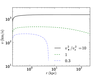
Figure 1.— The wind velocity in the supersonic regime for the solution with Navarro-Frenk-White dark matter halo. The reference mass used is $M_{h}=10^{12}{\rm M}_{\odot}$. The solid, dashed and dotted line are for $v_{\star}^{2}/v_{s}^{2}=10,1,0.3$ respectively. The x-axis starts at $r=R=200$ pc and ends at the virial radius of the halo.

In figure 1 we plot the supersonic wind velocity for a reference halo mass $M_{h}=10^{12}$ $M_{\sun}$ with other NFW parameters calculated using definitions in §3.1 at $z=0$. The value of $v_{s}=236$ km s^-1for this halo. The solid line is for $v_{\star}^{2}=10v_{s}^{2}$ and in this case the injection is large so that the gravity of the halo does not affect the flow. That is why the solid line leaves the plot window and the wind velocity at largest distance is $\approx 1500$ km s^-1which is double the value at $r=R$ in agreement with the result $v_{\infty}=2v_{\star}$ of previous section on the solution of CC85. The dashed line represents the case 2 when $v_{\star}=v_{s}$ and the NFW gravity is important. Consequently the velocities are reduced and at the virial radius, we get a wind velocity $\sim 200$ km s^-1. The dotted line is for $v_{\star}^{2}=0.3v_{s}^{2}$ and it represents the case 3 discussed above. This line exhibits the flow which ends inside the galactic halo at a final radius, $r_{\scriptscriptstyle\rm F}\sim 50$ kpc. We find that for the low $v_{\star}$ values, which implies a low value of velocity at the critical point, the gas stops at some point within the halo. We note that similar solutions were obtained by Wang (1995) for power-law potential, and for specific values of wind speed and mass loss rate, but the calculations were done numerically. The analytical model presented here generalizes these solutions to NFW halo and to general values of wind speed.

4. Injection parameters and value of ${{v}}_{\star}$

In the last section we discussed the importance of the ratio, $v_{\star}^{2}/v_{s}^{2}=\dot{E}/(2\dot{M}v_{s}^{2})$. Here we would like to determine the possible values of $v_{\star}$ which we will use for the rest of the analysis. We can define the energy injection from supernovae per unit time as $\dot{E}=\alpha f_{SN}\dot{M}_{\star}\times(10^{51}\ {\rm erg})$ where $10^{51}$ erg is the energy output of a single supernova, $\alpha$ is the fraction of this energy retained by the gas after radiative energy losses, $\dot{M}_{\star}$ is the SFR in solar mass per year and $f_{SN}$ stands for energy injection per year per solar mass of star formation. For a Kroupa-Chabrier IMF, $f_{SN}\sim 1.26\times 10^{-2}$. Therefore we have,

$$\dot{E}\approx\left[\alpha\ \dot{M}_{\star}\ (4\times 10^{41})\right]\ {\rm erg}\ {\rm s}^{-1}$$ (21)

The mass injection rate is written as

$$\dot{M}=\beta\mathcal{R}_{f}\dot{M}_{\star}$$ (22)

Where $\mathcal{R}_{f}$ is the return-fraction. Typically 30% of the mass is returned to the ISM hence $\mathcal{R}_{f}\approx 0.3$. The factor $\beta$ takes into account the entrainment of mass from ISM which can increase the overall mass injection. For the starburst galaxy M82, $\beta$ is in the range 1.0 to 2.8 which gives $\dot{M}\sim$ 1.4 – 3.6 ${\rm M}_{\odot}\ {\rm yr}^{-1}$ (Strickland & Heckman 2009). Martin (1999) found that for a range of galaxies from low to high masses the mass loss rate roughly scales with SFR . We therefore use $\dot{M}\sim\dot{M}_{\star}$, which corresponds to $\beta\mathcal{R}_{f}\sim 1$ .

With these value of $\dot{E}$ and $\dot{M}$ we estimate the value of $v_{\star}$ which is $(\dot{E}/2\dot{M})^{1/2}=562\sqrt{\alpha}$ km s^-1. We consider two modes of energy injection from SNe. In the first case, almost 90% of the energy of SNe is lost via radiation and only a small fraction goes into heating of the wind. For this ’quiescent mode’, we use $\alpha=0.1$ which gives $v_{\star}\approx 180$ km s^-1. In the other case, when the central injection region is dense and the supernovae are overlapping so that radiative losses reduce, and due to thermalization, 30% to 100% of the supernova energy goes in heating the wind (Strickland & Heckman 2009). This type of situation is evident in galaxies like M82 where the SFR is generally high and the injection regions are supposedly quite dense. For such a case $\alpha=0.3\ \mbox{--}\ 1.0$ and we get $v_{\star}\approx 308\ \mbox{--}\ 562$ km s^-1. To represent this mode we take $v_{\star}=500$ km s^-1. We will call this the ’starburst mode’.

The values of $v_{\star}$ chosen here brackets the range of the possible values. We emphasize that this range of $v_{\star}$, when equated with sound speed corresponds to a temperature range of roughly $\sim 0.2\ \hbox{--}\ 1$ keV, which is consistent with the hot wind temperatures observed in a wide range of galaxies (Martin 2005). On the other hand the quiescent mode ($v_{\star}=180$ km s^-1) is suitable for the galaxies with low values of SFR, like our own Galaxy. This particular mode also yields interesting results, and we will discuss the implications in a later section.

5. Winds in the presence of AGN

The AGN is important as it gives a strong momentum injection to the gas via its radiation field. A large fraction of AGNs show the evidence of outflowing gas, and it is possible that all AGNs drive outflows and they are observed when they are viewed edge-on. Theoretically, these outflows have been associated with the co-evolution of black holes and the bulge of the host galaxy (Silk & Rees 1998; King 2003, 2005). How the AGN interacts with the ISM of the host galaxies and whether it can drive a large scale outflow which can escape the galaxy is an important question. AGN can affect the gas in the host galaxy indirectly where it produces fast nuclear winds which shock the ISM into shells. The fate of these shells is then decided by the supply of energy and momentum injection from the inner regions. Apart from this indirect way AGN can also interact with the dust-rich ISM directly via its radiation field. This interaction is capable of driving large scale outflows (Murray et al. 2005). Here we consider this mechanism and model the outflows as being driven by (Eddington limited) continuum radiation from the black hole.

5.1. Effect of momentum injection from AGN

Momentum injection can be provided by the AGN in several ways. Firstly it can be provided via the scattering of photons by the free-electrons. As the Thompson opacity is generally small ($\kappa_{T}\approx 0.34$ cm² gm^-1 for a fully ionized gas with solar metallicity), this may be effective in the regions close to AGN where the densities are quite large and the radiation field is strong. Another way momentum is transferred to produces outflows is via line driving mechanism (Murray et al. 1995; Proga et al. 2000). We consider the momentum injection via the absorption and scattering of AGN radiation by dust grains. Dust opacities are rather high and recent models of momentum driving of outflows due to AGNs and galactic radiation as well, consider the scattering of photons by dust grains. The gas is assumed to be coupled to these grains through momentum coupling, and get dragged. We justify this assumption in Appendix E.

Let us derive the force due to momentum injection by AGN radiation ($f(r)$) which then will be substituted in equation 4. In its general form, the momentum injection from a radiation field can be written as,

$$f(r)=\kappa\frac{\bf\mathcal{F}}{c}$$ (23)

where $\kappa$ is the volume averaged opacity, ${\mathcal{F}}$ stands for the frequency integrated flux of radiation and c is the speed of light. For spherical symmetry and for a optically thin atmosphere, the radiation flux can be written as $\mathcal{F}=L/4\pi r^{2}$. Hence the force of radiation becomes $\kappa L/4\pi r^{2}c$. This force has an inverse square dependence on r, hence it can be represented as a factor ($\Gamma$) times the gravitational force of the black hole. Therefore, if the gravity of the central black hole is given by $f_{grav}=-GM_{\bullet}/r^{2}$ then in the presence of an outward radiation force, the effective force is written as $f_{g,eff}=-{(1-\Gamma)GM_{\bullet}/r^{2}}$ with $\Gamma=\kappa L/(4\pi GM_{\bullet}c)$. For $\Gamma=1$, the effective force is zero, and for the case of Thompson scattering the corresponding luminosity is called the Eddington luminosity ($L_{E}$). The luminosity required to exactly cancel the gravitational force may be different depending on the opacity and process responsible for momentum injection. For example, in case of scattering of UV light by dust, for which the opacity is roughly 3500 times the electron-scattering opacity (Draine 2003), only a luminosity of $\sim 0.001\ L_{E}$ is required to counter the black hole gravity. However, it has been showed recently that most of the UV photon field from the AGN may get attenuated within a short distance because of the large optical depths in AGN environments (Novak et al. 2012). In that case the re-radiated Infrared(IR) photons serve as the mainstay of AGN radiation (see also Dorodnitsyn et al. (2011). Therefore in this work we consider the momentum injection from IR radiation. IR to dust scattering opacity is, $\kappa_{IR}=13$ cm² gm^-1, in K band (Li & Draine 2001; Draine 2003) for a gas to dust ratio of 125. Opacity in IR is not as large as it is in UV, however we find that it is large enough to drive strong outflows in massive galaxies. Hence the momentum injection force in our case becomes,

$$f(r)={\kappa_{IR}L\over 4\pi r^{2}c}=\Gamma{GM_{\bullet}\over r^{2}}$$ (24)

where $\Gamma=\kappa_{IR}L/(4\pi GM_{\bullet}c)$. We consider an Eddington limited AGN ($L=L_{E}$), where $L_{E}=(4\pi GM_{\bullet}c/\kappa_{T})$ is the usual Eddington luminosity for electron scattering. This fixes the value of $\Gamma={\kappa_{IR}/\kappa_{T}}\approx 38\,$, for our case.

We need to justify that the atmosphere is optically thin in IR so that we can work with a constant $\Gamma$. In order to do this we estimate the optical depth for IR light. Optical depth can be estimated as, $\tau\sim\int\kappa\rho(r)dr$. Using $\kappa_{IR}=13$ cm² gm^-1 and $\rho\sim 10$ m_p cc^-1which, as we will see is an upper limit for density in our wind models, the optical depth comes out to be $0.01$ at $20$ pc and $0.13$ at $200$ pc. Even at the edge of the injection region the optical depth is very small, hence we conclude that the atmosphere is optically thin to IR radiation. Beyond $200$ pc, the density decreases rapidly, as the wind expands adiabatically in the supersonic regime. As we will see in next section, density becomes as low as $0.001$ m_p cc^-1 at $10$ kpc, hence the wind material stays optically thin to IR radiation at large distances as well.

Let us consider the supersonic section of the wind in which both SNe and AGN radiation are effective. (See Appendix B for the subsonic part of this wind.) For the supersonic part the energy and the mass injection both are zero, although the gravity due to NFW halo and the effective force due to radiation and gravity from the central AGN are present. The total potential can be written as,

$$\Phi_{total}(r)=\Phi_{\bullet}(r)+\Phi_{\rm NFW}(r)=-{GM_{\bullet}\over r}-2v_{s}^{2}\ \frac{\ln(1+r/r_{s})}{r/r_{s}}$$ (25)

With the aid of this total potential and the momentum injection term $f(r)=\Gamma{GM_{\bullet}/r^{2}}$, the wind equation 4 for supersonic part ($r>R$) can be written as,

$$\frac{\mathcal{M}^{2}-1}{\mathcal{M}^{2}[(\gamma-1)\mathcal{M}^{2}+2]}\frac{d\mathcal{M}^{2}}{dr}=\frac{2}{r}-\frac{2}{\epsilon(r)}\left({(1-\Gamma)GM_{\bullet}\over r^{2}}+\frac{d\Phi_{NFW}(r)}{dr}\right)$$ (26)

Next we integrate the energy equation directly as below,

$$\left.\epsilon(r)-{(1-\Gamma)GM_{\bullet}\over r}+\Phi_{NFW}(r)\right|_{R}^{r}=0$$

$$\Rightarrow \epsilon(r)=\left[2v_{\rm crit}^{2}-2(1-\Gamma)v_{\bullet}^{2}+\Phi_{\rm NFW}(R)\right]+2(1-\Gamma)v_{\bullet}^{2}{R\over r}-\Phi_{\rm NFW}(r)$$ (27)

where we have used $\epsilon(R)=2v_{\rm crit}^{2}=2v_{\star}^{2}-(1-\Gamma)v_{\bullet}^{2}$, from Appendix B for the subsonic section of this wind. We have also used $v_{\bullet}^{2}=GM_{\bullet}/2R$. The term inside the square bracket in the above equation is a constant, so if we substitute eq 27 in 26 it becomes exactly integrable and we get,

$$\ln\left|\delta_{>}(\mathcal{M})\right|=2\ln\left|r\right|+2\ln\left|2v_{\rm crit}^{2}-2(1-\Gamma)v_{\bullet}^{2}+\Phi_{\rm NFW}(R)+2(1-\Gamma)v_{\bullet}^{2}{R\over r}-\Phi_{\rm NFW}(r)\right|+const.$$ (28)

Using the condition, $\delta_{>}(\mathcal{M})=1$ at $r=R$, and substituting the expression for NFW potential we get,

$$\delta_{>}(\mathcal{M})=(r/R)^{2}\left[1-(1-\Gamma){v_{\bullet}^{2}\over v_{\rm crit}^{2}}\left(1-{R\over r}\right)-{v_{s}^{2}\over v_{\rm crit}^{2}}\left(\frac{\ln(1+R/r_{s})}{R/r_{s}}-\frac{\ln(1+r/r_{s})}{r/r_{s}}\right)\right]^{2}$$ (29)

where $v_{\rm crit}^{2}=v_{\star}^{2}-(1-\Gamma)v_{\bullet}^{2}/2$. This equation gives the complete solution of the wind from a galaxy driven by energy injection from SNe and momentum injection from the AGN. Let us discuss some asymptotic behaviours,

• Terminal speed :
  We use the Bernoulli equation 27 to obtain the terminal speed. Taking the limit $r\rightarrow\infty$ in equation 27 and neglecting the sound speed we obtain the following general expression for terminal speed of SNe and AGN driven wind from a NFW halo,

  $$v_{\infty}=2\left(v_{\star}^{2}+\frac{3}{2}(\Gamma-1)v_{\bullet}^{2}-v_{s}^{2}\right)^{1/2}$$ (30)

  Here $v_{s}^{2}=GM_{h}/(2\mathcal{C}r_{s})$. In the absence of dark matter halo and the AGN we can neglect $v_{s}$ and $v_{\bullet}$ which gives $v_{\infty}=2v_{\star}$. However in presence of NFW gravity but no AGN we get the relation $v_{\infty}=2\sqrt{v_{\star}^{2}-v_{s}^{2}}$. For dwarf galaxies, the effect of NFW gravity can be neglected, and therefore the wind speed in starburst mode is expected to be $v_{\infty}\approx 1000$ km s^-1, consistent with observations of winds in starburst galaxy M82 (catalog ). If the black hole is massive so that the $v_{\bullet}$ dominates then by neglecting $v_{\star}$ and $v_{s}$ and putting $\Gamma=38$, we get $v_{\infty}\approx 15v_{\bullet}$, which for a black hole of mass $\sim 10^{9}$ ${\rm M}_{\odot}$ estimates to $v_{\infty}\sim 1500$ km s^-1.

• Behaviour with r :
  In equation 29 if the SNe injection term ($v_{\star}$) is dominant then we get $\mathcal{M}^{3}\propto r^{2}$. When the wind is moving with constant terminal speed, $T\propto r^{-4/3}$ and $\rho\propto r^{-2}$ as derived in §2.1. If the AGN provides the main driving then neglecting $v_{s}$ and $v_{\star}$ from equation 29, for large r, we once again retain $\mathcal{M}^{3}\propto r^{2}$, and hence the scaling $T\propto r^{-4/3}$. The density scales as $\rho\propto r^{-2}$.

It is clear that, apart from the $v_{\star}$, the wind properties depend on two more terms. One involves $v_{\bullet}$ which is a parameter of the black hole and the other being $v_{s}$, which depends on the mass of NFW halo. To proceed further we need to learn whether the black hole mass is somehow related to dark matter halo.

Observations show that the black hole mass is related to the velocity dispersion of the central spheroidal bulge component of the galaxies, and the relation can be written as

$$\log\left({M_{\bullet}\over{\rm M}_{\odot}}\right)=a+b\log\left({\sigma\over 200\ {\rm km\ s^{-1}}}\right)$$ (31)

This correlation has been extensively studied in the literature, with slightly different values for $a$ and $b$. We will list a few of them. Gebhardt et al. (2000) was one of the earliest to report the correlation with $a\simeq 8.08\pm 0.07$ and $b=3.75\pm 0.3$. Ferrarese (2002) gives $a\simeq 8.22\pm 0.08$ and $b=4.58\pm 0.52$. Values in Tremaine et al. (2002) reads $a=8.13\pm 0.06$ and $b=4.02\pm 0.32$. For our analysis we use $a=8.12$ and $b=4.24$ from a recent study by Gültekin et al. (2009).

We also use a relation between the $\sigma$ and circular speed $v_{c}$. Ferrarese (2002) reported a correlation between the circular speed in outskirts of galaxy and the $\sigma$, given roughly as $v_{c}\propto\sigma^{0.84\pm 0.09}$. Similar relations were also deduced by Baes et al. (2003) and Pizzella et al. (2005). All these relation are very close to the linear relation $v_{c}=\sqrt{2}\sigma$ for spherical mass distribution (Binney & Tremaine 2008), found in massive ellipsoidal galaxies where the bulge to total mass ratio is unity (see also Volonteri & Stark 2011). Hence for our analysis we use $v_{c}=\sqrt{2}\sigma$.

The relation between $v_{c}$ and $\sigma$ breaks down for low mass galaxies (Ferrarese 2002). It is easy to understand this as the lower mass galaxies may admit a bulge to total mass ratio less than unity. Hence the galaxies with smaller bulges will have the mass of their black holes smaller than the one expected from $M_{\bullet}\hbox{--}\sigma\hbox{--}v_{c}$ relation. On similar grounds, Kormendy & Bender (2011) concluded against the co-evolution of central black hole and dark matter halo. However, they also showed that a cosmic conspiracy causes $v_{c}$ to correlate with $\sigma$ for massive galaxies ($v_{c}\gtrsim 200$km s^-1).

We would like to emphasize here that even if the $v_{c}\hbox{--}\sigma$ relation breaks down below a $v_{c}\lesssim 200$ km s^-1, still it does not make a difference in our results because the AGN term is effective only for very massive systems. In equation 26 it is the relative values of $v_{\bullet}$ and $v_{s}$, which govern the dynamics. For $v_{c}$=200 km s^-1, using $c=12$ we get $v_{s}=(GM_{h}/2\mathcal{C}r_{s})^{1/2}\approx 400$ km s^-1which is larger than $(\sqrt{\Gamma-1})v_{\bullet}\approx 100$ km s^-1, and the black hole term is even smaller for $v_{c}<200$ km s^-1.

Using the $M_{\bullet}\hbox{--}\sigma$ relation provided by Gültekin et al. (2009), aided with the relation $\sigma=v_{c}/\sqrt{2}$, where $v_{c}$ is given by equation 11 we arrive at the following relation between black hole mass and the halo mass (see also Volonteri & Stark (2011)).

$$\left(M_{\bullet}\over 0.74\times 10^{7}\ M_{\odot}\right)^{1/\sqrt{2}}\simeq\ \left({M_{h}\over 10^{12}\ {\rm M}_{\odot}}\right)\left[{\Omega_{m}\over\Omega_{m}^{z}}{\Delta_{c}(z)\over 18\pi^{2}}\right]^{1/2}(1+z_{\rm vir})^{3/2}$$ (32)

where $z_{\rm vir}$ is the redshift at which the halo collapsed and got viriallized. This relation can be used to determine $v_{\bullet}$ as a function of halo mass through, $v_{\bullet}=(GM_{\bullet}/2R)^{1/2}$. Substituting $v_{\bullet}$ and $v_{s}=\sqrt{GM_{h}/2r_{s}\mathcal{C}}$ in equation 29 with $r_{s}$ and $\mathcal{C}$ determined from the redshift dependent definitions for NFW parameters given in §3.1. This enables us to compute the mach numbers as a function of $r$ for the galaxy of any desired halo mass($M_{h}$) and its halo collapsing at any desired redshift. The mach numbers can then be converted to the velocity simply by multiplying it with the sound speed which can be obtained using the relation $c_{s}^{2}=\epsilon(r)/(\mathcal{M}^{2}/2+1/(\gamma-1))$.

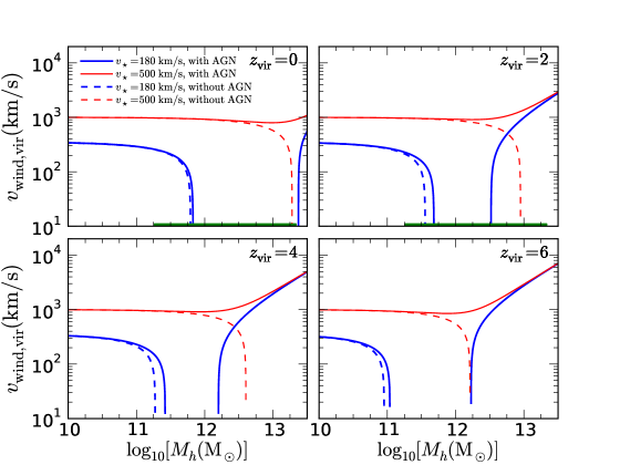
Figure 2.— Wind velocity at virial radius as a function of halo mass for four different redshifts of collapse, $z_{\rm vir}=0,2,4,6$ in the panels from top-left to bottom-right respectively. The thin red lines in each panel are for starburst mode ($v_{\star}=500$ km s^-1) and thick blue ones are for quiescent mode ($v_{\star}=180$ km s^-1). Dashed line represent the outflow speeds without AGN. The green bar on x-axis in top two panels gives the range of galaxies in which the gas reservoirs in halos are observed (Tumlinson et al. 2011).

In figure 2 we plot the wind velocities at virial radius ($v_{\rm wind,vir}$) as a function of halo mass($M_{h}$). The velocities are obtained by solving equation (29) with inputs from equation 32 and definitions in section 3.1. We show the results corresponding to four different value of $z_{\rm vir}$ in four panels. red lines are for the starburst mode $v_{\star}=500$ km s^-1and the blue lines are for the quiescent mode $v_{\star}=180$ km s^-1. The dashed lines represent the solution without AGN and these show that the wind velocities cut of at some halo mass as the gravity becomes strong enough to counter the energy injection. For larger value of $v_{\star}$ this cut-off occurs at a larger halo mass.

Consider a situation in which for low halo masses the AGN driving term is smaller than the NFW gravity term. This implies that the wind velocity at virial radius in low mass halos decreases with increase in halo mass. However the black hole mass also increases with the halo mass. Since the slope of $M_{\bullet}\hbox{--}M_{h}$ relation is greater than unity, hence the rate of increase of the black hole or AGN term is larger and at a particular halo mass it overcomes the NFW gravity term. Hence for largest galaxies we should see an increase in wind velocity with halo mass, which indeed is the case as shown by rising solid lines for massive halos. One can further compare the solid lines with dashed lines where the latter represent the case without the AGN and does not show any winds in high mass galaxies, which is a confirmation of the fact that in high mass galaxies outflows are driven by AGN.

The thick solid blue curve is special as it features the wind quenching due to NFW gravity as well as the high velocity winds due to AGN. There is a falling part of the curve which exhibits the cut off at some halo mass and then there is another part which rises at some larger halo mass. Hence there exist a range of halo masses roughly within $10^{11\hbox{--}13}{\rm M}_{\odot}$, which do not have escaping winds. The exact value of this range depends on the redshift of collapse ($z_{\rm vir}$). For example at $z_{\rm vir}=0$ the rising part of the thick blue curve, which shows the effect of AGN, starts rising beyond a halo mass of $10^{13}{\rm M}_{\odot}$ while for $z_{\rm vir}=2$ it rises roughly at a halo mass $\sim 10^{12}{\rm M}_{\odot}$. This is easy to understand as the AGN driving depends on the black hole mass which does increase with redshift (see equation 32). Also the falling part of the thick blue curve ends at a smaller halo mass for a larger value of $z_{\rm vir}$, because the value of $v_{s}$ increases with redshift. We would like to mention here that the recent detection of gas reservoirs in the halos of galaxies by Tumlinson et al. (2011) covers roughly the similar range in halo masses shown by the green bar on x-axis in upper two panels of figure 2.

If we focus on the wind velocities in lower to intermediate mass halos $M_{h}<10^{12}{\rm M}_{\odot}$, we find that AGN never dominate in these and if there are winds they have to be driven by starbursts and SNe. We note that the wind velocities in low mass galaxies fall in the range $400\hbox{--}1000$ km s^-1, depending on the efficiency of the energy injection process. These velocities agree with the ones inferred from the X-ray temperatures of the superwind regions in dwarf straburst and luminous infrared galaxies (Heckman et al. 2000; Martin 1999). However in case of galaxies with halo mass, $M_{h}\gtrsim 10^{12.5}{\rm M}_{\odot}$ the wind velocities either exceed 1000 km s^-1or they are quenched, depending on whether the AGN is present or not.

We note that in low mass galaxies where the outflows are driven by SNe, the wind velocity, $v_{\rm wind}\lesssim 1000$ km s^-1. However this limit is exceeded when an AGN is present, since the curves with AGN show wind velocities $\gtrsim 1000$ km s^-1. This reveals the presence of a dividing line of 1000 km s^-1between SNe and AGN domination in velocity space as well.

In a hot wind with velocity of $v_{\rm wind}$ the neutral clumps in the wind can be dragged via the ram pressure. Maximum velocity these clouds can achieve is the velocity of the hot wind. As mentioned above, $v_{\rm wind}$ is always within 1000 km s^-1at the low mass end where SNe injection dominates, therefore the cold clouds should also be outflowing with velocity lower than 1000 km s^-1. On the other hand at the higher mass end, where the AGN dominates, the velocities may exceed this limit. Interestingly, the observed outflow speeds of the neutral clouds in diverse galaxies like dwarf starbursts, ULIRGs, post-starburst galaxies and Low-ionization BAL quasars also follow this trend (Tremonti et al. 2007; Sturm et al. 2011; Trump et al. 2006).

It has been debated in the literature that the neutral cold/warm winds in ULIRGs are driven by ram pressure of the hot wind and/or radiation from stars in the galaxy or by the AGN. If we consider the winds driven by stellar radiation then the wind speed is roughly 3 times the circular speed of the galaxy (Murray et al. 2005; Martin 2005; Sharma et al. 2011). For a massive ULIRG with a circular speed $\sim 300$ km s^-1the wind velocity predicted by radiation driven wind model will be $900$ km s^-1. On the other hand, if ram pressure is the driving mechanism, then also the velocities of the continuous hot wind and hence of the neutral clouds can not exceed 1000 km s^-1unless an AGN is present. Therefore we emphasize that the observations of wind velocity in excess of 1000 km s^-1indicate the presence of an AGN.

5.2. Wind properties with distance : Implications for gas observed in galactic halos

In the last section we have established that for a particular mass range the galactic winds may not escape the galaxy. Therefore these galaxies are not very important for the intergalactic medium (IGM) enrichment. Interestingly our Milky Way with a total mass roughly $\sim 10^{12}{\rm M}_{\odot}$, also falls in this mass range. However an important question arises for these type of galaxies, as to whether or not these galaxies can retain all the gas in the disk even though they can contain the gas inside $r_{\rm vir}$.

Figure 3.— The wind properties as a function of distance from the base. Legend is same as in figure 2. From left to right, the three columns correspond to three different halo masses, representing a dwarf galaxy, a Milky Way size galaxy and a giant galaxy respectively. The x-axis in all the plots extend upto the corresponding virial radius. The solid lines represent the winds in presence of an Eddington limited AGN and the dashed lines, the case of no AGN. Thin red lines represent the starburst mode ($v_{\star}=500$ km s^-1) and the thick blue lines are for the quiescent mode ($v_{\star}=180$ km s^-1). The middle row contains the temperature profiles of winds in three galaxies. The lowermost row shows the densities. To calculate densities we have used $\dot{M}_{\star}=1,3,10$ ${\rm M}_{\odot}$ yr^-1 for $v_{\star}=180$ km s^-1, and $\dot{M}_{\star}=10,30,100$ ${\rm M}_{\odot}$ for $v_{\star}=500$ km s^-1, for three galaxies respectively.

We show in this section that infact these galaxies have outflows which spill their gas reservoir throughout the halo. In figure 3 we show the radial dependence of wind properties for three galaxies which differ in the values of their halo mass. We have considered the halos collapsing at a redshift of $z_{\rm vir}=2$ which corresponds to a look-back time of roughly $\sim 10$ Gyr. We choose this collapse redshift, as a fiducial value, in order to model galaxies like Milky Way and more massive galaxies, whose halos were already in place by $z\sim 2$. The thick disk in our Galaxy shows that Milky Way underwent its last major merger before $\sim 10$ Gyr, which corresponds to $z\sim 2$ (Gilmore et al. 2002). Therefore our results can be compared with observations of winds at low redshift ($z\leq 2$) universe.

In figure 3, the thick blue lines refer to the quiescent mode ($v_{\star}=180$ km s^-1) and the thin red lines represent the starburst mode ($v_{\star}=500$ km s^-1). The solid lines denote the effect of AGN activity and dashed lines consider only the SNe injection. The upper panels plot the velocity as a function of radius, and the middle and bottom panels plot the temperature and densities respectively. The densities are estimated using the relation $\rho=\dot{M}/4\pi vr^{2}$, where $\dot{M}\sim\dot{M}_{\star}$. For three galaxies with $M_{h}=10^{11},10^{12},10^{13}{\rm M}_{\odot}$, we have used $\dot{M}_{\star}=1,3,10$ ${\rm M}_{\odot}$yr^-1 for quiescent mode and $\dot{M}_{\star}=10,30,100$ ${\rm M}_{\odot}$yr^-1 for starburst mode respectively.

The curves show that for low mass galaxies, all types of winds (with or without AGN, quiescent and starburst mode) escape the virial radius. At the other extreme, for massive galaxies, winds with AGN activity can escape, but without an AGN, they stop at a distance within the halo ($\sim 10\hbox{--}200$ kpc). The gas temperature and density slightly rises at this final halting point due to adiabatic compression. We would like to mention here that the radiative cooling can be important for these particular cases as the steady solution ceases to exist beyond a point. Even if the cooling time is shorter than the flow time initially, after many flow crossing times the cooling will become effective which may cause thermal instability. This can lead to formation of clouds whose fate then will be decided by the physical properties in their environment (see also Wang 1995).

For the intermediate mass galaxy ($M_{h}\sim 10^{12}{\rm M}_{\odot}$), we find that both of the thick blue lines (i.e., quiescent mode of star formation with or without AGN) are contained inside the virial radius. This implies that the wind needs strong starburst activity in order to escape the galaxy irrespective of whether or not AGN is present. The dashed thick blue line corresponds to a quiescent mode of star formation without AGN and roughly corresponds to our own Galaxy. Interestingly, we find that a slow wind is possible, which may extend to a distance of $\sim 20$ kpc. This can explain the recent observations of clouds roughly at $10\hbox{--}20$ kpc in our halo (Keeney et al. 2006).

The solutions which end inside $r_{\rm vir}$ are important in the wake of recent observation of warm-hot gas clouds in the halo of our galaxy and for other galaxies as well (Tumlinson et al. 2011). Also recent simulations confirm these gas reservoirs around the galaxies of intermediate masses. Recent works find that although in the general scenario of galaxy formation the intermediate mass galaxies are efficient in retaining their baryons, these galaxies do not retain all of the baryons. It appears that only 20% to 30% of baryons are converted to stars in these galaxies as well (Somerville et al. 2008; Moster et al. 2010; Behroozi et al. 2010). Our results provide a natural explanation for the missing baryons in these intermediate mass galaxies.

5.3. Cosmological implications

Here we derive a relation between the stellar mass and the halo mass using the results for SNe and AGN driven outflows in the previous section. In the the scenario of hierarchical structure formation low mass galaxies form at earlier times and post formation history is influenced by mergers and the periods of enhanced star formation activity. The semi-analytical modeling (SAM)(see Baugh 2006), which uses simple recipes for feedback and follows the structure formation according to $\Lambda$CDM model, can explain the observed properties of galaxies (Somerville et al. 2008). In recent years there have been a growing amount of observational evidence that the massive black holes were already in place at high redshifts. Also, it is well accepted that the massive galaxies formed their stars at earlier epochs as they appear redder at present times, compared to the younger galaxies in which star formation is still going on (Fontanot et al. 2009, and references therein). This phenomenon, which are commonly referred as ’downsizing’, indicate a possible role the massive black holes would have played in quenching the star formation in massive galaxies at earlier epochs (Somerville et al. 2004; Granato et al. 2004; Croton et al. 2006). We follow the semi-analytical scheme proposed in Granato et al. (2004) for which an approximate analysis is provided in the appendix A of Shankar et al. (2006), using which, we can write the rate of change of cool gas in halos as,

$$\dot{M}_{cold}(t)=\frac{M_{infall}(t)}{t_{c}}-\dot{M}_{\star}(t)+\mathcal{R}_{f}\dot{M}_{\star}(t)-\mathcal{L}\dot{M}_{\star}(t)\,,$$ (33)

where $\mathcal{R}_{f}$ is the return fraction of stars whose value is $0.3$ for a Salpeter IMF. $\mathcal{L}\dot{M}_{\star}$ is the mass loss rate, $t_{c}$ is the cooling time. $M_{infall}(t)$ is the mass available in the halo for infall at a time $t$ . The Equation 33 can be solved to obtain a time independant solution in large time limit and yields a stellar mass at present epoch as (see eqn 17 in Shankar et al. 2006),

$$M_{\star}=f_{surv}\frac{f_{cosm}M_{h}}{1-\mathcal{R}_{f}+\mathcal{L}}\,,$$ (34)

where $f_{cosm}=1/6$ is the cosmic baryon ratio, $f_{surv}$ is the fraction of stars surviving up to now and its value is approximately $0.6$ for a Salpeter IMF. As $f_{surv},\ f_{cosm}$ and $\mathcal{R}_{f}$ are constants, therefore we get $M_{star}\propto M_{h}/\mathcal{L}$. In case of SNe feedback the feedback factor is written as $\mathcal{L}=\frac{\alpha f_{SN}(10^{51}\,{\rm erg})}{E_{bind}}$, where $E_{bind}=[v_{c}^{2}f(c)(1+f_{cosm})/2]$ with $f(c)$ as given in Mo et al. (1998), represent the binding energy of gas in the halo per unit mass. The quantity in the numerator is nothing but $\dot{E}/\dot{M}=2v_{\star}^{2}$ where $v_{\star}$ is the value of velocity at the critical point for the case of only SNe injection and no AGN. When the AGN is also present we can use the modified value of velocity at the critical point given in equation 27 which is $v_{\rm crit}^{2}=v_{\star}^{2}-(1-\Gamma)v_{\bullet}^{2}/2$. Hence in the case of both SNe and AGN feedback we can write the loss term $\mathcal{L}$ as,

$$\mathcal{L}=\frac{2v_{\rm crit}^{2}}{{1\over 2}v_{c}^{2}f(c)(1+f_{cosm})}=\frac{2[v_{\star}^{2}-({1-\Gamma\over 2})v_{\bullet}^{2}]}{{1\over 2}v_{c}^{2}f(c)(1+f_{cosm})}$$ (35)

$v_{\rm crit}$ is the velocity at the critical point and $v_{c}$ the virial velocity of the halo. While the velocity at the critical point measures the strength of SNe and/or AGN as a mechanism of mass expulsion, the velocity at the virial radius is a measure of binding energy of the halo.

For NFW halo, $v_{c}\propto M_{h}^{1/3}$. Also $v_{\bullet}^{2}\propto M_{\bullet}\propto M_{h}^{1.41}$ (see equation 32). Using these we get

$$M_{\star}\propto\frac{M_{h}}{1-\mathcal{R}_{f}+{4v_{\star}^{2}+CM_{h}^{1.41}\over DM_{h}^{2/3}}}\propto\frac{M_{h}^{5/3}}{A+CM_{h}^{1.41}}$$ (36)

where $C$, $D$ are constants and $A=[0.8f(c)v_{c}^{2}+4v_{\star}^{2}]$. From the above relation we find that for small halo masses we have $M_{\star}\propto M_{h}^{5/3}$ and for large halo masses, when the AGN dominates, we get $M_{\star}\propto M_{h}^{0.26}$. The break occurs and $M_{\star}/M_{h}$ peaks roughly in the range $\sim 10^{12\hbox{--}12.5}{\rm M}_{\odot}$ as the ratio $v_{\rm crit}^{2}/v_{c}^{2}$ becomes minimum around this mass.

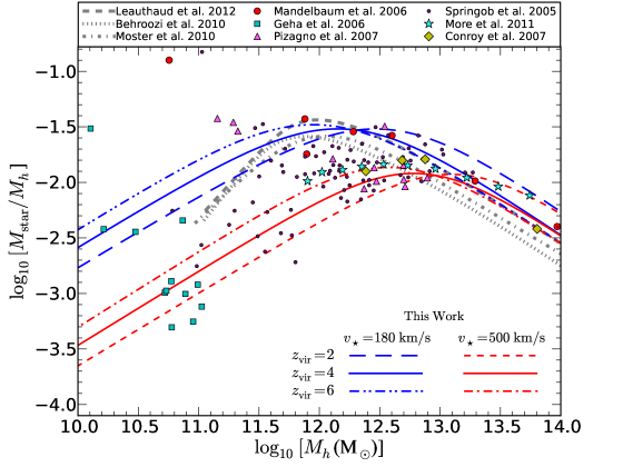
Figure 4.— SHMR at present time from theoretical considerations in this work is compared with the observational data for individual galaxies courtesy Alexie Leauthaud. The upper three (blue) lines represent the quiescent mode ($v_{\star}=180$ km s^-1) and the lower three (red) lines represent the starburst mode ($v_{\star}=500$ km s^-1) of galaxies. In these the dashed, solid and dash-dotted lines correspond to collapse redshifts, $z_{\rm vir}=2$, 4 and 6 respectively. The data points are from Mandelbaum et al. 2006 : filled red circles, Geha et al. 2006:filled green squares, Pizagno et al. 2007 : filled purple triangles, Springob et al. 2005 : dots, More et al. 2011 : stars, Conroy et al. 2007 : diamonds. The thick gray dashed, dotted and dash-dotted lines represent the results of halo abundance matching from Leauthaud et al. (2012), Behroozi et al. (2010) and Moster et al. (2010) respectively.

In Figure 4, we plot the SHMR at present day, against the halo mass obtained by using equation 34, 35 and 32. The set of upper three blue lines correspond to quiescent mode ($v_{\star}=180$ km s^-1) and the lower three red line represent the starburst mode ($v_{\star}=500$ km s^-1). In each set the dashed, solid and the dash-dotted lines correspond to three different redshifts of collapse, $z_{\rm vir}=2$, 4 and $6$ respectively. We stress here that the lines denote the value of SHMR at present day ($z=0$) for the galaxies which got viriallized at a particular $z_{\rm vir}$.

The squares, dots, and triangles in Figure 4 represent the stellar and halo mass data inferred from works on Tully fisher relation by Geha et al. (2006), Springob et al. (2005) and Pizagno et al. (2007) respectively. The stars and diamonds represent the data from (More et al. 2011) and (Conroy et al. 2007) who deduced the stellar and halo mass using stellar dynamics. Red circles shows the estimates based on weak lensing by (Mandelbaum et al. 2006). For details on the data sets the reader is referred to Leauthaud et al. (2012) and Blanton et al. (2008) and the original papers for the the data sets. We have also shown the SHMR obtained by the technique of halo abundance matching (Moster et al. 2010; Behroozi et al. 2010; Leauthaud et al. 2012) using broken thick gray lines. At the higher mass end we note that our results agree with these works. To be more specific we find a stellar to halo mass slope of $0.26$ as mentioned above, which is in agreement with the value $0.29$ deduced in Behroozi et al. (2010). The slope at higher mass end depends on the $M_{\bullet}-M_{h}$ relation, which is still being debated in the literature. However, even if we use a different scaling like $M_{\bullet}\propto\sigma^{4.02}$ given by Tremaine et al. (2002), then the slope at high mass end becomes $0.33$ which is also in agreement with observations and other works.

The slope at low mass end as found by halo abundance matching is roughly $\sim 2.2$, which is larger than $5/3$ from theoretical considerations in this work and others (e.g. Dekel & Woo 2003). however, it is possible that other physical processes not considered in our model can explain the discrepancy. For example, if $v_{\star}$ depends on halo mass, with the efficiency of SNe energy injection being larger in low mass halos, the slopes can be reconciled.

If one naively compares the lines from our analytical calculation with the observational data points for individual galaxies then the plot seems to say something interesting. By looking at the data for low to intermediate mass galaxies (Geha et al. 2006; Springob et al. 2005; Pizagno et al. 2007) one may infer that the data points lie systematically below the results of halo abundance matching. There are a lot of galaxies which have lower stellar content than expected from halo abundance matching. However, if we compare these with our lower three red lines which are for starburst mode then these data points can be reconciled. As we have already described, the outflow activity in low to intermediate mass galaxies is governed by SNe and starbursts. The two modes we are following in this paper represent two extreme efficiencies of energy injection by SNe. Quiescent galaxies like ours lie on one extreme and the violent galaxy like M82 on the other extreme. All the galaxies in low to intermediate halo mass range ($\lesssim 10^{12.5}{\rm M}_{\odot}$) are covered between these two extremes. Interestingly in Figure 4 also, most of the data points lie between the blue and red lines of our theoretical model which represent the quiescent and starburst mode of energy injection respectively. This is not mere a coincidence given the simplicity of our model and shows the importance of outflows in shaping the galaxies.

In the above analysis, we have assumed that the relation given in equation 34, which is valid in the long time limit, gives the stellar mass in the present day universe. In the hierarchical structure formation scenario where small halos form first and undergo periods of high merger rates, this assumption may not be completely valid. However, recent observations and theoretical works have shown that cosmic downsizing mitigates the effects of hierarchical structure formation models, and that massive galaxies are believed to form stars at high redshift after which they evolve passively. In this regard, the consistency of our results with observations of massive galaxies becomes important.

6. Discussions

In this paper we have studied galactic outflows driven by SNe injection and AGN radiation. We have calculated the outflow properties in halos ranging from low to high mass. The treatment is analytical which enabled us to extract fundamental results for these feedback processes. Here we recapitulate the results and the caveats.

We have found that the NFW gravity causes the outflows to stop inside virial radius in intermediate to high mass halos. In Appendix C, we have shown the solutions for winds from NFW halo in terms of Mach number, where the closed contours show the importance of the halo. In other words, gravitational force of the halo causes the flow to stop inside the virial radius if the energy injection from SNe is not large. We note that a minimum value of SNe energy injection so as to produce $v_{\star}\sim v_{s}$ is required for the gas to escape the galaxy. Our models in which the gas can not escape the galaxy, provides a natural explanation for the circumgalactic material observed inside the halos and also predict mild winds in quiescent star forming galaxies such as our Galaxy.

When an AGN component is included, the contours in the Mach number–radius plot can open up for massive galaxies ($M_{h}\gtrsim 10^{12.5}{\rm M}_{\odot}$). This implies that AGN radiation can become important in winds from massive galaxies (such as ULIGs), reaching a wind velocity of $v_{\rm wind}\gtrsim 1000$ km s^-1. If we consider that neutral clouds are entrained in this wind then the speeds of the cold clouds can be at the most equal to $v_{\rm wind}$. This result is consistent with observed outflow speeds in post-starburst galaxies, ULIRGs and Low-ionization quasars at intermediate to high redshifts (e.g. Tremonti et al. 2007; Sturm et al. 2011). We have derived a general expression for the terminal speed of the wind from the NFW halo which can be written as $v_{\infty}=(4v_{\star}^{2}+6(\Gamma-1)v_{\bullet}^{2}-4v_{s}^{2})^{1/2}$, where $v_{\star}$ is the contribution from SNe and the term with $v_{\bullet}$ stands for the momentum injection from AGN. According to our results 1000 km s^-1is an upper limit for the starburst driven winds while in case of AGN driving which is possible in high mass galaxies only, the velocities always exceed 1000 km s^-1. We note here that this limit holds for large scale escaping outflows for all galaxies; however there may be exceptional cases where the system is going through a period of extreme star formation, and even without AGN, the wind speed at a few kpc can be more than 1000 km s^-1(Diamond-Stanic et al. 2012). These episodic winds are likely to be driven by the radiation from galaxy as the galaxy becomes highly luminous due to extreme star formation (Sharma et al. 2011).

We have also shown that our results can explain the observed trends of stellar to halo mass ratio. We find that the stellar mass scales with the halo mass as $M_{\star}\propto M_{h}^{0.26}$ at the higher mass end and $M_{\star}\propto M_{h}^{1.67}$ at the lower mass end. The slope at higher mass end agrees with the observations and abundance matching results. We find that the large scatter in observational data at the lower mass end is due to the fact that the efficiency of energy injection is different in different galaxies. We would like to mention here that we have used a simple recipe to calculate the stellar mass corresponding to a particular halo mass using the outputs from our wind models. Implementing feedback recipes from our wind models into a full semi analytical work is beyond the scope of this paper. Also we have assumed spherical symmetry for our calculation which is justified considering the large length scale ($\sim 100$ kpc) of these outflows. However in the vicinity of the disk the effect of gravity due to a flattened system may be important as explored using a self-similar model in Bardeen & Berger (1978). We leave the problem of finding streamlines in a cylindrical geometry for these outflows to a future work.

We note that the reprocessed IR radiation is sufficient to drive strong outflows from high mass galaxies and the resulting feedback is enough to explain the mismatch between stellar mass and halo mass at high mass end. This is important as one need not to rely on UV radiation which is supposed to be attenuated quickly within a small distance from the center.

The injection of energy and mass in our model occurs in the central region. However recent observations show the evidence of outflows emerging from individual star clusters which may be situated away from the center of the galaxies (e.g. Schwartz et al. 2006). It becomes however analytically complicated to take into account the contribution from these clusters and combine it with the effects of a central AGN. It is however clear that effects of the feedback would be higher if mass and energy injection occurs even beyond the central region and from a large number of clusters.

The coupling between gas and dust is shown to be mediated via momentum coupling. However one may question the survival of dust grains. For this we refer to the observational evidence for dust in the spectra of AGNs, which shows that the dust does survive and it may do so by residing in small clumps around AGN as discussed in Krolik & Begelman (1988).

We have considered momentum transfer from AGN radiation in optically thin limit. In actual practice the situation can be quite complicated and it may not be exactly accurate to use a constant $\Gamma$. We hope that the simulations of winds with full radiation transfer covering from small to large length scales will be able to verify the simple ideas presented here. We have used a relation between the black hole mass and the dark matter halo mass. We have projected this relation backward in time using scalings of NFW parameters with redshift. There are observational evidence that black hole masses at high redshifts are generally higher, however it is hard to predict the correct scaling of black hole mass with redshift as the formation and growth of black holes is a complicated problem in itself.

We have not considered the effects of radiative cooling in the present work. Radiative cooling is important for the thermodynamics of the outflow. The CC85 solution with implementation of cooling has been studied in the past (Silich et al. 2004; Tenorio-Tagle et al. 2007; Wünsch et al. 2011; Silich et al. 2011). These calculations conclude that cooling (if not catastrophic) does not affect the velocity and density but causes the temperature to decay more rapidly. Wind solutions with cooling can not be worked out analytically for general values of parameters and one has to use the numerical computation, for particular cases. We have discussed the hot phase of the outflows which is tractable using analytic hydrodynamics. However in actual practice the physics of hot, cold and molecular phase of galactic outflows might be tangled to each other . The study of all these components demands state of the art numerical simulations. We hope to study the multi-phase character of these winds in a future paper.

To summarize, we have found analytical solutions for SNe and AGN driven winds from realistic dark matter halo. Our results show that the two feedback processes operate effectively at two ends of the galaxy luminosity function as expected. The wind velocities for escaping winds resulting from our calculations explains a variety of observations. We find that AGN can drive the gas to speeds $\gtrsim 1000$ km s^-1. We find an intermediate mass range in which the outflows can be highly suppressed and for these halo masses the gas can not escape into the IGM. However, the gas is still driven to large distances within the halo. This result explains the recent observations of gas reservoirs in our Galaxy and other galaxies. Using the results of our analytical models, we have derived a stellar mass to halo mass relation using simple recipes. We find the derived $M_{\star}\hbox{--}M_{h}$ relation matches the results of observations and halo abundance matching. Thus, our findings provide a possible explanation for missing baryons in galaxies.

We thank Mitchell Begelman for critical reading of the manuscript. We are grateful to Alexie Leauthaud for providing the observational data used in Figure 4. We thank Tim Heckman, Rachel Somerville and Prateek Sharma for fruitful discussions. We also thank an anonymous referee for constructive comments.

Appendix A Appendix A: Detailed derivation of wind equation

The equations (1) and (2) can be written as

$${2\over r}+{1\over\rho}{d\rho\over dr}+{1\over v}\frac{dv}{dr}={\dot{m}\over\rho v}$$ (A1)

$$v\frac{dv}{dr}=-{c_{s}^{2}\over\gamma}\left({1\over\rho}{d\rho\over dr}\right)-{1\over\gamma}{\frac{dc_{s}^{2}}{dr}}+f(r)-\frac{d\Phi(r)}{dr}-{\dot{m}v\over\rho}$$ (A2)

where $c_{s}^{2}=\gamma p/\rho$. Elimination of ${1\over\rho}{d\rho\over dr}$ from above two equations yields,

$$v\frac{dv}{dr}-{c_{s}^{2}\over\gamma v}\frac{dv}{dr}=-\frac{1}{\gamma}\frac{dc_{s}^{2}}{dr}+{c_{s}^{2}\over\gamma}\left({2\over r}-{\dot{m}\over\rho v}\right)-{\dot{m}v\over\rho}+f(r)-\frac{d\Phi(r)}{dr}$$ (A3)

from energy equation (Equation 3) we have,

$$v\frac{dv}{dr}+{1\over\gamma-1}\frac{dc_{s}^{2}}{dr}={q\over\rho v}-{\epsilon(r)\dot{m}\over\rho v}+f(r)-{\frac{d\Phi(r)}{dr}}$$ (A4)

where $\epsilon(r)=\frac{v^{2}}{2}+\frac{c_{s}^{2}}{\gamma-1}$. Elimination of $\frac{dc_{s}^{2}}{dr}$ from Equation A3 and A4 results in,

$$\frac{v^{2}-c_{s}^{2}}{v}\frac{dv}{dr}={c_{s}^{2}}\left({2\over r}-{\dot{m}\over\rho v}\right)-(\gamma-1)\left(\frac{q}{\rho v}-\frac{\dot{m}\epsilon(r)}{\rho v}\right)+f(r)-\frac{d\Phi(r)}{dr}-{\dot{m}v\gamma\over\rho}$$ (A5)

Next we introduce the Mach number $\mathcal{M}=v/c_{s}$. We can write the following relations,

$$v\frac{dv}{dr} = \frac{c_{s}^{2}}{2}\frac{d\mathcal{M}^{2}}{dr}+\frac{\mathcal{M}^{2}}{2}\frac{dc_{s}^{2}}{dr}\quad;$$

$${1\over v}\frac{dv}{dr} = \frac{1}{2\mathcal{M}^{2}}\frac{d\mathcal{M}^{2}}{dr}+\frac{1}{2c_{s}^{2}}\frac{dc_{s}^{2}}{dr}$$ (A6)

Using these relations in Equation A4 and A5 we obtain,

$$\frac{dc_{s}^{2}}{dr}=\frac{{q\over\rho v}-{\epsilon(r)\dot{m}\over\rho v}+f(r)-\frac{d\Phi(r)}{dr}-\frac{c_{s}^{2}}{2}\frac{d\mathcal{M}^{2}}{dr}}{{\mathcal{M}^{2}\over 2}+{1\over\gamma-1}}$$ (A7)

and

$$c_{s}^{2}\frac{\mathcal{M}^{2}-1}{2\mathcal{M}^{2}}\frac{d\mathcal{M}^{2}}{dr}+\frac{\mathcal{M}^{2}-1}{2}\frac{dc_{s}^{2}}{dr}={c_{s}^{2}}\left({2\over r}-{\dot{m}\over\rho v}\right)-(\gamma-1)\left(\frac{q}{\rho v}-\frac{\dot{m}\epsilon(r)}{\rho v}\right)+f(r)-\frac{d\Phi(r)}{dr}-{\dot{m}v\gamma\over\rho}$$ (A8)

Substituting Equation A7 in A8 we get the following wind equation,

$$\frac{\mathcal{M}^{2}-1}{\mathcal{M}^{2}(\mathcal{M}^{2}(\gamma-1)+2)}\frac{d\mathcal{M}^{2}}{dr}={2\over r}-(1+\gamma\mathcal{M}^{2}){\dot{m}\over\rho v}-\frac{\dot{m}(1+\gamma\mathcal{M}^{2})}{2\rho v}\left(\frac{\dot{E}/\dot{M}}{\epsilon(r)}-1\right)+\frac{(\gamma+1)\left[f(r)-\frac{d\Phi(r)}{dr}\right]}{2(\gamma-1)\epsilon(r)}$$ (A9)

Where $\dot{M}=\dot{m}V$ and $\dot{E}=qV$ in which $V$ is the volume of injection region. This is the general form of wind equation with contributions from energy and mass injection, gravity and external driving force.

Appendix B Appendix B: subsonic part of SNe & AGN driven wind

Here we show the subsonic part of the solution for SNe and AGN driven wind. Apart from the energy and mass injection we take $f(r)=\Gamma GM_{\bullet}/r$ and $\Phi(r)=\Phi_{\bullet}(r)=-GM_{\bullet}/r$. From continuity equation we obtain $\rho vr^{2}=\dot{m}r^{3}/3$. If we substitute this in energy equation we get,

$${d\over dr}\left[{\dot{m}r^{3}\over 3}\left(\frac{v^{2}}{2}+{c_{s}^{2}\over\gamma-1}\right)\right]+{\dot{m}r^{3}\over 3}\left({(1-\Gamma)GM_{\bullet}\over r^{2}}\right)+\left[{\dot{m}r^{3}\over 3}{d\Phi_{\rm NFW}\over dr}\right]={\dot{E}\ r^{2}\over V}$$ (B1)

In the subsonic regime $r<<r_{s}$. Therefore in this case the third term on left hand side which is due to NFW gravity can be neglected as shown below,

$$\left.{\dot{m}r^{3}\over 3}{d\Phi_{\rm NFW}\over dr}\right|_{r<<r_{s}}=\left.{-\dot{m}GM_{h}r\over 3\ [\ln(1+c)-c/(1+c)]}\left({r/r_{s}\over 1+r/r_{s}}-\ln(1+r/r_{s})\right)\right|_{r<<r_{s}}\approx 0$$ (B2)

Neglecting the third term, (${\dot{m}r^{3}\over 3}{d\Phi_{\rm NFW}\over dr}\approx 0$) and integrating from zero to $r$ we get,

$$\left.\left[{\dot{m}r^{3}\over 3}\left(\frac{v^{2}}{2}+{c_{s}^{2}\over\gamma-1}\right)\right]\right|_{0}^{r}+\left.\left({\dot{m}(1-\Gamma)GM_{\bullet}r^{2}\over 6}\right)\right|_{0}^{r}=\left.{\dot{E}\over V}{r^{3}\over 3}\right|_{0}^{r}$$

$$\Rightarrow \epsilon(r)={\dot{E}\over\dot{M}}-(1-\Gamma)v_{\bullet}^{2}{R\over r}=2v_{\star}^{2}-(1-\Gamma)v_{\bullet}^{2}{R\over r}$$ (B3)

where we have defined $v_{\bullet}=\sqrt{GM_{\bullet}/2R}$, a velocity characteristic of the black hole. At $r=R$ we obtain,

$$\epsilon(R)={\dot{E}\over\dot{M}}-(1-\Gamma)v_{\bullet}^{2}=2v_{\star}^{2}-(1-\Gamma)v_{\bullet}^{2}=2v_{\rm crit}^{2}$$ (B4)

where $v_{\rm crit}$ is the velocity at the critical point. Substituting the expression for $\epsilon(r)$ and also $f(r)=\Gamma GM_{\bullet}/r^{2}$, $\Phi=\Phi_{\bullet}+\Phi_{\rm NFW}$, $\gamma=5/3$ in wind equation 4 of the main text, we get,

$$\frac{\mathcal{M}^{2}-1}{\mathcal{M}^{2}(\mathcal{M}^{2}(2/3)+2)}\frac{d\mathcal{M}^{2}}{dr}={2\over r}-{3+5\mathcal{M}^{2}\over r}-\frac{(3+5\mathcal{M}^{2})}{2\ r}\left(\frac{{(1-\Gamma)R\ v_{\bullet}^{2}\over 2\ r\ v_{\star}^{2}}}{1-{(1-\Gamma)R\ v_{\bullet}^{2}\over 2\ r\ v_{\star}^{2}}}\right)-2\left(\frac{{(1-\Gamma)R\ v_{\bullet}^{2}\over r^{2}\ v_{\star}^{2}}}{1-{(1-\Gamma)R\ v_{\bullet}^{2}\over 2\ r\ v_{\star}^{2}}}\right)$$ (B5)

Solution of this equation gives the mach number and velocity in the subsonic part of the wind. We can clearly see from the above equation that for $v_{\bullet}=0$ which will mean the AGN is not present, the subsonic part of the CC85 solution is recovered. Also, it is recovered when $\Gamma=1$ because in that case, although the AGN is present but the outward radiation force cancels the inward gravitational force everywhere.

Appendix C Appendix C: Mach Number versus distance diagrams

Integral of the wind equation 26 for the winds with NFW gravity and AGN is,

$$\ln[\delta_{>}(\mathcal{M})]=2\ln[r]+2\ln\left[2v_{\rm crit}^{2}-2(1-\Gamma)v_{\bullet}^{2}+\Phi_{\rm NFW}(R)+2(1-\Gamma)v_{\bullet}^{2}{R\over r}-\Phi_{\rm NFW}(r)\right]+const.$$ (C1)

where $2v_{\rm crit}^{2}=2v_{\star}^{2}-(1-\Gamma)v_{\bullet}^{2}$. The above equation can equivalently be written as,

$$\mathcal{M}^{{2\over\gamma-1}}\left(\frac{\gamma-1+2/\mathcal{M}^{2}}{\gamma+1}\right)^{\frac{\gamma+1}{2(\gamma-1)}}\simeq A\ r^{2}\left[2v_{\rm crit}^{2}-2(1-\Gamma){v_{\bullet}^{2}}\left(1-{R\over r}\right)-2v_{s}^{2}\left(1-\frac{\ln(1+r/r_{s})}{r/r_{s}}\right)\right]^{2}$$ (C2)

where we have used the definition of function $\delta_{>}(\mathcal{M})$ given in §2.1. In this equation A is an arbitrary constant. If we set $A=1/(2Rv_{\rm crit})^{2}$, then for $r=R$ and $\mathcal{M}=1$, both LHS and RHS of the above equation become equal to 1. In Figure 5 we plot the contours of Mach number versus the radius for three galaxies with a different halo masses. The upper three panels represent the winds without AGN ($v_{\bullet}=0$) and the lower three show the effect of the AGN momentum injection. Different contours in each panel correspond to a different value of the constant A. The thick blue contour in each panel represent the case with a critical point at $r=R=200$ pc and this one is used in the main text to calculate wind properties.

With the inclusion of NFW gravity one encounters a wall type of behaviour at a particular r. Beyond the wall the real and physical solutions are not possible. We would like to mention here that similar situation arises in adiabatic solar wind problem as shown in Panel (c), Figure 2 of Holzer & Axford (1970). The difference is that in the case of galaxy, the energy injection causes a critical point at R=200 pc. From Figure 5 one can infer the interesting fact that the AGN is not able to drive the gas out of galaxy for intermediate halo masses but it can do so in high mass galaxies.

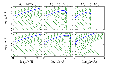
Figure 5.— Mach number versus the radial distance for the winds from a Navarro-Frenk-White dark matter halo. Upper row of plots shows the effect of gravity of dark matter halo only and the lower row takes into account both the gravity due to halo and the effect of AGN. The three plots in each row are for three different halo masses. X-axis in each plot extends upto virial radius corresponding to the halo mass used. The thick blue line represents the solution with a critical point at $R=200$ pc, which is used in this work. We have taken $v_{\star}=180$ km s^-1.

Appendix D Appendix D: Possible effects of radiative cooling

In this section we discuss the effect of radiation loss on the wind properties. So far we have neglected the effect of radiative cooling, since it is known that the energy loss due to radiation is too small to affect the dynamics of winds (Grimes et al. 2009). However the cooling does effect the thermodynamics of the wind and can cause steeper fall in temperature as compared to the case with pure adiabatic expansion. We show this here with a simple case of supersonic escaping wind without gravity for which the wind equation with radiative cooling can be written as,

$$\frac{\mathcal{M}^{2}-1}{\mathcal{M}^{2}(\mathcal{M}^{2}(2/3)+2)}\frac{d\mathcal{M}^{2}}{dr}= {2\over r}+\frac{(\rho^{2}/m_{p}^{2})\Lambda(T)}{2\rho v\ \epsilon(r)}(1+\gamma\mathcal{M}^{2})$$

$$= {2\over r}+\frac{3\dot{M}\Lambda(T)(3+5\mathcal{M}^{2})(3+\mathcal{M}^{2})}{16\pi\ \epsilon(r)^{2}\mathcal{M}^{2}}$$ (D1)

where we have used $\rho=\dot{M}/(4\pi vr^{2})$, $\gamma=5/3$ and $c_{s}^{2}=2\epsilon(r)/(\mathcal{M}^{2}+3)$. Here $\Lambda(T)$ is the cooling rate in erg cm³ s^-1. We use $\Lambda\propto T^{0.8}$ for the temperature range $10^{4}<T<10^{7}$ and $\Lambda\propto T^{2}$ in the temperature range $10^{4}<T<10^{5}$ (Sutherland & Dopita 1993). To solve this equation we have to supply $\epsilon(r)$ and $\dot{M}$. The specific enthalpy, $\epsilon(r)$ can be obtained from the integral of energy equation which is given below,

$$\epsilon(r)={v^{2}\over 2}+{c_{s}^{2}\over\gamma-1}=\frac{\dot{E}}{\dot{M}}-{1\over\dot{M}}\int_{R}^{r}{\rho^{2}\Lambda_{\rm cool}\over m_{p}}(4\pi r^{2})dr=\frac{\dot{E}}{\dot{M}}-{\dot{E}_{cool}(r)\over\dot{M}}$$ (D2)

Considering the fact that total energy extracted by cooling over the entire path is $\sim 10$% of the adiabatic losses (Wang 1995; Grimes et al. 2009) we can neglect $\dot{E}_{cool}$ as compared to $\dot{E}$. Thus we get $\epsilon(r)=\dot{E}/\dot{M}=2v_{\star}^{2}$. Using the $\epsilon(r)$ and a value for $\dot{M}$ in equation D1, we can solve it to obtain Mach number as a function of distance.

In Figure 6 we plot the sound speed $c_{s}=[2\epsilon(r)/(\mathcal{M}^{2}+3)]^{1/2}$ against r, where $\mathcal{M}$ is obtained by solving equation D1. We have solved equation D1 for the quiescent mode ($v_{\star}=180$ km s^-1) and the starburst mode ($v_{\star}=500$ km s^-1). We have used $\dot{M}\sim 1\ {\rm M}_{\odot}$/yr and $10\ {\rm M}_{\odot}$/yr as two fiducial value of mass loss rate for the quiescent mode and the starburst mode respectively. The sound speed corresponding to quiescent mode is shown by dotted line and that of the starburst mode by a dashed line. We have also shown the corresponding cases without cooling using a dash-dotted and a solid line.

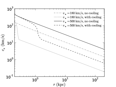
Figure 6.— Sound speed for the wind with cooling is compared with the corresponding case without cooling. The Solid and dash dotted lines represent the case without cooling for quiescent mode and starburst mode respectively. Their counterparts with cooling are shown by dashed and dotted lines.

By comparing the sound speeds with and without cooling, we find that the cooling causes the temperature to decay more rapidly. Also cooling is effective at smaller distances ($r<10$ kpc) as the density and temperature are larger there. Wind speed is given by the relation $\epsilon(r)=v^{2}/2+c_{s}^{2}/(\gamma-1)\sim 2v_{\star}^{2}$. The terminal wind speed is obtained by neglecting the sound speed which is known to decrease with distance. As the sound speed go down even more rapidly in case of cooling, therefore the wind speed beyond a distance of 10 kpc does not differ from the case without cooling and is given by, $v_{\rm wind}\approx 2v_{\star}$. We would like to mention here that qualitatively similar and quantitatively more accurate result has also been obtained by numerically solving the basic fluid equations with cooling for winds from individual star clusters in Silich et al. (2004) and Tenorio-Tagle et al. (2007). Whether the flow undergoing radiative energy losses can achieve a steady state, is also an interesting problem. We refer the reader to Silich et al. (2003) where the time dependent problem on a 2-D grid has been attempted and the result show that the flow can become steady after sufficient amount of time.

Appendix E Appendix E: Coupling between dust and gas

The equation for motion of dust grains acted upon by the radiation from AGN can be written as,

$$v_{\rm dr}{dv_{\rm dr}\over dr}={\pi a^{2}Q_{\rm rp}L\over 4\pi r^{2}c\ m_{d}}-f_{\rm drag}-f_{\rm grav}$$ (E1)

The first term on right hand side is the force of radiation per unit mass in which $Q_{\rm rp}$ is the radiation pressure mean efficiency, $a$ is the size and $m_{d}$ is the mass of the dust grain. $f_{\rm grav}$ is the gravitational force per unit mass and $f_{\rm drag}$ is the drag force per unit mass due to the gas through which the dust grains drift with a velocity $v_{\rm dr}$. This drag force is given by,

$$f_{\rm drag}={\rho\pi a^{2}v^{2}\over m_{d}}$$ (E2)

where $\rho$ and $v$ is the density and velocity of the gas, and $a$ and $m_{d}$ is the size and mass of dust grain respectively. The drag force is a resistive force for the dust but the same drag is a driving force for the gas. One has to simultaneously solve this equation along with the gas momentum equation to work out the general two phase structure of dusty winds. However many essential features can be captured in a so called ’single fluid approximation’ where the dust grains attain a terminal drift speed and then the above written dust momentum equation need not be solved (Simis & Woitke 2004). In that case one can substitute the entire radiation force into the gas momentum equation (Equation 2) because of the exact momentum coupling between dust and gas. The dust grains receive momentum from photons and then pass it on to gas particles via collisions which further distribute it to other gas particles (Gilman 1972).

The momentum coupling and single fluid approximation can be applied if the dust grains attain a terminal drift speed quickly within a short distance once they start moving. We can now verify the validity of momentum coupling in the present case of a galactic outflow. Assuming a typical density profile $\rho=\rho_{o}(r_{o}/r)^{2}$ and neglecting the gravity in comparison to strong forces of radiation and drag, we can integrate equation E1 to obtain the following solution (see also Gilman 1972),

$$v_{\rm dr}^{2}(r)=v_{\rm T}^{2}\left[1-\exp\left(-{2\ell\over r_{o}}(1-r_{o}/r)\right)\right]$$ (E3)

where the terminal drift speed of dust grains is, $v_{\rm T}=[Q_{\rm rp}L/4\pi c\rho_{o}r_{o}^{2}]^{1/2}$ with $l=\rho_{o}r_{o}^{2}\pi a^{2}/m_{d}$ and $r_{o}$ is the launching radius. How quickly the terminal drift speed is achieved, is decided by the value of the multiplicative factor $2l/r_{o}$ in the exponential. We can estimate $\ell$ for a typical grain size of $0.1\ \mu$m, and a grain mass density of $3$ g cm^-3. The quantity $\rho_{o}r_{o}^{2}=\rho_{R}R^{2}$, where $R=200$ pc is the critical point, $\rho_{R}=1$ m_p cm^-3 which is a typical value at the critical point in our wind models. Using these values we get $\ell\approx 5$ kpc. If the dust grains are launched at $r_{o}\sim 10$ pc, we have $2\ell/r_{o}\sim 10^{3}$ and even for $r_{o}=100$ pc we obtain $2\ell/r_{o}\sim 10^{2}$. These large values of $2\ell/r_{o}$ imply that the grains attain drift speed within a short distance. Once the grains are moving with the constant terminal drift speed ($v_{\rm T}$) the entire radiation force is transferred to the gas via the drag force. Therefore the exact coupling between the dust and the gas is justified. Thus the momentum injection force per unit mass of the gas is simply given by $f(r)=n_{d}m_{d}f_{\rm drag}/\rho$. As the dust is moving with a terminal speed, it implies that the drag force is equal to the radiation force. Therefore we can substitute the radiation force in place of $f_{\rm drag}$ to obtain the following expression for force on gas ($f(r)$),

$$f(r)={n_{d}Q_{\rm rp}\pi a^{2}\over\rho}{L\over 4\pi r^{2}c}=\kappa{L\over 4\pi r^{2}c}$$ (E4)

where $\kappa$ is the opacity for a mixture of dust and gas.

References

- Alexander et al. (2010) Alexander, D. M., Swinbank, A. M., Smail, I., McDermid, R., & Nesvadba, N. P. H. 2010, MNRAS, 402, 2211
- Baes et al. (2003) Baes, M., Buyle, P., Hau, G. K. T., & Dejonghe, H. 2003, MNRAS, 341, L44
- Bardeen & Berger (1978) Bardeen, J. M., & Berger, B. K. 1978, ApJ, 221, 105
- Baugh (2006) Baugh, C. M. 2006, Reports on Progress in Physics, 69, 3101
- Behroozi et al. (2010) Behroozi, P. S., Conroy, C., & Wechsler, R. H. 2010, ApJ, 717, 379
- Binney (2004) Binney, J. 2004, MNRAS, 347, 1093
- Binney & Tremaine (2008) Binney, J., & Tremaine, S. 2008, Galactic Dynamics: Second Edition (Princeton University Press)
- Blanton et al. (2008) Blanton, M. R., Geha, M., & West, A. A. 2008, ApJ, 682, 861
- Bouché et al. (2012) Bouché, N., Hohensee, W., Vargas, R., et al. 2012, MNRAS, 3207
- Bower et al. (2006) Bower, R. G., Benson, A. J., Malbon, R., et al. 2006, MNRAS, 370, 645
- Breitschwerdt et al. (1991) Breitschwerdt, D., McKenzie, J. F., & Völk, H. J. 1991, A&A, 245, 79
- Bryan & Norman (1998) Bryan, G. L., & Norman, M. L. 1998, ApJ, 495, 80
- Bullock et al. (2001) Bullock, J. S., Kolatt, T. S., Sigad, Y., et al. 2001, MNRAS, 321, 559
- Burke (1968) Burke, J. A. 1968, MNRAS, 140, 241
- Cattaneo et al. (2006) Cattaneo, A., Dekel, A., Devriendt, J., Guiderdoni, B., & Blaizot, J. 2006, MNRAS, 370, 1651
- Chattopadhyay et al. (2012) Chattopadhyay, I., Sharma, M., Nath, B. B., & Ryu, D. 2012, MNRAS, 423, 2153
- Chevalier & Clegg (1985) Chevalier, R. A., & Clegg, A. W. 1985, Nature, 317, 44
- Conroy et al. (2007) Conroy, C., Prada, F., Newman, J. A., et al. 2007, ApJ, 654, 153
- Cooper et al. (2008) Cooper, J. L., Bicknell, G. V., Sutherland, R. S., & Bland-Hawthorn, J. 2008, ApJ, 674, 157
- Cooper et al. (2009) —. 2009, ApJ, 703, 330
- Croton et al. (2006) Croton, D. J., Springel, V., White, S. D. M., et al. 2006, MNRAS, 365, 11
- Debuhr et al. (2012) Debuhr, J., Quataert, E., & Ma, C.-P. 2012, MNRAS, 420, 2221
- Dekel & Silk (1986) Dekel, A., & Silk, J. 1986, ApJ, 303, 39
- Dekel & Woo (2003) Dekel, A., & Woo, J. 2003, MNRAS, 344, 1131
- Di Matteo et al. (2005) Di Matteo, T., Springel, V., & Hernquist, L. 2005, Nature, 433, 604
- Diamond-Stanic et al. (2012) Diamond-Stanic, A. M., Moustakas, J., Tremonti, C. A., et al. 2012, ApJ, 755, L26
- Dorodnitsyn et al. (2011) Dorodnitsyn, A., Bisnovatyi-Kogan, G. S., & Kallman, T. 2011, ApJ, 741, 29
- Draine (2003) Draine, B. T. 2003, ARA&A, 41, 241
- Dunn et al. (2010) Dunn, J. P., Bautista, M., Arav, N., et al. 2010, ApJ, 709, 611
- Everett & Murray (2007) Everett, J. E., & Murray, N. 2007, ApJ, 656, 93
- Faucher-Giguère & Quataert (2012) Faucher-Giguère, C.-A., & Quataert, E. 2012, MNRAS, 3450
- Ferrarese (2002) Ferrarese, L. 2002, ApJ, 578, 90
- Feruglio et al. (2010) Feruglio, C., Maiolino, R., Piconcelli, E., et al. 2010, A&A, 518, L155
- Fontanot et al. (2009) Fontanot, F., De Lucia, G., Monaco, P., Somerville, R. S., & Santini, P. 2009, MNRAS, 397, 1776
- Fu & Stockton (2009) Fu, H., & Stockton, A. 2009, ApJ, 690, 953
- Gebhardt et al. (2000) Gebhardt, K., Bender, R., Bower, G., et al. 2000, ApJ, 539, L13
- Geha et al. (2006) Geha, M., Blanton, M. R., Masjedi, M., & West, A. A. 2006, ApJ, 653, 240
- Gilman (1972) Gilman, R. C. 1972, ApJ, 178, 423
- Gilmore et al. (2002) Gilmore, G., Wyse, R. F. G., & Norris, J. E. 2002, ApJ, 574, L39
- Granato et al. (2004) Granato, G. L., De Zotti, G., Silva, L., Bressan, A., & Danese, L. 2004, ApJ, 600, 580
- Grimes et al. (2009) Grimes, J. P., Heckman, T., Aloisi, A., et al. 2009, ApJS, 181, 272
- Gültekin et al. (2009) Gültekin, K., Richstone, D. O., Gebhardt, K., et al. 2009, ApJ, 698, 198
- Heckman et al. (1993) Heckman, T. M., Lehnert, M. D., & Armus, L. 1993, in Astrophysics and Space Science Library, Vol. 188, The Environment and Evolution of Galaxies, ed. J. M. Shull & H. A. Thronson, 455
- Heckman et al. (2000) Heckman, T. M., Lehnert, M. D., Strickland, D. K., & Armus, L. 2000, ApJS, 129, 493
- Holzer & Axford (1970) Holzer, T. E., & Axford, W. I. 1970, ARA&A, 8, 31
- Hopkins et al. (2012) Hopkins, P. F., Quataert, E., & Murray, N. 2012, MNRAS, 421, 3522
- Ipavich (1975) Ipavich, F. M. 1975, ApJ, 196, 107
- Johnson & Axford (1971) Johnson, H. E., & Axford, W. I. 1971, ApJ, 165, 381
- Keeney et al. (2006) Keeney, B. A., Danforth, C. W., Stocke, J. T., et al. 2006, ApJ, 646, 951
- King (2003) King, A. 2003, ApJ, 596, L27
- King (2005) —. 2005, ApJ, 635, L121
- King et al. (2011) King, A. R., Zubovas, K., & Power, C. 2011, MNRAS, 415, L6
- Komatsu et al. (2009) Komatsu, E., Dunkley, J., Nolta, M. R., et al. 2009, ApJS, 180, 330
- Kormendy & Bender (2011) Kormendy, J., & Bender, R. 2011, Nature, 469, 377
- Kornei et al. (2012) Kornei, K. A., Shapley, A. E., Martin, C. L., et al. 2012, ArXiv e-prints
- Krolik & Begelman (1988) Krolik, J. H., & Begelman, M. C. 1988, ApJ, 329, 702
- Kurosawa & Proga (2009) Kurosawa, R., & Proga, D. 2009, ApJ, 693, 1929
- Larson (1974) Larson, R. B. 1974, MNRAS, 169, 229
- Leauthaud et al. (2012) Leauthaud, A., Tinker, J., Bundy, K., et al. 2012, ApJ, 744, 159
- Li & Draine (2001) Li, A., & Draine, B. T. 2001, ApJ, 554, 778
- Mandelbaum et al. (2006) Mandelbaum, R., Seljak, U., Kauffmann, G., Hirata, C. M., & Brinkmann, J. 2006, MNRAS, 368, 715
- Marcolini et al. (2005) Marcolini, A., Strickland, D. K., D’Ercole, A., Heckman, T. M., & Hoopes, C. G. 2005, MNRAS, 362, 626
- Martin (1999) Martin, C. L. 1999, ApJ, 513, 156
- Martin (2005) —. 2005, ApJ, 621, 227
- Mathews & Baker (1971) Mathews, W. G., & Baker, J. C. 1971, ApJ, 170, 241
- McQuillin & McLaughlin (2012) McQuillin, R. C., & McLaughlin, D. E. 2012, MNRAS, 423, 2162
- Mo et al. (1998) Mo, H. J., Mao, S., & White, S. D. M. 1998, MNRAS, 295, 319
- More et al. (2011) More, S., van den Bosch, F. C., Cacciato, M., et al. 2011, MNRAS, 410, 210
- Morganti et al. (2007) Morganti, R., Holt, J., Saripalli, L., Oosterloo, T. A., & Tadhunter, C. N. 2007, A&A, 476, 735
- Moster et al. (2010) Moster, B. P., Somerville, R. S., Maulbetsch, C., et al. 2010, ApJ, 710, 903
- Muñoz-Cuartas et al. (2011) Muñoz-Cuartas, J. C., Macciò, A. V., Gottlöber, S., & Dutton, A. A. 2011, MNRAS, 411, 584
- Murray et al. (1995) Murray, N., Chiang, J., Grossman, S. A., & Voit, G. M. 1995, ApJ, 451, 498
- Murray et al. (2011) Murray, N., Ménard, B., & Thompson, T. A. 2011, ApJ, 735, 66
- Murray et al. (2005) Murray, N., Quataert, E., & Thompson, T. A. 2005, ApJ, 618, 569
- Nath & Silk (2009) Nath, B. B., & Silk, J. 2009, MNRAS, 396, L90
- Navarro et al. (1996) Navarro, J. F., Frenk, C. S., & White, S. D. M. 1996, ApJ, 462, 563
- Novak et al. (2012) Novak, G. S., Ostriker, J. P., & Ciotti, L. 2012, ArXiv e-prints: 1203.6062
- Oppenheimer & Davé (2006) Oppenheimer, B. D., & Davé, R. 2006, MNRAS, 373, 1265
- Parker (1965) Parker, E. N. 1965, Space Sci. Rev., 4, 666
- Pizagno et al. (2007) Pizagno, J., Prada, F., Weinberg, D. H., et al. 2007, AJ, 134, 945
- Pizzella et al. (2005) Pizzella, A., Corsini, E. M., Dalla Bontà, E., et al. 2005, ApJ, 631, 785
- Proga et al. (2000) Proga, D., Stone, J. M., & Kallman, T. R. 2000, ApJ, 543, 686
- Puchwein & Springel (2012) Puchwein, E., & Springel, V. 2012, ArXiv e-prints: 1205.2694
- Risaliti & Elvis (2010) Risaliti, G., & Elvis, M. 2010, A&A, 516, A89
- Rupke et al. (2005a) Rupke, D. S., Veilleux, S., & Sanders, D. B. 2005a, ApJ, 632, 751
- Rupke et al. (2005b) —. 2005b, ApJS, 160, 115
- Rupke & Veilleux (2011) Rupke, D. S. N., & Veilleux, S. 2011, ApJ, 729, L27
- Samui et al. (2008) Samui, S., Subramanian, K., & Srianand, R. 2008, MNRAS, 385, 783
- Schwartz et al. (2006) Schwartz, C. M., Martin, C. L., Chandar, R., et al. 2006, ApJ, 646, 858
- Shankar et al. (2006) Shankar, F., Lapi, A., Salucci, P., De Zotti, G., & Danese, L. 2006, ApJ, 643, 14
- Sharma & Nath (2012) Sharma, M., & Nath, B. B. 2012, ApJ, 750, 55
- Sharma et al. (2011) Sharma, M., Nath, B. B., & Shchekinov, Y. 2011, ApJ, 736, L27
- Silich et al. (2011) Silich, S., Bisnovatyi-Kogan, G., Tenorio-Tagle, G., & Martínez-González, S. 2011, ApJ, 743, 120
- Silich et al. (2003) Silich, S., Tenorio-Tagle, G., & Muñoz-Tuñón, C. 2003, ApJ, 590, 791
- Silich et al. (2004) Silich, S., Tenorio-Tagle, G., & Rodríguez-González, A. 2004, ApJ, 610, 226
- Silk & Nusser (2010) Silk, J., & Nusser, A. 2010, ApJ, 725, 556
- Silk & Rees (1998) Silk, J., & Rees, M. J. 1998, A&A, 331, L1
- Simis & Woitke (2004) Simis, Y., & Woitke, P. 2004, in Asymptotic giant branch stars, ed. H. J. Habing & H. Olofsson, Astronomy and Astrophysics Library, Springer, 291
- Somerville et al. (2008) Somerville, R. S., Hopkins, P. F., Cox, T. J., Robertson, B. E., & Hernquist, L. 2008, MNRAS, 391, 481
- Somerville et al. (2004) Somerville, R. S., Moustakas, L. A., Mobasher, B., et al. 2004, ApJ, 600, L135
- Springel et al. (2005) Springel, V., Di Matteo, T., & Hernquist, L. 2005, ApJ, 620, L79
- Springob et al. (2005) Springob, C. M., Haynes, M. P., Giovanelli, R., & Kent, B. R. 2005, ApJS, 160, 149
- Stinson et al. (2012) Stinson, G. S., Brook, C., Prochaska, J. X., et al. 2012, MNRAS, 3506
- Strickland & Heckman (2009) Strickland, D. K., & Heckman, T. M. 2009, ApJ, 697, 2030
- Strickland et al. (2004) Strickland, D. K., Heckman, T. M., Colbert, E. J. M., Hoopes, C. G., & Weaver, K. A. 2004, ApJ, 606, 829
- Strickland & Stevens (2000) Strickland, D. K., & Stevens, I. R. 2000, MNRAS, 314, 511
- Sturm et al. (2011) Sturm, E., González-Alfonso, E., Veilleux, S., et al. 2011, ApJ, 733, L16
- Suchkov et al. (1994) Suchkov, A. A., Balsara, D. S., Heckman, T. M., & Leitherer, C. 1994, ApJ, 430, 511
- Sutherland & Dopita (1993) Sutherland, R. S., & Dopita, M. A. 1993, ApJS, 88, 253
- Tenorio-Tagle et al. (2007) Tenorio-Tagle, G., Wünsch, R., Silich, S., & Palouš, J. 2007, ApJ, 658, 1196
- Tremaine et al. (2002) Tremaine, S., Gebhardt, K., Bender, R., et al. 2002, ApJ, 574, 740
- Tremonti et al. (2007) Tremonti, C. A., Moustakas, J., & Diamond-Stanic, A. M. 2007, ApJ, 663, L77
- Trump et al. (2006) Trump, J. R., Hall, P. B., Reichard, T. A., et al. 2006, ApJS, 165, 1
- Tumlinson et al. (2011) Tumlinson, J., Thom, C., Werk, J. K., et al. 2011, Science, 334, 948
- Uhlig et al. (2012) Uhlig, M., Pfrommer, C., Sharma, M., et al. 2012, MNRAS, 423, 2374
- van de Voort & Schaye (2012) van de Voort, F., & Schaye, J. 2012, ArXiv e-prints: 1207.5512
- Veilleux et al. (2005) Veilleux, S., Cecil, G., & Bland-Hawthorn, J. 2005, ARA&A, 43, 769
- Villar-Martín et al. (2011) Villar-Martín, M., Humphrey, A., Delgado, R. G., Colina, L., & Arribas, S. 2011, MNRAS, 418, 2032
- Volonteri & Stark (2011) Volonteri, M., & Stark, D. P. 2011, MNRAS, 417, 2085
- Wang (1995) Wang, B. 1995, ApJ, 444, 590
- Westmoquette et al. (2012) Westmoquette, M. S., Clements, D. L., Bendo, G. J., & Khan, S. A. 2012, MNRAS, 424, 416
- Wünsch et al. (2011) Wünsch, R., Silich, S., Palouš, J., Tenorio-Tagle, G., & Muñoz-Tuñón, C. 2011, ApJ, 740, 75
- Wyithe & Loeb (2003) Wyithe, J. S. B., & Loeb, A. 2003, ApJ, 595, 614