Polarized line formation with $J$-state interference in the presence of magnetic fields: A heuristic treatment of collisional frequency redistribution

Abstract

An expression for the partial frequency redistribution (PRD) matrix for line scattering in a two-term atom, which includes the $J$-state interference between its fine structure line components is derived. The influence of collisions (both elastic and inelastic) and an external magnetic field on the scattering process is taken into account. The lower term is assumed to be unpolarized and infinitely sharp. The linear Zeeman regime in which the Zeeman splitting is much smaller than the fine structure splitting is considered. The inelastic collision rates between the different levels are included in our treatment. We account for the depolarization caused by the collisions coupling the fine structure states of the upper term, but neglect the polarization transfer between the fine structure states. When the fine structure splitting goes to zero, we recover the redistribution matrix that represents the scattering on a two-level atom (which exhibits only $m$-state interference — namely the Hanle effect). The way in which the multipolar index of the scattering atom enters into the expression for the redistribution matrix through the collisional branching ratios is discussed. The properties of the redistribution matrix are explored for a single scattering process for an $L=0\to 1\to 0$ scattering transition with $S=1/2$ (a hypothetical doublet centered at 5000 Å and 5001 Å). Further, a method for solving the Hanle radiative transfer equation for a two-term atom in the presence of collisions, PRD, and $J$-state interference is developed. The Stokes profiles emerging from an isothermal constant property medium are computed.

1 Introduction

The Solar spectrum is linearly polarized due to coherent scattering processes in the Sun’s atmosphere. This linearly polarized spectrum is as rich in spectral structures as the ordinary intensity spectrum, but it differs in appearance and information contents (see Stenflo & Keller [1, 2], Stenflo et al. [3]). It is therefore referred to as the “Second Solar Spectrum”. A weak magnetic field modifies this spectrum through the process of the Hanle effect. This makes the Second Solar Spectrum sensitive to a field strength regime that is inaccessible to the ordinary Zeeman effect. It therefore has the potential to significantly advance our understanding of the Sun’s magnetism. In order to interpret the wealth of information imprinted in the Second Solar Spectrum, it is necessary to develop adequate theoretical tools that can later be used for the polarized line formation calculations.

Stenflo [4, 5] (hereafter S94 and S98 respectively) developed a classical theory for frequency-coherent scattering of polarized radiation in the presence of magnetic fields of arbitrary strength and orientation. This theory was generalized by Bommier & Stenflo [6] (hereafter BS99) to include the effects of partial frequency redistribution (PRD) in the scattering process. Their formulation was restricted to the rest frame of the atom. The transformation to the laboratory frame was presented in Sampoorna et al. [7] (hereafter HZ1) for the special case of a $J=0\to 1\to 0$ scattering transition. Recently Sampoorna [8] has generalized the classical PRD theory of BS99 to treat other types of atomic transitions with arbitrary $J$-quantum numbers.

In Smitha et al. [9] (hereafter P1) we derived the polarized PRD matrices for a two-term atom with an arbitrary $L_{a}\to L_{b}\to L_{a}$ scattering transition, taking into account the effects of $J$-state interference between the fine structure components of the split upper term $L_{b}$ (see Figure 1). However, these expressions were limited to the collisionless regime. In the present paper we generalize the semi-classical theory of Sampoorna [8] to include $J$-state interference for a two-term atom in the presence of collisions. In Smitha et al. [10] (hereafter P3), a simpler version of this theory (see Section 3.2) has already been applied to model the non-magnetic linear polarization observations of $J$-state interference phenomena in the Cr i triplet.

Figure 1: Schematic Level diagram of a two-term atom. The lower term is assumed to be infinitely sharp whereas the upper term is both radiatively and collisionally broadened.

Collisions play a vital role in determining the polarization properties of the scattered radiation. For the case of a two-level atom with unpolarized lower level, Omont et al. [11] developed the quantum theory of polarized scattering in a non-magnetic medium, including PRD effects. They describe in detail the role played by elastic and inelastic collisions. The effects of magnetic fields were considered in Omont et al. [12]. An explicit form of the polarized PRD matrix for resonance scattering on a two-level atom was derived by Domke & Hubeny [13], based on the work of Omont et al. [11], assuming that the lower level is unpolarized. Under the same assumption, a more elegant form of the PRD matrix for both the non-magnetic and magnetic cases was derived in pioneering papers by Bommier [14, 15, 16] using the master equation theory. The equivalence between the QED theory of Bommier [15] and the semi-classical theory was demonstrated in Sampoorna et al. [18] (hereafter HZ2) for a $J=0\to 1\to 0$ scattering transition, and in Sampoorna [8] for an arbitrary $J_{a}\to J_{b}\to J_{a}$ scattering transition. An alternative PRD theory based on the concept of metalevels has been developed by Landi Degl’Innocenti et al. [17] for the collisionless case. This formulation can also deal with $J$-state interference in the presence of magnetic fields.

In the present paper, starting from the Kramers-Heisenberg formula, we derive the expressions for the collisional PRD matrices including the effects of $J$-state interference for a two-term atom. The following assumptions are made:

1. Infinitely sharp lower term.

2. Unpolarized lower term.

3. Weak radiation field limit (i.e., stimulated emission is neglected in comparison with the spontaneous emission).

4. Hyperfine structure is neglected.

5. The effects of inelastic collisions that couple the fine structure states are treated approximately (see below).

6. The depolarizing elastic collisions that couple $m$-states belonging to a given fine structure state $J_{b}$ are taken into account, but are assumed to be independent of the $J$-quantum number for the sake of mathematical simplicity.

7. We restrict our attention to the linear Zeeman regime of magnetic field strengths.

The assumption of an unpolarized lower term is made for the sake of mathematical simplicity, but can often be justified when the lower term represents the ground state of the atom. In the stellar atmospheric conditions the ground state is generally two orders of magnitude more long lived than the excited state, which makes it correspondingly much harder for any ground state polarization to survive collisional and magnetic depolarization, as compared with the excited states (see Kerkeni & Bommier [19]). We also ignore the induced emission, because in scattering problems it acts as a negative absorption and only affects the radiation in the exact forward direction (scattering angle exactly zero). The induced emission probability is nearly three orders of magnitude smaller than the spontaneous emission probability (see Kerkeni & Bommier [19]).

The inelastic collisions between the upper and lower terms are treated exactly while the inelastic collisions between the upper fine structure states are treated approximately. The inelastic collisions between the upper fine structure states (denoted by $\Gamma_{IJ_{b}J_{b^{\prime}}}$) manifest themselves in two different ways, (i) through a depolarization of state $J_{b}$ and (ii) through a transfer of alignment and orientation between $J_{b}$ and $J_{b^{\prime}}$.

Since the colliding particles are isotropically distributed around the radiating atom, they destroy the alignment and thereby depolarize the levels. Therefore the inelastic collisions that take the atom away from the state $J_{b}$ always depolarize $J_{b}$. They also contribute to the inverse lifetime of $J_{b}$ under consideration. In this paper we take into account such inelastic collisions between the fine structure states $J_{b}$ and $J_{b^{\prime}}$ by adding these inelastic collision rates $(\Gamma_{IJ_{b}J_{b^{\prime}}})$ to the inelastic collision rate $\Gamma_{IJ_{b}J_{f}}$ (where $f$ is the final state). The depolarizing effects of these inelastic collisions are similar to the depolarizing effects of elastic collisions. Thus we merge these two effects and define a common damping rate $\gamma_{b}$ for the $J_{b}$ state.

The inelastic collisions between polarized fine structure states can lead to a transfer of alignment and orientation between them (hereafter referred to as the transfer of polarization). This is similar to optical pumping by radiative transitions. The only difference is that the radiative transitions between the fine structure states $J_{b}$ and $J_{b^{\prime}}$ are not allowed. Taking account of such transfer rates caused by inelastic collisions actually involves formulating the statistical equilibrium equations for the concerned states including the atomic polarization of the various states. This is outside the scope of our present paper. A formulation of statistical equilibrium equation including these collisions but neglecting the redistribution effects in scattering has been presented in Kerkeni [20] and Kerkeni & Bommier [19]. They derive the expressions to calculate these rates taking examples of few atomic systems of relevance to the analysis of the second solar spectrum. Our present treatment of inelastic collisions is basically heuristic and only takes into account the depolarizing effects of $\Gamma_{IJ_{b}J_{b^{\prime}}}$.

The frequency redistribution function that describes the effect of collisions in unpolarized radiative transfer is the well known type-III (or $R^{\rm III}$) function of Hummer [21]. Here we describe the matrix generalizations of this standard collisional redistribution function, brought about by the magnetic fields and the $J$-state interference. Using the method described in Appendix C of HZ2, we rewrite the PRD matrices in terms of the irreducible spherical tensors for polarimetry. We discuss in detail the procedure to identify the multipolar index $K$, which needs to be assigned to the branching ratios that govern the effect of the depolarizing collisions. We illustrate the effects of collisions on the Stokes $(I,Q/I,U/I,V/I)$ profiles of the scattered radiation for the 90° single scattering case. Then we present the technique of incorporating this Hanle redistribution matrix for the two-term atom into the polarized radiative transfer equation, and solve it for an isothermal constant property atmospheric slab. In the collisionless case, the relevant redistribution matrix derived in P1 was incorporated into the transfer equation in Smitha et al. [22] (hereafter P2) and solved for a constant property isothermal media in the absence of a magnetic field. The same method of solution presented in P2 is also used here, but including the collisional redistribution in the presence of a magnetic field.

In Section 2 we derive the elements of the ensemble averaged coherency matrix both in the atomic and laboratory frames for a $L_{a}\to L_{b}\to L_{a}$ scattering transition taking into account the elastic collisions. In Section 3 we express the type-III redistribution matrix in terms of the irreducible spherical tensors both for the non-magnetic and magnetic cases. The important question of identifying the multipolar index $K$ that describes the transfer of angular momentum in a scattering event affected by the depolarizing collisions is discussed in detail. The laboratory frame expression for the collisional redistribution matrix is also derived in this section. The procedure to incorporate this redistribution matrix into the polarized radiative transfer equation for both the magnetic and non-magnetic cases is discussed in Section 4. The Stokes profiles resulting from a single $90^{\circ}$ scattering event and from multiple scattering in an isothermal atmospheric slab are presented in Section 5. Concluding remarks are given in Section 6. Finally, in Appendix A we give the expressions for the magnetic redistribution functions of type-III.

2 An approximate treatment of collisions including the $J$-state interference

2.1 A semi-classical formulation for the polarized PRD matrix

The Mueller matrix ${\bf M}$ that describes the transformation from the incident to the scattered Stokes vector is given by

$${\bf M}={\bf T}{\bf W}{\bf T}^{-1},$$ (1)

where ${\bf T}$ and ${\bf T}^{-1}$ are purely mathematical transformation matrices. Their explicit forms are given in Equation (9) of S98. The ${\bf W}$-matrix is defined in Equation (7) of P1. The elements of this matrix contain the bilinear products of the complex probability amplitude $w_{\alpha\beta}(J_{f}\mu_{f}J_{a}\mu_{a})$. These amplitudes for transition from an initial state $a$ to final state $f$ via all intermediate states $b$ are given by the Kramers-Heisenberg formula (see S98 and Sampoorna [8] for historical accounts) as

$$w_{\alpha\beta}\sim\sum_{b}\frac{\left\langle f|{\bf{r\ .\ e_{\alpha}}}|b\right\rangle\left\langle b|{\bf{r\ .\ e_{\beta}}}|a\right\rangle}{\omega_{bf}-\omega-{\rm i}\gamma_{b}/2},$$ (2)

where $\omega=2\pi\xi$ is the angular frequency of the scattered radiation in the atomic rest frame, $\hbar\omega_{bf}$ is the energy difference between the excited and final states, and $\gamma_{b}$ is the damping constant that accounts for the broadening of the excited state $b$, while the initial and the final states are assumed to be infinitely sharp. The damping parameter is assumed to be the same for all the magnetic substates of the excited state. The matrix elements appearing in Equation (2) can be expanded using the Wigner-Eckart theorem as

$$w_{\alpha\beta}(J_{f}\mu_{f}J_{a}\mu_{a})\sim\sum_{J_{b}\mu_{b}}(-1)^{q-q^{\prime}}\sqrt{(2J_{a}+1)(2J_{f}+1)}(2J_{b}+1)(2L_{a}+1)\left\{\begin{array}[]{ccc}L_{a}&L_{b}&1\\ J_{b}&J_{f}&S\\ \end{array}\right\}$$ (5)

$$\times\left\{\begin{array}[]{ccc}L_{a}&L_{b}&1\\ J_{b}&J_{a}&S\\ \end{array}\right\}\left(\begin{array}[]{ccc}J_{b}&J_{a}&1\\ -\mu_{b}&\mu_{a}&-q^{\prime}\\ \end{array}\right)\left(\begin{array}[]{ccc}J_{b}&J_{f}&1\\ -\mu_{b}&\mu_{f}&-q\\ \end{array}\right)\Phi_{\gamma_{b}}(\nu_{J_{b}\mu_{b}J_{f}\mu_{f}}-\xi)\varepsilon^{\alpha\ast}_{q}\varepsilon^{\beta}_{q^{\prime}},$$ (12)

where $\mu_{b}$ represents the magnetic substates of the upper state $b$ with total angular momentum quantum number $J_{b}$, orbital angular momentum quantum number $L_{b}$, and spin $S$. The quantities $J_{a}$ and $J_{f}$ are respectively the total angular momentum quantum numbers of the initial and final states $a$ and $f$ with orbital angular momentum quantum number $L_{a}$, and magnetic substates $\mu_{a}$ and $\mu_{f}$. The quantities $\varepsilon$ are the geometrical factors (see Equations (2) and (27) of S98), with $\alpha$ and $\beta$ denoting the outgoing and incoming radiation, respectively. In Equation (12), $q=\mu_{f}-\mu_{b}$ and $q^{\prime}=\mu_{a}-\mu_{b}$. In the rest of the paper we denote the indices as follows for the sake of convenience

$$J_{b}=b,\ J_{a}=a,\ J_{f}=f;\quad J_{b}\mu_{b}=b_{m},\ J_{a}\mu_{a}=a_{m},\ J_{f}\mu_{f}=f_{m},$$

$$\ \ \ \ \ \ \ \ \ \ \ \ \ \ J_{b^{\prime}}\mu_{b^{\prime}}=b^{\prime}_{m},\ J_{b}\mu_{b^{\prime\prime}}=b^{\prime\prime}_{m},\ J_{b^{\prime}}\mu_{b^{\prime\prime\prime}}=b^{\prime\prime\prime}_{m}.$$ (13)

The frequency-normalized profile function is given by

$$\Phi_{\gamma_{b}}(\nu_{b_{m}f_{m}}-\xi)=\frac{1/(\pi\rm{i})}{\nu_{b_{m}f_{m}}-\xi-{\rm i}\gamma_{b}/(4\pi)}\ \ {\rm{with}}\ \ \ \nu_{b_{m}f_{m}}=\nu_{bf}+(g_{b}\mu_{b}-g_{f}\mu_{f})\nu_{L}.$$ (14)

Here $h\nu_{bf}$ is the energy difference between the upper ($J_{b}$) and lower ($J_{f}$) states in the absence of magnetic fields, $g_{b}$, $g_{f}$ are the Landé factors of these states, and $\nu_{L}$ is the Larmor frequency. Equation (12) refers to the case of frequency-coherent scattering in the atomic rest frame.

The phenomenological extension of Equation (12) to the case of PRD is achieved by treating each radiative emission transition between magnetic substates $\mu_{b}$ and $\mu_{f}$ in terms of a damped oscillator that is truncated by collisions (see HZ1). In other words, in Equation (12) we make the following replacement for the profile function :

$$\Phi_{\gamma_{b}}(\nu_{b_{m}f_{m}}-\xi)\longrightarrow(\tilde{r}_{b_{m}})_{a_{m}f_{m}},$$ (15)

where the Fourier-transformed solution of the time-dependent oscillator equation is given by (see BS99)

$$(\tilde{r}_{b_{m}})_{a_{m}f_{m}}=(\tilde{r}^{\rm stat}_{b_{m}})_{a_{m}f_{m}}+\ C\ (\tilde{r}^{\rm trans}_{b_{m}})_{a_{m}f_{m}}.$$ (16)

Here we have omitted the unimportant phase factor, as it vanishes in the bilinear product
$(\tilde{r}_{b_{m}})_{a_{m}f_{m}}(\tilde{r}^{\ast}_{{b^{\prime}}_{m}})_{a_{m}f_{m}}$. The constant $C$ in Equation (16) defines the relative amplitudes of the stationary and the transitory parts of the solution, which are given by

$$(\tilde{r}^{\rm stat}_{b_{m}})_{a_{m}f_{m}}=\Phi_{\gamma_{b}}(\nu_{b_{m}a_{m}}-\xi^{\prime})\delta(\xi-\xi^{\prime}-\nu_{a_{m}f_{m}}),$$ (17)

$$(\tilde{r}^{\rm trans}_{b_{m}})_{a_{m}f_{m}}=\Phi_{\gamma_{b}}(\nu_{b_{m}a_{m}}-\xi^{\prime})\Phi_{\gamma_{b}}(\nu_{b_{m}f_{m}}-\xi)\left[1-{\rm e}^{-{\rm i}(\omega_{b_{m}f_{m}}-{\rm i}\gamma_{b}/2-\omega)t_{c}}\right].$$ (18)

Here $\xi^{\prime}$ denotes the frequency of the incoming photon in the atomic rest frame, $t_{c}$ is the time between two successive collisions, $\omega_{b_{m}f_{m}}=2\pi\nu_{b_{m}f_{m}}$. The profile function $\Phi_{\gamma_{b}}(\nu_{b_{m}a_{m}}-\xi^{\prime})$ is given by Equation (14) with $\xi$ replaced by $\xi^{\prime}$, while $\nu_{b_{m}f_{m}}$ is replaced by $\nu_{b_{m}a_{m}}$ that is defined similar to Equation (14). In Equation (17), $\nu_{a_{m}f_{m}}$ appearing in the delta function is demanded by energy conservation (see Equation (9.10) of S94), and is given by

$$\nu_{a_{m}f_{m}}=\nu_{af}+(g_{a}\mu_{a}-g_{f}\mu_{f})\nu_{L},$$ (19)

where $h\nu_{af}$ is the energy difference between the states $J_{a}$ and $J_{f}$ in the absence of a magnetic field.

2.2 Coherency matrix in the atomic rest frame

The elements of the ensemble averaged coherency matrix $\langle\tilde{r}_{b_{m}}\tilde{r}^{\ast}_{{b^{\prime}}_{m}}\rangle_{a_{m}f_{m}}$ can be derived starting from Equations (17) and (18), applying the same steps that are described in detail in BS99. These elements are contained in the bilinear product $w_{\alpha\beta}(f_{m}a_{m})w^{\ast}_{\alpha^{\prime}\beta^{\prime}}(f_{m}a_{m})$. In the atomic rest frame ensemble averaged coherency matrix elements are given by

$$\langle\tilde{r}_{b_{m}}\tilde{r}^{\ast}_{{b^{\prime}}_{m}}\rangle_{a_{m}f_{m}}=A_{b{b^{\prime}}}\cos\beta_{{b^{\prime}}_{m}b_{m}}\ {\rm e}^{{\rm i}\beta_{{b^{\prime}}_{m}b_{m}}}\ \Phi^{{{\gamma}_{bb^{\prime}}+\gamma_{c}}}_{b_{m}{b^{\prime}}_{m}a_{m}}(\xi^{\prime})\delta(\xi-\xi^{\prime}-\nu_{a_{m}f_{m}})$$

$$+B_{b{b^{\prime}}}\cos\beta_{{b^{\prime}}_{m}b_{m}}\cos\alpha_{{b^{\prime}}_{m}b_{m}}{\rm e}^{{\rm i}(\beta_{{b^{\prime}}_{m}b_{m}}+\alpha_{{b^{\prime}}_{m}b_{m}})}\Phi^{{{\gamma}}_{bb^{\prime}}+\gamma_{c}}_{b_{m}{b^{\prime}}_{m}a_{m}}(\xi^{\prime})\Phi^{{{\gamma}}_{bb^{\prime}}+\gamma_{c}}_{b_{m}{b^{\prime}}_{m}f_{m}}(\xi),$$ (20)

where the angles $\beta_{{b^{\prime}}_{m}b_{m}}$ and $\alpha_{{b^{\prime}}_{m}b_{m}}$ (arising due to the combined effects of the $J$-state and $m$-state interferences) are defined respectively by

$$\tan\beta_{{b^{\prime}}_{m}b_{m}}={\omega_{{b^{\prime}}b}+(g_{b^{\prime}}\mu_{b^{\prime}}-g_{b}\mu_{b})\omega_{L}\over{{\gamma}_{{b^{\prime}}b}+\gamma_{c}}};\quad\tan\alpha_{{b^{\prime}}_{m}b_{m}}={\omega_{{b^{\prime}}b}+(g_{b^{\prime}}\mu_{b^{\prime}}-g_{b}\mu_{b})\omega_{L}\over{{\gamma}_{{b^{\prime}}b}+\gamma_{c}/2}},$$ (21)

with ${\gamma}_{bb^{\prime}}$ given by

$${\gamma}_{b{b^{\prime}}}=\frac{\gamma_{b}+\gamma_{{b^{\prime}}}}{2}={\gamma}_{{b^{\prime}}b}.$$ (22)

Here $\gamma_{c}$ is the collisional damping constant, while $\hbar\omega_{{b^{\prime}}b}$ is the energy difference between the $J_{b^{\prime}}$ and $J_{b}$ states in the absence of a magnetic field. The elastic collisional rates are in general different for each fine structure component ($J_{b}$) of the upper term. However, for simplicity we assume them to be independent of the $J$-quantum numbers.

$A_{b{b^{\prime}}}$ and $B_{b{b^{\prime}}}$ are the branching ratios for a two-term atom. The explicit expressions for them will be defined later in Section 3.1.

Like in P1, we limit the treatment to the linear Zeeman regime, in which the Zeeman splitting is much smaller than the fine structure splitting. When $J_{b}\neq J_{b^{\prime}}$ the contributions from the second terms with $\omega_{L}$ in Equation (21) to the angles $\beta_{{b^{\prime}}_{m}b_{m}}$ and $\alpha_{{b^{\prime}}_{m}b_{m}}$ can therefore be ignored, because they are insignificant in comparison with the first terms. The classical generalized profile function is defined as

$$\Phi^{{\gamma}_{bb^{\prime}}}_{b_{m}{b^{\prime}}_{m}f_{m}}(\xi)={1\over 2}\left[\Phi_{\gamma_{b}}(\nu_{b_{m}f_{m}}-\xi)+\Phi^{\ast}_{\gamma_{b^{\prime}}}(\nu_{{b^{\prime}}_{m}f_{m}}-\xi)\right],$$ (23)

in the same way as in BS99.

2.3 Coherency matrix in the laboratory frame for type-III redistribution

We transform Equation (20) to the laboratory frame using the same steps as described in Section 2.2 of HZ2. Thus the ensemble averaged coherency matrix in the laboratory frame is given by

$$\!\!\!\!\!\!\!\!\langle\tilde{r}_{b_{m}}\tilde{r}^{\ast}_{{b^{\prime}}_{m}}\rangle_{a_{m}f_{m}}=A_{b{b^{\prime}}}\cos\beta_{{b^{\prime}}_{m}b_{m}}{\rm e}^{{\rm i}\beta_{{b^{\prime}}_{m}b_{m}}}\Big{[}(h^{\rm II}_{b_{m},{b^{\prime}}_{m}})_{a_{m}f_{m}}+{\rm i}(f^{\rm II}_{b_{m},{b^{\prime}}_{m}})_{a_{m}f_{m}}\Big{]}\$$

$$+B_{b{b^{\prime}}}\cos\beta_{{b^{\prime}}_{m}b_{m}}\cos\alpha_{{b^{\prime}}_{m}b_{m}}{\rm e}^{{\rm i}(\beta_{{b^{\prime}}_{m}b_{m}}+\alpha_{{b^{\prime}}_{m}b_{m}})}\Big{[}h^{\rm III}_{b_{m}a_{m},{b^{\prime}}_{m}f_{m}}+{\rm i}f^{\rm III}_{b_{m}a_{m},{b^{\prime}}_{m}f_{m}}\Big{]}.$$ (24)

The various auxiliary quantities for type-II redistribution are defined in Section 3 of P1. Hence we do not repeat them here. Hereafter we confine our attention to the collisional redistribution (type-III). The corresponding derivation for pure radiative (collisionless) redistribution (type-II) are given in P1. The auxiliary quantities for type-III redistribution that appear in Equation (24) are defined by

$$h^{\rm III}_{b_{m}a_{m},{b^{\prime}}_{m}f_{m}} = {\frac{1}{4}}\,\Bigg{[}R^{\rm III,\,HH}_{{b^{\prime}}_{m}a_{m},{b^{\prime}}_{m}f_{m}}+R^{\rm III,\,HH}_{{b^{\prime}}_{m}a_{m},b_{m}f_{m}}+R^{\rm III,\,HH}_{b_{m}a_{m},{b^{\prime}}_{m}f_{m}}+R^{\rm III,\,HH}_{b_{m}a_{m},b_{m}f_{m}}\Bigg{]}$$ (25)

$$+{\frac{\rm i}{4}}\,\Bigg{[}R^{\rm III,\,FH}_{{b^{\prime}}_{m}a_{m},{b^{\prime}}_{m}f_{m}}+R^{\rm III,\,FH}_{{b^{\prime}}_{m}a_{m},b_{m}f_{m}}-R^{\rm III,\,FH}_{b_{m}a_{m},{b^{\prime}}_{m}f_{m}}-R^{\rm III,\,FH}_{b_{m}a_{m},b_{m}f_{m}}\Bigg{]}.$$

Similarly we have

$$f^{\rm III}_{b_{m}a_{m},{b^{\prime}}_{m}f_{m}} = {\frac{1}{4}}\,\Bigg{[}R^{\rm III,\,HF}_{{b^{\prime}}_{m}a_{m},{b^{\prime}}_{m}f_{m}}-R^{\rm III,\,HF}_{{b^{\prime}}_{m}a_{m},b_{m}f_{m}}+R^{\rm III,\,HF}_{b_{m}a_{m},{b^{\prime}}_{m}f_{m}}-R^{\rm III,\,HF}_{b_{m}a_{m},b_{m}f_{m}}\Bigg{]}$$ (26)

$$+{\frac{\rm i}{4}}\,\Bigg{[}R^{\rm III,\,FF}_{{b^{\prime}}_{m}a_{m},{b^{\prime}}_{m}f_{m}}-R^{\rm III,\,FF}_{{b^{\prime}}_{m}a_{m},b_{m}f_{m}}-R^{\rm III,\,FF}_{b_{m}a_{m},{b^{\prime}}_{m}f_{m}}+R^{\rm III,\,FF}_{b_{m}a_{m},b_{m}f_{m}}\Bigg{]}.$$

The magnetic redistribution functions of type-III appearing in the above equations are defined in A.

3 The PRD matrix expressed in terms of irreducible tensors

The importance of expressing the PRD matrices in terms of the irreducible spherical tensors introduced by Landi Degl’Innocenti [30] has been discussed in P1. The definition and properties of irreducible spherical tensors are described in detail in Landi Degl’Innocenti & Landolfi [23] (hereafter LL04). The way to incorporate these tensors in the analytic form of the PRD matrix derived from a semi-classical approach has been described in HZ2 (see also Section 4 of P1). Applying the same method we have obtained an expression for the type-III redistribution matrix in terms of irreducible spherical tensors. The case of the type-II redistribution matrix has been discussed in Section 4 of P1.

As in P1 we now express the type-III PRD matrix derived in Section 2 in terms of ${\mathcal{T}}^{K}_{Q}(i,{\bm{n}})$, where $i=0,1,2,3$, and $K=0,1,2$ with $-K\leq Q\leq+K$. Following the same procedure as discussed in Section 4 of P1, the matrix $T^{\rm S}_{\mu\nu,\rho\sigma}$ of Equation (22) in P1, which describes the transformation of the elements of the coherency matrix, can be written in the atomic rest frame as

$$\!\!\!\!\!\!\!\!\!T^{\rm S}_{\mu\nu,\rho\sigma}(\xi,{\bm{n}};\xi^{\prime},{\bm{n}}^{\prime},{\bm{B}})=(2L_{a}+1)^{2}\sum_{a_{m}f_{m}b_{m}{b^{\prime}}_{m}}G\ Z_{6}Z_{3}\ \ (-1)^{q-q^{\prime}+q^{\prime\prime}-q^{\prime\prime\prime}}{\mathcal{E}}^{\rm S}_{qq^{\prime\prime}}(\mu,\nu,{\bm{n}}){\mathcal{E}}^{\rm S}_{q^{\prime\prime\prime}q^{\prime}}(\sigma,\rho,{\bm{n}}^{\prime})$$

$$\times\Big{\{}A_{b{b^{\prime}}}\cos\beta_{{b^{\prime}}_{m}b_{m}}\ {\rm e}^{{\rm i}\beta_{{b^{\prime}}_{m}b_{m}}}\ \Phi^{{{\gamma}_{bb^{\prime}}+\gamma_{c}}}_{b_{m}{b^{\prime}}_{m}a_{m}}(\xi^{\prime})\delta(\xi-\xi^{\prime}-\nu_{a_{m}f_{m}})$$

$$+B_{b{b^{\prime}}}\cos\beta_{{b^{\prime}}_{m}b_{m}}\cos\alpha_{{b^{\prime}}_{m}b_{m}}{\rm e}^{{\rm i}(\beta_{{b^{\prime}}_{m}b_{m}}+\alpha_{{b^{\prime}}_{m}b_{m}})}\Phi^{{{\gamma}}_{bb^{\prime}}+\gamma_{c}}_{b_{m}{b^{\prime}}_{m}a_{m}}(\xi^{\prime})\Phi^{{{\gamma}}_{bb^{\prime}}+\gamma_{c}}_{b_{m}{b^{\prime}}_{m}f_{m}}(\xi)\Big{\}},$$ (27)

where

$$G=(2J_{a}+1)(2J_{f}+1)(2J_{b}+1)(2J_{b^{\prime}}+1),$$ (28)

$$Z_{6}=\left\{\begin{array}[]{ccc}L_{a}&L_{b}&1\\ J_{b}&J_{f}&S\\ \end{array}\right\}\left\{\begin{array}[]{ccc}L_{a}&L_{b}&1\\ J_{b}&J_{a}&S\\ \end{array}\right\}\left\{\begin{array}[]{ccc}L_{a}&L_{b}&1\\ J_{b^{\prime}}&J_{f}&S\\ \end{array}\right\}\left\{\begin{array}[]{ccc}L_{a}&L_{b}&1\\ J_{b^{\prime}}&J_{a}&S\\ \end{array}\right\},$$ (29)

and

$$Z_{3}=\left(\begin{array}[]{ccc}J_{b}&J_{a}&1\\ -\mu_{b}&\mu_{a}&-q^{\prime}\\ \end{array}\right)\left(\begin{array}[]{ccc}J_{b}&J_{f}&1\\ -\mu_{b}&\mu_{f}&-q\\ \end{array}\right)\left(\begin{array}[]{ccc}J_{b^{\prime}}&J_{a}&1\\ -\mu_{b^{\prime}}&\mu_{a}&-q^{\prime\prime\prime}\\ \end{array}\right)\left(\begin{array}[]{ccc}J_{b^{\prime}}&J_{f}&1\\ -\mu_{b^{\prime}}&\mu_{f}&-q^{\prime\prime}\\ \end{array}\right).$$ (30)

In Equation (27), ${\mathcal{E}}^{\rm S}_{qq^{\prime\prime}}(\mu,\nu,{\bm{n}})$ is a reducible spherical tensor. After transforming to the Stokes formalism (see Section 4 of P1), the redistribution matrix for $J$-state interference can be written in symbolic form as

$${\bf R}_{ij}(\xi,{\bm{n}};\xi^{\prime},{\bm{n}}^{\prime},{\bm{B}})={\bf R}^{\rm II}_{ij}(\xi,{\bm{n}};\xi^{\prime},{\bm{n}}^{\prime},{\bm{B}})+{\bf R}^{\rm III}_{ij}(\xi,{\bm{n}};\xi^{\prime},{\bm{n}}^{\prime},{\bm{B}}),$$ (31)

where the pure radiative part of the redistribution matrix is given by branching ratio $A_{b{b^{\prime}}}$ times Equation (25) of P1, and the collisional frequency redistribution is taken into account through

$${\bf R}^{\rm III}_{ij}(\xi,{\bm{n}};\xi^{\prime},{\bm{n}}^{\prime},{\bm{B}})={2\over 3}(2L_{a}+1)^{2}\sum_{K^{\prime}K^{\prime\prime}Qafb{b^{\prime}}}\ G\ Z_{6}\ B_{b{b^{\prime}}}\sqrt{(2K^{\prime}+1)(2K^{\prime\prime}+1)}$$

$$\times\bigg{\{}\sum_{\mu_{a}\mu_{f}\mu_{b}\mu_{b^{\prime}}}Z_{3}\ (-1)^{q^{\prime\prime}+q^{\prime}+Q}\left(\begin{array}[]{ccc}1&1&K^{\prime\prime}\\ q&-q^{\prime\prime}&Q\\ \end{array}\right)\left(\begin{array}[]{ccc}1&1&K^{\prime}\\ q^{\prime\prime\prime}&-q^{\prime}&-Q\\ \end{array}\right)$$ (36)

$$\times{1\over 4}\left[\Phi_{\gamma_{b}+\gamma_{c}}(\nu_{b_{m}a_{m}}-\xi^{\prime})+\Phi^{\ast}_{\gamma_{b^{\prime}}+\gamma_{c}}(\nu_{{b^{\prime}}_{m}a_{m}}-\xi^{\prime})\right]\left[\Phi_{\gamma_{b}+\gamma_{c}}(\nu_{b_{m}f_{m}}-\xi)+\Phi^{\ast}_{\gamma_{b^{\prime}}+\gamma_{c}}(\nu_{{b^{\prime}}_{m}f_{m}}-\xi)\right]$$

$$\times{\cos}\beta_{{b^{\prime}}_{m}b_{m}}\ {\cos}\alpha_{{b^{\prime}}_{m}b_{m}}\ {\rm e}^{{\rm i}(\beta_{{b^{\prime}}_{m}b_{m}}+\alpha_{{b^{\prime}}_{m}b_{m}})}\bigg{\}}(-1)^{Q}{\mathcal{T}}^{K^{\prime\prime}}_{Q}(i,{\bm{n}}){\mathcal{T}}^{K^{\prime}}_{-Q}(j,{\bm{n}}^{\prime}).$$ (37)

Note that in the formal expression for ${\bf R}$ the branching ratios are built into the ${\bf R}^{\rm II}$ and ${\bf R}^{\rm III}$ components. As the collisional branching ratio $B_{b{b^{\prime}}}$ depends on index $K$, our next task is to determine the explicit form of this dependence. This will be done in the next subsection.

3.1 Identification and physical significance of the multipolar index $K$ in the collisional branching ratios

It is well known that the spherical unit vectors form a natural basis to decouple the classical oscillator equation. Fano [24] suggested that a convenient basis to be used when dealing with scattering problems in quantum mechanics, is the irreducible tensorial basis instead of the standard $|JM\rangle$ basis of Hilbert space. This is due to the fact that irreducible tensors transform under co-ordinate rotations like the spherical harmonics ($Y_{lm}$) and are thus suited for a study of rotationally invariant processes. With irreducible tensorial operators one can express the scattering matrix such that it formally looks the same in the magnetic (with the polar $z$-axis along ${\bm{B}}$) and the atmospheric (with the polar $z$-axis along the atmospheric normal) reference frames. This is the advantage of going to the irreducible tensorial basis (hereafter called the $KQ$ basis). A more detailed historical background for the irreducible tensorial operators is given in Sahal-Bréchot et al. [25].

Thus the geometrical factors associated with the scattering problem, and also the density matrix for the atomic levels in question, should be transformed to the $KQ$ basis. The transformation of the geometrical factors to the $KQ$ basis is described in Chapter 5 of LL04 and is used in HZ2. The density matrix is first written in the standard $|JM\rangle$ basis and then transformed to the $KQ$ basis (see Equation (3.97) of LL04), which is then called ‘multipole moments’ of the density matrix, or ‘irreducible statistical tensors’. In the case of the radiation field, the multipole index $K$ has the following interpretation : $K=0$ means isotropic scattering, $K=1$ is related to the circular polarization, while $K=2$ is related to the linear polarization. In the case of the atomic levels, $K=0$ represents the population of the level under consideration, $K=1$ is related to the orientation of the atom, while $K=2$ is related to the alignment of the atom (this physical interpretation can be found in pp. 128 and 129 of LL04, Section 10.4 of S94, and inTrujillo Bueno [26])

In the case of radiation field an irreducible tensor ${\mathcal{T}}^{K}_{Q}(i,{\bm{n}})$ is constructed by forming a suitable linear combination of the direct product of two geometrical factors. Since geometrical factors basically contain unit polarization vectors of rank one, their direct product represents a second rank tensor, with $K$ taking values 0, 1, and 2. Note that these values of $K$ can also be obtained through angular momentum addition of two tensors of rank 1. In the case of the density matrix of the atom, the value of $K$ is determined by the addition of angular momenta $J$ and $J^{\prime}$. For example for a two-level atom with unpolarized ground level the value of $K$ relating to the statistical tensor of the upper level is given by angular momentum addition of $J_{b}$ and $J_{b^{\prime}}$. Further, $Q$ takes values $-K$ to $+K$ in steps of one, and is related to the magnetic quantum numbers of the upper level.

We can denote $K^{\prime}$ as the multipole component of the incident radiation field, $K$ as the multipole moment of the upper level of the atom, and $K^{\prime\prime}$ as the multipole component of the scattered radiation. The scattering process can be understood as a transfer of the $K^{\prime}$ multipole component of the incident radiation to the $K$ multipole moment of the atom’s upper level through an absorption process, followed by a transfer of the $K$ multipole moment of the atom’s upper level to the $K^{\prime\prime}$ multipole component of the scattered radiation through spontaneous emission. The depolarizing collisions that govern the branching ratios and the magnetic field that governs the Hanle angles affect the upper level of the atom directly and modify the $K$ multipole moment of the atom, but they influence the scattered radiation only indirectly, through spontaneous emission from the level that has been directly affected. Thus it is the $K$ index of the upper level of the atom that needs to be assigned to the branching ratios and the Hanle angles, and not the multipole component of the incident or the scattered radiation. In the absence of magnetic fields or in the presence of weak magnetic fields (Hanle effect), $K^{\prime}=K=K^{\prime\prime}$. In the presence of a magnetic field of arbitrary strength (Hanle-Zeeman regime) all the three $K$’s are distinct. This is due to the distinction preserved through the profile functions, which become different for the different Zeeman components. However, in weakly magnetic cases (when the Zeeman splitting is much smaller than the effective line width) the distinction is so small that it can be ignored.

From the above discussion it is clear that for a correct identification of $K$ for the branching ratio we need to know the density matrix of the upper level in the $KQ$ basis. Since the density matrix does not appear directly in the Kramers-Heisenberg approach that we use, we need to indirectly identify $K$ either by drawing analogy with the density matrix theory, or by using a suitably defined quantum generalized profile function. Such a function was defined by Landi Degl’Innocenti et al. [27] for the special case of a two-level atom (without $J$-state interference). The multipole moment $K$ of the upper level is built into this function through the third $3-j$ symbol appearing in the following definition :

$$\Phi^{K,K^{\prime}}_{Q}(J_{a},J_{b};\xi^{\prime})=\sqrt{3(2J_{b}+1)(2K+1)(2K^{\prime}+1)}\sum_{\mu_{b}\mu_{b^{\prime}}\mu_{a}pp^{\prime}}(-1)^{J_{b}-\mu_{a}-1+Q}$$

$$\times\left(\begin{array}[]{ccc}J_{b}&J_{a}&1\\ -\mu_{b}&\mu_{a}&p\\ \end{array}\right)\left(\begin{array}[]{ccc}J_{b}&J_{a}&1\\ -\mu_{b^{\prime}}&\mu_{a}&p^{\prime}\\ \end{array}\right)\left(\begin{array}[]{ccc}J_{b}&K&J_{b}\\ -\mu_{b}&Q&\mu_{b^{\prime}}\\ \end{array}\right)\left(\begin{array}[]{ccc}1&1&K^{\prime}\\ -p&p^{\prime}&Q\\ \end{array}\right)$$ (46)

$$\times{1\over 2}\left[\Phi_{\gamma_{b}+\gamma_{c}}(\nu_{J_{b}\mu_{b}J_{a}\mu_{a}}-\xi^{\prime})+\Phi^{\ast}_{\gamma_{b}+\gamma_{c}}(\nu_{J_{b}\mu_{b^{\prime}}J_{a}\mu_{a}}-\xi^{\prime})\right].$$ (47)

The $\Phi^{K,K^{\prime}}_{Q}$ defined above can be seen as a frequency-dependent coupling coefficient that connects the $(K^{\prime},Q)$ multipole component of the incident radiation field with the $(K,Q)$ multipole moment of the atomic density matrix (see LL04, p. 525). In the non-magnetic and weak field limits, the $\nu_{L}$ dependence of the profile function $\Phi_{\gamma_{b}+\gamma_{c}}$ can be neglected, which gives us

$${\rm lim}_{\nu_{L}\to 0}\Phi^{K,K^{\prime}}_{Q}(a,b;\xi^{\prime})=\delta_{KK^{\prime}}w^{(K)}_{ba}\phi(\nu_{0}-\xi^{\prime}),$$ (48)

where $w^{(K)}_{ba}$ is defined in Equation (10.11) of LL04, and $\phi$ denotes the usual non-magnetic profile function. In this limit we have $K^{\prime}=K$.

In the case of $J$-state interference a suitable quantum generalized profile function has not been defined yet, but we can define it here in analogy with the two-level atom case. It has the following form for the incoming radiation:

$$\Phi^{K,K^{\prime}}_{Q}(a,{b^{\prime}},b;\xi^{\prime})=(2J_{a}+1)\sqrt{3(2J_{b^{\prime}}+1)(2J_{b}+1)(2K+1)(2K^{\prime}+1)}\sum_{\mu_{b}\mu_{b^{\prime}}\mu_{a}q^{\prime}q^{\prime\prime\prime}}(-1)^{1+J_{b}-\mu_{b^{\prime}}+q^{\prime}}$$

$$\times\left(\begin{array}[]{ccc}J_{b}&J_{a}&1\\ -\mu_{b}&\mu_{a}&-q^{\prime}\\ \end{array}\right)\left(\begin{array}[]{ccc}J_{b^{\prime}}&J_{a}&1\\ -\mu_{b^{\prime}}&\mu_{a}&-q^{\prime\prime\prime}\\ \end{array}\right)\left(\begin{array}[]{ccc}J_{b}&J_{b^{\prime}}&K\\ \mu_{b}&-\mu_{b^{\prime}}&-Q\\ \end{array}\right)\left(\begin{array}[]{ccc}1&1&K^{\prime}\\ q^{\prime\prime\prime}&-q^{\prime}&-Q\\ \end{array}\right)$$ (57)

$$\times{1\over 2}\left[\Phi_{\gamma_{b}+\gamma_{c}}(\nu_{b_{m}a_{m}}-\xi^{\prime})+\Phi^{\ast}_{\gamma_{b^{\prime}}+\gamma_{c}}(\nu_{{b^{\prime}}_{m}a_{m}}-\xi^{\prime})\right]\cos\beta_{{b^{\prime}}_{m}b_{m}}{\rm e}^{{\rm i}\beta_{{b^{\prime}}_{m}b_{m}}},$$ (58)

with a similar expression for the outgoing radiation when $J_{a}$ and $\mu_{a}$ are replaced respectively by $J_{f}$ and $\mu_{f}$, and angle $\beta_{{b^{\prime}}_{m}b_{m}}$ is replaced by $\alpha_{{b^{\prime}}_{m}b_{m}}$. Notice that unlike the two-level atom case we now have included the angles $\beta_{{b^{\prime}}_{m}b_{m}}$ and $\alpha_{{b^{\prime}}_{m}{b}_{m}}$ in the definition of the quantum generalized profile function, as they cannot be taken outside the summation over the magnetic substates. Using the orthogonality relation of the $3-j$ symbols, it is easy to verify that

$$\sum_{K}\Phi^{K,K^{\prime}}_{Q}(a,{b^{\prime}},b;\xi^{\prime})\Phi^{K,K^{\prime\prime}}_{Q}(f,{b^{\prime}},b;\xi)=3G\ \sqrt{(2K^{\prime}+1)(2K^{\prime\prime}+1)}$$

$$\times\sum_{\mu_{b}\mu_{b^{\prime}}\mu_{a}\mu_{f}qq^{\prime}q^{\prime\prime}q^{\prime\prime\prime}}Z_{3}\ \ (-1)^{q^{\prime}+q^{\prime\prime}+Q}\left(\begin{array}[]{ccc}1&1&K^{\prime\prime}\\ q&-q^{\prime\prime}&Q\\ \end{array}\right)\left(\begin{array}[]{ccc}1&1&K^{\prime}\\ q^{\prime\prime\prime}&-q^{\prime}&-Q\\ \end{array}\right)$$ (63)

$$\times{1\over 2}\bigg{[}\Phi_{\gamma_{b}+\gamma_{c}}(\nu_{b_{m}a_{m}}-\xi^{\prime})+\Phi^{\ast}_{\gamma_{b^{\prime}}+\gamma_{c}}(\nu_{{b^{\prime}}_{m}a_{m}}-\xi^{\prime})\bigg{]}{1\over 2}\bigg{[}\Phi_{\gamma_{b}+\gamma_{c}}(\nu_{b_{m}f_{m}}-\xi)$$

$$+\Phi^{\ast}_{\gamma_{b^{\prime}}+\gamma_{c}}(\nu_{{b^{\prime}}_{m}f_{m}}-\xi)\bigg{]}\cos\beta_{{b^{\prime}}_{m}b_{m}}\cos\alpha_{{b^{\prime}}_{m}b_{m}}{\rm e}^{{\rm i}(\beta_{{b^{\prime}}_{m}b_{m}}+\alpha_{{b^{\prime}}_{m}b_{m}})},$$ (64)

which is a useful relation that helps in the identification of the multipolar index $K$. An equivalent relation, but for the case of $m$-state interference, is Equation (22) of Bommier [15].

Comparing the terms in the flower brackets of Equation (37) with the RHS of Equation (64), we can see that they are the same (except for some factors). Therefore after substituting the terms in the flower brackets of Equation (37) with the LHS of Equation (64), we assume $\gamma_{c}/2=D^{(K)}$ as a reasonable approximation (see S94), where $D^{(K)}$ is the $2K$ multipole collisional destruction rate. Further, following BS99, we identify $\gamma_{b}=\Gamma_{R{b}}+\Gamma_{I{b}}$ and $\gamma_{c}=\Gamma_{E}$, where $\Gamma_{Rb}$ is the radiative width of the fine structure state $J_{b}$. $\Gamma_{Ib}$ is the total inelastic collision rate defined for the state $J_{b}$. It is given by

$$\Gamma_{Ib}=\sum_{f}\Gamma_{I{bf}}+\sum_{{b^{\prime}}\neq b}\Gamma_{I{b{b^{\prime}}}}.$$ (65)

Here $\Gamma_{I{bf}}$ couple the upper state $J_{b}$ to the lower state $J_{f}$ and $\Gamma_{I{b{b^{\prime}}}}$ couples the two fine structure states $J_{b}$ and $J_{b^{\prime}}$. Indeed such a definition of total inelastic collision rates can be found in Omont et al. [11] and also in Equations (2.15)-(2.20) of Heinzel & Hubeny [28]. $\Gamma_{E}$ is the elastic collision rate and $D^{(K)}$ represent the depolarizing elastic collisions that couple the Zeeman substates ($m$-states) of a given $J_{b}$-state. In general $D^{(K)}$ may be different for each of the fine structure components with quantum number $J_{b}$. However, as an approximation we assume them to be independent of the $J$-quantum number.

With the above mentioned substitutions and identifications, Equation (37) can be rewritten as

$${\bf R}^{\rm III}_{ij}(\xi,{\bm{n}};\xi^{\prime},{\bm{n}}^{\prime},{\bm{B}})={2\over 9}(2L_{a}+1)^{2}\sum_{KK^{\prime}K^{\prime\prime}Qafb{b^{\prime}}}B^{(K)}_{b{b^{\prime}}}Z_{6}(-1)^{Q}{\mathcal{T}}^{K^{\prime\prime}}_{Q}(i,{\bm{n}}){\mathcal{T}}^{K^{\prime}}_{-Q}(j,{\bm{n}}^{\prime})$$

$$\times\Phi^{K,K^{\prime}}_{Q}(a,{b^{\prime}},b;\xi^{\prime})\Phi^{K,K^{\prime\prime}}_{Q}(f,{b^{\prime}},b;\xi),\ \ \ \ \ \ \$$ (66)

where $B^{(K)}_{b{b^{\prime}}}$ is the collisional branching ratio defined as

$$B^{(K)}_{b{b^{\prime}}}=\frac{\overline{\Gamma}_{R}^{b{b^{\prime}}}}{\overline{\Gamma}_{R}^{b{b^{\prime}}}+\overline{\Gamma}_{I}^{b{b^{\prime}}}+D^{(K)}}\frac{\Gamma_{E}-D^{(K)}}{\overline{\Gamma}_{R}^{b{b^{\prime}}}+\overline{\Gamma}_{I}^{b{b^{\prime}}}+\Gamma_{E}}.$$ (67)

Also, the branching ratio $A_{b{b^{\prime}}}$ can be written as

$$A_{b{b^{\prime}}}=\frac{\overline{\Gamma}_{R}^{b{b^{\prime}}}}{\overline{\Gamma}_{R}^{b{b^{\prime}}}+\overline{\Gamma}_{I}^{b{b^{\prime}}}+\Gamma_{E}},$$ (68)

where

$$\overline{\Gamma}_{R}^{b{b^{\prime}}}=\frac{\Gamma_{Rb}+\Gamma_{R{b^{\prime}}}}{2};\quad\overline{\Gamma}_{I}^{b{b^{\prime}}}=\frac{\Gamma_{Ib}+\Gamma_{I{b^{\prime}}}}{2},$$ (69)

with $\Gamma_{Ib}$ defined in Equation (65). The total damping rates that appear in the branching ratios are the same as those that appear in the denominator of the Hanle angles (see Equations (21) and (95)). Therefore the $J_{b}J_{b^{\prime}}$ dependence of the branching ratios defined now for a two-term atom is self-consistent. We have verified that when we set $J_{b}=J_{b^{\prime}}$ and $J_{a}=J_{f}$ (the case of a two-level atom with only $m$-state interference) in Equation (66), we recover Equation (49) of Bommier [15].

3.2 The laboratory frame expression for the redistribution matrix ${\bf R}^{\rm III}$

We convert Equation (66) into the laboratory frame using the same procedure as described in Section 2.2 of HZ2. The resulting expression for the normalized type-III redistribution matrix in the laboratory frame can be written as

$${\bf R}^{\rm III}_{ij}(x,{\bm{n}};x^{\prime},{\bm{n}}^{\prime},{\bm{B}})={2L_{b}+1\over 2S+1}\sum_{KK^{\prime}K^{\prime\prime}Qafb{b^{\prime}}}Z_{6}\ \ B^{(K)}_{b{b^{\prime}}}(-1)^{Q}{\mathcal{T}}^{K^{\prime\prime}}_{Q}(i,{\bm{n}}){\mathcal{T}}^{K^{\prime}}_{-Q}(j,{\bm{n}}^{\prime})$$

$$\times{\mathcal{R}}^{K^{\prime\prime},K,K^{\prime}}_{Q,{\rm III}}(x,x^{\prime},\Theta,{\bm{B}}),$$ (70)

where ${\mathcal{R}}^{K^{\prime\prime},K,K^{\prime}}_{Q,{\rm III}}(x,x^{\prime},\Theta,{\bm{B}})$ is the laboratory frame redistribution function obtained after transformation of the atomic frame functions $\Phi^{K,K^{\prime}}_{Q}(a,{b^{\prime}},b;\xi^{\prime})\Phi^{K,K^{\prime\prime}}_{Q}(f,{b^{\prime}},b;\xi)$. The factors $(2L_{b}+1)/(2S+1)$ result from the renormalization of Equation (66). The function ${\mathcal{R}}^{K^{\prime\prime},K,K^{\prime}}_{Q,{\rm III}}$ has the following form :

$${\mathcal{R}}^{K^{\prime\prime},K,K^{\prime}}_{Q,{\rm III}}(x,x^{\prime},\Theta,{\bm{B}})=\sum_{\mu_{a}\mu_{f}\mu_{b}\mu_{b^{\prime}}\mu_{b^{\prime\prime}}\mu_{b^{\prime\prime\prime}}qq^{\prime}q^{\prime\prime}q^{\prime\prime\prime}}{3\over 4}G(2K+1)\sqrt{(2K^{\prime}+1)(2K^{\prime\prime}+1)}(-1)^{1+J_{b}-\mu_{b^{\prime}}+q^{\prime}}$$

$$\times(-1)^{1+J_{b}-\mu_{b^{\prime\prime\prime}}+q}\cos\beta_{{b^{\prime}}_{m}b_{m}}\cos\alpha^{(K)}_{{b^{\prime\prime\prime}_{m}}{b^{\prime\prime}_{m}}}{\rm e}^{{\rm i}\left(\beta_{{b^{\prime}}_{m}b_{m}}+\alpha^{(K)}_{{b^{\prime\prime\prime}_{m}}{b^{\prime\prime}_{m}}}\right)}$$

$$\times\left(\begin{array}[]{ccc}J_{b}&J_{a}&1\\ -\mu_{b}&\mu_{a}&-q^{\prime}\\ \end{array}\right)\left(\begin{array}[]{ccc}J_{b^{\prime}}&J_{a}&1\\ -\mu_{b^{\prime}}&\mu_{a}&-q^{\prime\prime\prime}\\ \end{array}\right)\left(\begin{array}[]{ccc}J_{b}&J_{b^{\prime}}&K\\ \mu_{b}&-\mu_{b^{\prime}}&-Q\\ \end{array}\right)\left(\begin{array}[]{ccc}1&1&K^{\prime}\\ q^{\prime\prime\prime}&-q^{\prime}&-Q\\ \end{array}\right)$$ (79)

$$\times\left(\begin{array}[]{ccc}J_{b}&J_{f}&1\\ -\mu_{b^{\prime\prime}}&\mu_{f}&-q\\ \end{array}\right)\left(\begin{array}[]{ccc}J_{b^{\prime}}&J_{f}&1\\ -\mu_{b^{\prime\prime\prime}}&\mu_{f}&-q^{\prime\prime}\\ \end{array}\right)\left(\begin{array}[]{ccc}J_{b}&J_{b^{\prime}}&K\\ \mu_{b^{\prime\prime}}&-\mu_{b^{\prime\prime\prime}}&-Q\\ \end{array}\right)\left(\begin{array}[]{ccc}1&1&K^{\prime\prime}\\ q^{\prime\prime}&-q&-Q\\ \end{array}\right)$$ (88)

$$\times\Bigg{\{}\left[R^{\rm III,\,HH}_{{b^{\prime}}_{m}a_{m},b^{\prime\prime\prime}_{m}f_{m}}+R^{\rm III,\,HH}_{{b^{\prime}}_{m}a_{m},{b^{\prime\prime}_{m}f_{m}}}+R^{\rm III,\,HH}_{b_{m}a_{m},{b^{\prime\prime\prime}_{m}f_{m}}}+R^{\rm III,\,HH}_{b_{m}a_{m},{b^{\prime\prime}_{m}}f_{m}}\right]$$

$$+{\rm i}\left[R^{\rm III,\,FH}_{{b^{\prime}}_{m}a_{m},b^{\prime\prime\prime}_{m}f_{m}}+R^{\rm III,\,FH}_{{b^{\prime}}_{m}a_{m},{b^{\prime\prime}_{m}}f_{m}}-R^{\rm III,\,FH}_{b_{m}a_{m},{b^{\prime\prime\prime}_{m}}f_{m}}-R^{\rm III,\,FH}_{b_{m}a_{m},{b^{\prime\prime}_{m}}f_{m}}\right]$$

$$+{\rm i}\left[R^{\rm III,\,HF}_{{b^{\prime}}_{m}a_{m},{b^{\prime\prime\prime}_{m}}f_{m}}-R^{\rm III,\,HF}_{{b^{\prime}}_{m}a_{m},{b^{\prime\prime}_{m}}f_{m}}+R^{\rm III,\,HF}_{b_{m}a_{m},{b^{\prime\prime\prime}_{m}}f_{m}}-R^{\rm III,\,HF}_{b_{m}a_{m},{b^{\prime\prime}_{m}}f_{m}}\right]$$

$$-\left[R^{\rm III,\,FF}_{{b^{\prime}}_{m}a_{m},b^{\prime\prime\prime}_{m}f_{m}}-R^{\rm III,\,FF}_{{b^{\prime}}_{m}a_{m},{b^{\prime\prime}_{m}}f_{m}}-R^{\rm III,\,FF}_{b_{m}a_{m},{b^{\prime\prime\prime}_{m}}f_{m}}+R^{\rm III,\,FF}_{b_{m}a_{m},{b^{\prime\prime}_{m}}f_{m}}\right]\Bigg{\}}.$$ (89)

The results presented in Section 5 are computed using Equation (70) of the present paper for the type-III redistribution and Equation (25) of P1 for the type-II redistribution matrix. The form of the total redistribution matrix in the laboratory frame remains the same as Equation (31). In the non-magnetic case Equation (70) simplifies to

$${\bf R}^{\rm III}_{ij}(x,{\bm{n}};x^{\prime},{\bm{n}}^{\prime})=\frac{3(2L_{b}+1)}{2S+1}\sum_{KQafb{b^{\prime}}}\ G\ Z_{6}\ \ (-1)^{J_{f}-J_{a}}B^{(K)}_{b{b^{\prime}}}\cos\beta_{{b^{\prime}}b}\cos\alpha^{(K)}_{{b^{\prime}}b}{\rm e}^{{\rm i}\left(\beta_{{b^{\prime}}b}+\alpha^{(K)}_{{b^{\prime}}b}\right)}$$

$$\times\Big{[}h^{\rm III}_{ba,{b^{\prime}}f}+{\rm i}f^{\rm III}_{ba,{b^{\prime}}f}\Big{]}\left\{\begin{array}[]{ccc}1&1&K\\ J_{b^{\prime}}&J_{b}&J_{a}\\ \end{array}\right\}\left\{\begin{array}[]{ccc}1&1&K\\ J_{b^{\prime}}&J_{b}&J_{f}\\ \end{array}\right\}(-1)^{Q}{\mathcal{T}}^{K}_{Q}(i,{\bm{n}}){\mathcal{T}}^{K}_{-Q}(j,{\bm{n}}^{\prime}).$$ (94)

The angle $\beta_{{b^{\prime}}b}$ and the auxiliary functions $h^{\rm III}_{ba,{b^{\prime}}f}$ and $f^{\rm III}_{ba,{b^{\prime}}f}$ are defined respectively in Equations (21), (25) and (26), but with $\nu_{L}=0$. The angles $\alpha^{(K)}_{{b^{\prime}}b}$ and $\beta_{{b^{\prime}}b}$ (arising exclusively from $J$-state interference) are defined as

$$\tan\alpha^{(K)}_{{b^{\prime}}b}=\frac{\omega_{{b^{\prime}}b}}{\overline{\Gamma}_{R}^{{b^{\prime}}{b}}+\overline{\Gamma}_{I}^{{b^{\prime}}b}+D^{(K)}};\quad\tan\beta_{{b^{\prime}}b}=\frac{\omega_{{b^{\prime}}b}}{\overline{\Gamma}_{R}^{{b^{\prime}}{b}}+\overline{\Gamma}_{I}^{{b^{\prime}}b}+\Gamma_{E}},$$ (95)

with $\overline{\Gamma}_{R}^{{b^{\prime}}{b}}=\overline{\Gamma}_{R}^{b{b^{\prime}}}$ and $\overline{\Gamma}_{I}^{{b^{\prime}}{b}}=\overline{\Gamma}_{I}^{b{b^{\prime}}}$ (see Equation (69)). In P3, the two-level atom branching ratios were used in the realistic modeling of the linear polarization profiles of the Cr i triplet. These branching ratios can be recovered from the more general two-term atom expressions given in Equations (67) and (68) by neglecting $\Gamma_{Ib{b^{\prime}}}$. This is equivalent to setting $J_{b}=J_{b^{\prime}}$ in Equations (67) and (68). The angle-averaged redistribution matrices corresponding to the angle-dependent redistribution matrices presented in Equations (70)-(94) can be recovered by replacing the angle-dependent redistribution functions (Equations (117)-(120)) by their angle-averaged analogues. These angle-averaged functions are obtained by numerical integration of the angle-dependent functions over the scattering angle $\Theta$ (see Equation (122)).

4 The polarized radiative transfer equation for $J$-state interference

The polarized radiative transfer equation for the Stokes vector ${\bm{I}}$ in a one-dimensional planar medium for the Hanle scattering problem can be written as

$$\mu\frac{\partial{\bm{I}}(\tau,x,{\bm{n}})}{\partial\tau}=(\phi(x)+{r})[{\bm{I}}(\tau,x,{\bm{n}})-{\bm{S}}(\tau,x,{\bm{n}})],$$ (96)

where the notations are the same as those used in P2, with the positive Stokes $Q$ representing electric vector vibrations perpendicular to the solar limb. This definition is opposite to the way in which the positive Stokes $Q$ is defined in the observed spectra. This can easily be accounted for (through a sign change), when comparing the observed spectra with the theoretical results. ${\bm{n}}=(\vartheta,\varphi)$ defines the ray direction where $\vartheta$ and $\varphi$ are the inclination and azimuth of the scattered ray with $\mu={\rm cos}\,\vartheta$ (see Figure 1 of P1). In the weak magnetic field limit, the Stokes vector ${\bm{I}}=(I,Q,U)^{\rm T}$ and the Stokes source vector ${\bm{S}}=(S_{I},S_{Q},S_{U})^{\rm T}$. In this limit, the transfer equation for Stokes $V$ decouples from that of the Stokes vector $(I,Q,U)^{\rm T}$. This is known as the weak field approximation. In Equation (96), the Stokes vector ${\bm{I}}$ and the Stokes source vector ${\bm{S}}$ depend on ${\bm{n}}$. In the case of angle-averaged redistribution, it was shown by Frisch [29] that one can decompose ${\bm{S}}$ and ${\bm{I}}$ into six cylindrically symmetric components $\mathcal{I}^{K}_{Q}$ and $\mathcal{S}^{K}_{Q}$ with the help of the irreducible spherical tensors for polarimetry (See Landi Degl’Innocenti [30]). Here, $K=0,2$ and $-K\leq Q\leq+K$. Such a decomposition results in a reduced Stokes vector $\bm{\mathcal{I}}$ which is independent of $\varphi$ and a reduced source vector $\bm{\mathcal{S}}$ which is independent of both $\vartheta$ and $\varphi$. We denote the quantities in the reduced basis by calligraphic letters and in Stokes basis by Roman. In such a reduced basis the transfer equation can be written as

$$\mu\frac{\partial{\bm{\mathcal{I}}}(\tau,x,\mu)}{\partial\tau}=(\phi(x)+{r})[{\bm{\mathcal{I}}}(\tau,x,\mu)-{\bm{\mathcal{S}}}(\tau,x)].$$ (97)

The reduced source vector is defined as

$${\bm{\mathcal{S}}}(\tau,x)=\frac{\phi(x){\bm{\mathcal{S}_{l}}(\tau,x)}+{r}{\bm{\mathcal{G}}(\tau)}}{\phi(x)+{r}},$$ (98)

where ${\bm{\mathcal{G}}}(\tau)=\{B,0,0,0,0,0\}^{\rm T}$ is the primary source vector. The reduced line source vector is given by

$${\bm{\mathcal{S}_{l}}}(\tau,x)=\sum_{b{b^{\prime}}}\bigg{[}\epsilon_{b{b^{\prime}}}{\bm{\mathcal{G}}}(\tau)+\int^{+\infty}_{-\infty}\frac{{{\bm{\mathcal{R}}}}_{b{b^{\prime}}}(x,x^{\prime},{\bm{B}})}{\phi(x)}{\bm{\mathcal{J}}}(\tau,x^{\prime})dx^{\prime}\bigg{]},$$ (99)

where ${{\bm{\mathcal{R}}}}_{b{b^{\prime}}}(x,x^{\prime},{\bm{B}})$ is the redistribution matrix for a two-term atom, with the summation over $J_{b}$ and $J_{b^{\prime}}$ not yet performed. The thermalization parameter is given by

$$\epsilon_{b{b^{\prime}}}=\frac{\overline{\Gamma}_{I}^{b{b^{\prime}}}}{\overline{\Gamma}_{R}^{b{b^{\prime}}}+\overline{\Gamma}_{I}^{b{b^{\prime}}}}.$$ (100)

The computation of the above defined reduced line source vector is very expensive because of the summations over $J_{b}$ and $J_{b^{\prime}}$ which need to be performed at each iteration. However for all practical applications, we can assume $\epsilon$ to be the same for all the $J_{b}J_{b^{\prime}}$ states, which is a good approximation. Such an approximate $\epsilon$ is constructed by taking an average value of $\Gamma_{Ib}$ for all transitions involving $J_{b},J_{b^{\prime}}$ and $J_{f}$ and an average value of $\Gamma_{R}$ for all the upper fine structure states. Under such an approximation, the reduced line source vector can be written as

$${\bm{\mathcal{S}_{l}}}(\tau,x)=\epsilon{\bm{\mathcal{G}}}(\tau)+\int^{+\infty}_{-\infty}\frac{{{\bm{\mathcal{R}}}}(x,x^{\prime},{\bm{B}})}{\phi(x)}{\bm{\mathcal{J}}}(\tau,x^{\prime})dx^{\prime}.$$ (101)

The mean intensity $\bm{\mathcal{J}}(\tau,x)$ is defined by

$${\bm{\mathcal{J}}}(\tau,x)=\frac{1}{2}\int^{+1}_{-1}{\bf\Psi}(\mu^{\prime}){\bm{\mathcal{I}}}(\tau,x,\mu^{\prime})d\mu^{\prime}.$$ (102)

The elements of the ${\bf\Psi(\mu)}$ matrix are given in LL04 (see also Appendix A of Frisch [29]). ${{\bm{\mathcal{R}}}}(x,x^{\prime},{\bm{B}})$ appearing in Equation (99) is a $(6\times 6)$ diagonal matrix. The explicit form of this redistribution matrix with and without the presence of magnetic fields is defined in the following sections. In the absence of a magnetic field, only the ${\mathcal{I}^{0}_{0}}$ and ${\mathcal{I}^{2}_{0}}$ components contribute to the Stokes vector. Hence the $(6\times 6)$ problem reduces to a $(2\times 2)$ problem. The transfer equation defined in Equation (97) is solved using the traditional polarized accelerated lambda iteration technique presented in P2.

4.1 The redistribution matrix ${{\bm{\mathcal{R}}}}(x,x^{\prime})$ for the non-magnetic case

In the absence of a magnetic field the redistribution matrix in Equation (99) becomes independent of ${\bm{B}}$ and reduces to a $(2\times 2)$ diagonal matrix with elements ${{\bm{\mathcal{R}}}}(x,x^{\prime})$=diag $({\mathcal{R}}^{0},{\mathcal{R}}^{2})$. The elements ${\mathcal{R}}^{K}$ are defined as

$${\bf{\mathcal{R}}}^{K}(x,x^{\prime})=\frac{3(2L_{b}+1)}{2S+1}\sum_{b{b^{\prime}}af}GZ_{6}(-1)^{J_{f}-J_{a}}\left\{\begin{array}[]{ccc}1&1&K\\ J_{b^{\prime}}&J_{b}&J_{a}\\ \end{array}\right\}\left\{\begin{array}[]{ccc}1&1&K\\ J_{b^{\prime}}&J_{b}&J_{f}\\ \end{array}\right\}$$ (107)

$$\times\Big{\{}A_{b{b^{\prime}}}\ \cos\beta_{{b^{\prime}}b}\ \ {\rm e}^{{\rm i}\beta_{{b^{\prime}}b}}\Big{[}(h^{\rm II}_{b,{b^{\prime}}})_{af}+{\rm i}(f^{\rm II}_{b,{b^{\prime}}})_{af}\Big{]}\$$

$$+B^{(\rm K)}_{b{b^{\prime}}}\cos\beta_{{b^{\prime}}b}\ \cos\alpha^{(K)}_{{b^{\prime}}b}\ \ {\rm e}^{{\rm i}(\beta_{{b^{\prime}}b}+\alpha^{(K)}_{{b^{\prime}}b})}\Big{[}h^{\rm III}_{ba,{b^{\prime}}f}+{\rm i}f^{\rm III}_{ba,{b^{\prime}}f}\Big{]}\Big{\}}.$$ (108)

The $(h^{\rm II}_{b,{b^{\prime}}})_{af}$ and $(f^{\rm II}_{b,{b^{\prime}}})_{af}$ are the auxiliary functions for type-II defined in Equations (14) and (15) of P1 and the auxiliary functions for type-III are defined in Equations (25) and (26) of the present paper. They are used here for the non-magnetic case and with the angle-averaged redistribution functions of type-II and type-III. In the limit of a two-level atom model ($J_{b}=J_{b}^{\prime}$ and $J_{a}=J_{f}$), the $(h^{\rm II}_{b,{b^{\prime}}})_{af}$ and $h^{\rm III}_{ba,{b^{\prime}}f}$ go respectively to $R^{\rm II}$ and $R^{\rm III}$ functions of Hummer, whereas the $(f^{\rm II}_{b,{b^{\prime}}})_{af}$ and $f^{\rm III}_{ba,{b^{\prime}}f}$ and the angles $\beta_{{b^{\prime}}b}$ and $\alpha^{(K)}_{{b^{\prime}}b}$ go to zero.

4.2 The redistribution matrix ${{\bm{\mathcal{R}}}}(x,x^{\prime},{\bm{B}})$ for the magnetic case

The redistribution matrix for a two-term atom defined in Equation (31) involves summations over the total angular momentum quantum numbers and the corresponding magnetic quantum numbers. This does not allow direct decomposition to go from the Stokes vector basis to the reduced basis (see Section 4 for details on these two basis). Such a decomposition is possible in the non-magnetic case. This is because in the absence of a magnetic field, the summations over the magnetic quantum numbers can be analytically performed using Racah algebra as shown in P1 for type-II redistribution and Equation (94) for type-III redistribution. However in the magnetic case, all the summations remain intact and have to be performed numerically. This is very expensive. Because of these difficulties, we need to resort to the weak field approximation which allows us to apply the decomposition technique. In this regard, the summations over the $J$-quantum numbers can be split into three different terms namely

$${\bm{\mathcal{R}}}(x,x^{\prime},\bm{B})=\!\!\!\!\!\!\sum_{b={b^{\prime}},a=f}\bm{\mathcal{R}}^{\rm A}_{b,a}(x,x^{\prime},\bm{B})+\!\!\!\!\!\!\sum_{b\neq{b^{\prime}},a,f}\bm{\mathcal{R}}^{\rm B}_{b,{b^{\prime}},a,f}(x,x^{\prime},\bm{B})+\!\!\!\!\!\!\sum_{b={b^{\prime}},a\neq f}\bm{\mathcal{R}}^{\rm C}_{b,a,f}(x,x^{\prime},\bm{B}).$$ (109)

The first term represents the case of ‘Resonance’ scattering in a two-level atom model with a summation over all the lines of the multiplet (see Figure 2a). This contributes mainly to the cores and near wings of the lines within the multiplet. Its weak field analogue has already been derived in Bommier [15] and can be expressed as

$${\bm{\mathcal{R}}}^{\rm A}(x,x^{\prime},\bm{B})=\sum_{ab}\bm{\mathcal{R}}^{\rm A}_{b,a}(x,x^{\prime},\bm{B})=\sum_{ab}\mathcal{W}_{b,a}\bm{\mathcal{R}}^{\rm H}_{b,a}(x,x^{\prime},\bm{B}).$$ (110)

Here $\bm{\mathcal{R}}^{\rm H}_{b,a}(x,x^{\prime},\bm{B})$ is the Hanle redistribution matrix for a two-level atom with $J_{a}\to J_{b}\to J_{a}$ scattering transition as presented in Bommier [15]. This is also the same redistribution matrix defined in Appendix A of Anusha et al. [31], but for a $J_{a}\to J_{b}\to J_{a}$ scattering transition. The details of the domain based decomposition of this matrix are also given in the above paper. In the reduced basis, ${\bm{\mathcal{R}}}^{\rm A}(x,x^{\prime},\bm{B})$ is a $(6\times 6)$ matrix. $\mathcal{W}_{b,a}$ are the weights for each line component of the multiplet (derived from Equation (108) with $J_{b}=J_{b^{\prime}}$ and $J_{a}=J_{f}$) and are given by

$$\mathcal{W}_{b,a} = \frac{(2L_{b}+1)}{2S+1}(2J_{a}+1)^{2}(2J_{b}+1)^{2}\left\{\begin{array}[]{ccc}L_{a}&L_{b}&1\\ J_{b}&J_{a}&S\\ \end{array}\right\}^{4}.$$ (113)

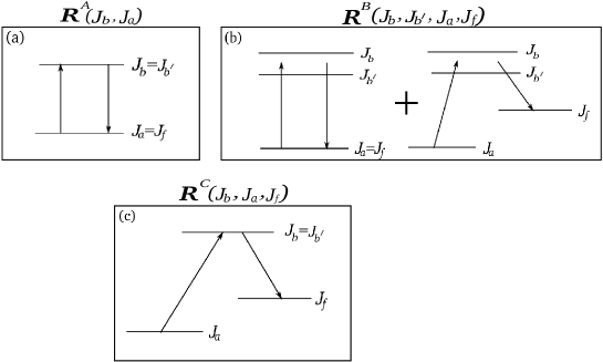
Figure 2: The schematic level diagrams representing the three components of the $J$-state redistribution matrix. Panels (a), (b), and (c) represent respectively the two-level atom resonance scattering, $J$-state interference, and Raman scattering (resonance fluorescence).

The second term represents only the $J$-state interference between different lines of the multiplet (see Figure 2b). It includes both the ‘Resonance’ and the ‘Raman’ scattering parts and is effective mainly in the wings between the lines. This term is quite insensitive to the strength of the magnetic field. This can be seen from Figures 2 and 3 of P1 where the magnetic field effects are confined mainly to the line cores. Hence in this component we can set the magnetic field equal to zero as a good approximation. This makes the evaluation of both the Resonance and the Raman scattering parts similar to that performed in P2 and P3. In the reduced basis this term is simply given by a $(6\times 6)$ matrix ${{\bm{\mathcal{R}}}^{\rm B}(x,x^{\prime})}$ which is equal to $\rm{diag}({\mathcal{R}}^{0},{\mathcal{R}}^{2},0,0,0,0)$. Here ${\mathcal{R}}^{K}$ are the redistribution functions which include the effects of collisions and the $J$-state interference between different line components in a multiplet defined in Equation (108). Only $J_{b}\neq J_{b}^{\prime}$ terms are retained in the summations appearing in this equation. The $J_{b}=J_{b^{\prime}}$ contributions are contained in the first term. However in some of the well known examples in the second solar spectrum like the Mg ii h and k, Ca ii H and K and the Cr i triplet, the initial and the final states are the same. Also for the case of the hypothetical doublet considered in this paper, arising due to an $L=0\to 1\to 0$ scattering transition with spin $S=1/2$, the initial and the final states are the same. Hence the Raman scattering part does not play a role.

The third term represents the case of only Raman scattering without the $J$-state interference, where the initial and the final states are different (see Figure 2c). A derivation of the weak field analogue of this component (in a way similar to that of Bommier [15]) is yet to be performed. Again for some of the well known examples mentioned above, this component does not contribute. Thus the final expression for the redistribution matrix that is used in Equation (99) is

$${\bm{\mathcal{R}}}(x,x^{\prime},\bm{B})\approx{\bm{\mathcal{R}}}^{\rm A}(x,x^{\prime},\bm{B})+{\bm{\mathcal{R}}}^{\rm B}(x,x^{\prime}).$$ (114)

5 Results and discussion

In this section, we study the effects of collisional redistribution matrix on the emergent Stokes profiles for the case of single scattering and also multiple scattering in an isothermal atmospheric slab. All the profiles presented in this paper are computed for a hypothetical doublet line system with the line center wavelengths at 5000 Å and 5001 Å arising due to an $L=0\to 1\to 0$ scattering transition with spin $S=1/2$. The $J$ quantum numbers of the lower and upper states are $J_{a}=J_{f}=1/2$ and $J_{b}=1/2,3/2$. In Section 5.1 we present the scattered Stokes profiles resulting in a single $90^{\circ}$ scattering case. In Section 5.2 we present the multiply scattered Stokes profiles emerging from an isothermal constant property atmospheric slab with and without the presence of a magnetic field.

5.1 The single $90^{\circ}$ scattering case

To explore the general behavior of the redistribution matrix in the presence of collisions we illustrate the Stokes profiles that result from single $90^{\circ}$ scattering event. We examine the influence of the elastic collisions on the Stokes profiles in the presence of a magnetic field. The magnetic field orientation is given by $\vartheta_{B}=90^{\circ}$ and $\varphi_{B}=45^{\circ}$ where the colatitude $\vartheta_{B}$ and azimuth $\varphi_{B}$ characterize the magnetic field orientation with respect to the polar $z$-axis (see Figure 1 of P1). We consider an unpolarized (${\bm{I}_{in}}=[1,0,0,0]^{\rm T}$) and spectrally flat (frequency independent) radiation field that is incident in the vertical direction (parallel to the polar $z$-axis). The singly scattered Stokes vectors are then exclusively determined by the first column of the angle-dependent redistribution matrix by integrating over the incident wavelengths. However in the multiple scattered solutions discussed in Section 5.2, we restrict our attention only to the angle-averaged redistribution matrix. The magnetic field strength is parametrized by the splitting parameter $v_{\rm H}$ given by

$$v_{\rm H}=\frac{\lambda_{0}^{2}e_{0}B}{4\pi mc^{2}}\times\frac{1}{\Delta\lambda_{\rm D}},$$ (115)

Figure 3: Effect of collisions: The profiles of the intensity $I$ and the fractional polarizations $-Q/I,-U/I$ and $V/I$ are plotted for a hypothetical doublet at 5000  Å and 5001  Å with field strength parameter $v_{\rm H}=0.004$. The coherence fractions used are $\gamma_{coh}=0.9$ (thick solid line), $\gamma_{coh}=0.5$ (dotted line), and $\gamma_{coh}=0.1$ (dashed line). The fine structure splitting is 1 Å. Single $90^{\circ}$ scattering is assumed at the extreme solar limb ($\mu=0$). The model parameters are $a_{R}=0.001$, $\vartheta_{B}=90^{\circ}$ and $\varphi_{B}=45^{\circ}$. The Doppler width $\Delta\lambda_{\rm D}=0.025$ Å.

where $B$ is the magnetic field strength, $e_{0}$ is the charge of the electron and $m$ its mass. $\Delta\lambda_{\rm D}$ is the Doppler width and is assumed to be 0.025 Å for both the lines. The radiative width of the upper state is parametrized as $a_{Rb}=\Gamma_{Rb}/(4\pi\Delta\nu_{\rm D})$. It is assumed to be the same for both the lines and is chosen to be 0.001. The radiative width $a_{Rb}$ is related to the total damping parameter through

$$a_{b}=a_{Rb}\Big{[}1+\Big{(}\frac{\Gamma_{Ib}+\Gamma_{E}}{\Gamma_{Rb}}\Big{)}\Big{]}.$$ (116)

We assume the inelastic collision rate $\Gamma_{Ib}$ to be zero.

The depolarizing collisional rates $D^{(2)}=0.5\Gamma_{E}$, and $D^{(0)}=0$. For simplicity we set $D^{(1)}=D^{(2)}$. However in general they can differ (for example, $D^{(1)}=0.43\Gamma_{E}$ and $D^{(2)}=0.38\Gamma_{E}$ according to Berman & Lamb [32]). We have verified that the Stokes $V/I$ is insensitive to the values of $D^{(1)}$.

The collisional effects are built into the ${\bf R}$ matrix derived in Section 3 through the branching ratios defined in Equations (67) and (68). The elastic collision rate is parametrized through the coherence fraction $\gamma_{coh}$ as $\gamma_{coh}=1/[1+(\Gamma_{E}/\overline{\Gamma}_{R}^{b{b^{\prime}}})].$ In the present paper we take $\Gamma_{R}$ to be the same for both the upper fine structure states and $\gamma_{coh}$ to be the same for all $J_{b}J_{b^{\prime}}$ combinations. When $\gamma_{coh}=1$ the redistribution is entirely radiative (only ${\bf R}^{\rm II}$), whereas $\gamma_{coh}=0$ represents purely collisional redistribution (only ${\bf R}^{\rm III}$). We consider a range of values $\gamma_{coh}\in[1,0]$ to represent an arbitrary mix of ${\bf R}^{\rm II}$ and ${\bf R}^{\rm III}$ type redistribution.

Figure 3 shows the Stokes $(I,Q/I,U/I,V/I)$ spectra for a doublet. The polarization of the line at 5001 Å is zero because its polarizability factor $W_{2}=0$. The collisions affect the wavelength domain outside the line core region of this line. But for the line at 5000 Å, the collisional effects are seen both in the line wings and the line core. In the line core the collisional effects compete with the Hanle effect and in the wings it is an interplay between the $J$-state interference effect and the collisional redistribution effect.

The value $\gamma_{coh}=0.9$ corresponds to a mix with $90\%$ of ${\bf R}^{\rm II}$ and 10% of ${\bf R}^{\rm III}$ (see the thick solid line in Figure 3). The profiles look similar to those for pure ${\bf R}^{\rm II}$ (see dotted line in Figure 3 of P1). However, in $Q/I$ there is a small depolarization, mainly in the wings, due to the presence of collisions. The core of the line at 5000 Å seems to be less affected than its wings. The $Q/I$ at the 5001 Å line remains zero. In the presence of elastic collisions, a small $U/I$ signal is generated in the wings of the 5000 Å line. This non-zero $U/I$ wing polarization and the depolarization in the wings of $Q/I$ are induced by the elastic collisions in combination with the magnetic field and can together be referred to as the ‘wing Hanle effect’. This effect arises because the elastic collisions can transfer the Hanle rotation (of the plane of polarization) from the line core to the line wings before spontaneous de-excitation intervenes. In other words, in the presence of a small but significant elastic collision rate the Hanle effect does not vanish in the line wings. If the elastic collision rate is large then the collisions completely depolarize the scattered radiation throughout the line profile. This effect has been discussed in detail in HZ2 for the case of a $J=0\to 1\to 0$ single scattering transition. However, these effects do not survive when the radiative transfer effects with angle-averaged PRD are explicitly taken into account. The collisional redistribution process is more effective in the case of angle-dependent PRD than in the case of angle-averaged PRD. Using the domain-based PRD theory of Bommier [15] this effect was noticed even in the radiative transfer computations of Nagendra et al. [33] (see also Nagendra et al. [34]). It remains as effective in a pair of interfering doublet lines as in the case of a single line. However, in Sampoorna et al. [35] it was shown that the wing Hanle effect alone is insufficient to explain the observed wing signatures in the $Q/I$ and $U/I$ profiles of the Ca i 4227 Å line.

As $\gamma_{coh}$ decreases to 0.5, which represents an equal mix of ${\bf R}^{\rm II}$ and ${\bf R}^{\rm III}$, the values of $Q/I$ in the wings of both the lines are significantly reduced (see dotted line in Figure 3). The collisional effects are now seen even in the core of the 5000 Å line. This results in a decrease of the $Q/I$ and $U/I$ signals at the center of this line. The $J$-state interference signatures in $Q/I$ are also modified. When $\gamma_{coh}$ is further reduced to 0.1, the effects of ${\bf R}^{\rm III}$ start to dominate over those of ${\bf R}^{\rm II}$ and also over the $J$-state interference effects (see dashed line in Figure 3). As a result the signatures of the $J$-state interference begin to fade away. The $Q/I$ and $U/I$ start to approach zero throughout the line profiles. As $\gamma_{coh}$ is further decreased to 0.0001 (not shown in the figure), the collisional effects (through ${\bf R}^{\rm III}$) completely dominate the scattering process. This situation corresponds to a regime of extremely large line broadening. As a result the amplitude of $I$ becomes much smaller compared to the other cases. Also, the $Q/I,U/I$, and $V/I$ approach zero level throughout the line profiles.

5.2 Polarized line profiles formed due to multiple scattering in an atmospheric slab

Figure 4: Emergent Stokes profiles at $\mu=0.047$ computed for a slab of optical thickness $T=2\times 10^{4}$ in the absence of a background continuum. The other model parameters are $(a,\epsilon)=(10^{-3},10^{-4})$. The magnetic field strength is set to zero. The coherence fraction is $\gamma_{coh}=0.1$ (solid line), $\gamma_{coh}=0.5$ (dotted line), $\gamma_{coh}=0.9$ (dashed line), and $\gamma_{coh}=1$ (dot-dashed line).

In this section we present the emergent Stokes profiles computed by solving the polarized radiative transfer equation for a two-term atom including the effects of $J$-state interference and elastic collisions. For this we consider an isothermal constant property atmospheric slab with a given optical thickness $T$. The slabs are assumed to be self-emitting. The atmospheric model parameters used for the computations are represented by $(T,a,\epsilon)$, where $a$ is the damping parameter and $\epsilon$ is the thermalization parameter defined in Equation (100) and the paragraph that follows.

The Planck function $B$ is taken as unity. The Doppler width for both the lines are assumed to be the same and equal to 0.025 Å. For more details on the structure of the atmospheric slabs and the model parametrization we refer to P2.

5.2.1 The non-magnetic case

Figure 4 shows the emergent Stokes profiles which include the effects of $J$-state interference, elastic collisions and radiative transfer computed for a model atmosphere with parameters $T=2\times 10^{4},a=10^{-3}$ and $\epsilon=10^{-4}$ in the absence of a background continuum. In these profiles the magnetic field is set to zero. Different line types represent different values of the coherence fraction $\gamma_{coh}$. A range of values of $\gamma_{coh}\in[1,0]$ is considered. As seen from the Figure 4, a decrease in $\gamma_{coh}$ results in a gradual decrease in $Q/I$ in the line core as well as in the PRD peaks of the 5000 Å line. The intensity profiles are also quite sensitive to the effect of elastic collisions. As $\gamma_{coh}$ goes from 1 (pure $\bf R^{\rm II}$ case) to 0.1 ($\bf R^{\rm III}$ dominated case), the self-reversed emission lines change over to nearly true absorption lines (thick solid lines). In $Q/I$ the effects of collisions are confined only to the line core and the near wing PRD peaks. Specifically, it is shown by Nagendra [36] that the elastic collisions $D^{(2)}$ depolarizes the line core, and $\Gamma_{E}$ significantly depolarizes the line wing polarization (See Faurobert-Scholl [37]). The same conclusions are valid in the two-term atom model also. The interference region between the two lines seems to be less sensitive to the effect of elastic collisions.

Figure 5: Same as Figure 4 but computed for an optical thickness $T=2\times 10^{8}$.

However for larger optical depths, significant dependence on $\gamma_{coh}$ is exhibited in the wavelength region between the two lines. This can be seen in Figure 5 which shows the effect of elastic collisions in an optically thick atmospheric slab in the absence of a magnetic field. The model parameters are the same as in Figure 4 but with $T=2\times 10^{8}$. As $\gamma_{coh}$ decreases, the collisions take over the line formation process. When $\gamma_{coh}=0.1$ (thick solid line), deep absorption lines are formed in $I$ with broad wings. The $Q/I$ at the center of the 5000 Å line becomes very small like in Figure 4. The zero crossing point at 5000.3 Å remains the same for all the values of $\gamma_{coh}$. In general a depolarization in $Q/I$ is seen throughout the line profile because the radiative transfer effect is significant at all the frequencies. As expected, the $Q/I$ reaches zero very far in the wings of both the lines after exhibiting a wing maximum nearly 10 Å away from their line centers. The difference in behavior in the line core as well as in the line wings of the $Q/I$ profiles formed under $\bf R^{\rm II}$ dominated (dot-dashed line) and $\bf R^{\rm III}$ dominated (thick solid line) conditions are better seen for the $T=2\times 10^{8}$ case when compared to the $T=2\times 10^{4}$ case.

5.2.2 The magnetic case

Figure 6 shows a comparison between the emergent Stokes profiles computed with (dashed line) and without (solid line) the presence of a weak magnetic field including the effects of elastic collisions. The magnetic profiles are computed for a field strength of $v_{\rm H}=0.004$ with $\gamma_{coh}=0.9$. The model parameters are $T=2\times 10^{4}$, $\epsilon=10^{-4}$, $a=10^{-3}$ in the absence of a background continuum. An external weak magnetic field (through the Hanle effect) affects the multiply scattered Stokes profiles in a way similar to the singly scattered Stokes profiles. The Hanle effect causes a depolarization in $Q/I$ at the center of the 5000 Å line and also generates a $U/I$ signal at this line. We recall that these effects are not seen at the 5001 Å line since its polarizability factor $W_{2}=0$. Like in the case of single scattered profiles, the magnetic field effects are confined only to the line core and the $J$-state interference signatures remain unaffected by the magnetic field. Also as discussed earlier, the wing Hanle effect in $Q/I$ and $U/I$ which were seen in the case of single scattered profiles in Figure 3 now disappear due to the radiative transfer effects.

Figure 6: Emergent Stokes profiles at $\mu=0.047$ computed for a magnetic field strength of $v_{\rm H}=0$ (solid line) and $v_{\rm H}=0.004$ (dashed line) with a coherence fraction $\gamma_{coh}=0.9$ in the absence of a background continuum. The model parameters are $(T,a,\epsilon)=(2\times 10^{4},10^{-3},10^{-4})$.

6 Conclusions

In the present paper we have extended the theoretical framework for the $J$-state interference for type-II redistribution developed in P1, to include the effects of collisions (type-III redistribution). The collisional PRD matrix is derived in the laboratory frame for a two-term atom with an unpolarized lower term and in the presence of magnetic fields of arbitrary strengths. However, the treatment is restricted to the linear Zeeman regime for which the Zeeman splitting is much smaller than the fine-structure splitting. The inelastic collisions coupling the upper term and the lower term and also the inelastic collisions coupling the fine structure states of the upper term are taken into account. However, the latter has been treated approximately. The approximation involves considering only the depolarizing effects of the inelastic collisions but neglecting the polarization transfer rates between the fine structure states. The depolarization caused by the inelastic collisions has the same type of consequences as the depolarization by elastic collisions. Therefore we can merge both these effects into a common damping rate for the state $J_{b}$ and appropriately redefine the branching ratios and the thermalization parameter for a two-term atom. A proper treatment of the inelastic collisions which cause polarization transfer requires formulating and solving the polarized statistical equilibrium equations. This is outside the scope of the present paper. The approximate treatment presented in this paper leads to slightly larger values of polarization in the line core as the inelastic collisions are not handled exactly. A treatment involving the statistical equilibrium equation would yield correct values of linear polarization. However in the line wings the formulation presented here becomes accurate enough and would give the same result as a full treatment in terms of statistical equilibrium equation, including PRD mechanism.

The collisional frequency shift is inherently built into the redistribution matrix through the type-III redistribution function and the branching ratios. We discuss in detail the procedure of assigning the correct multipolar index $K$ to the collisional branching ratio and depolarizing elastic collision rate $D^{(K)}$. This procedure requires a detailed understanding of the role played by the multipolar index $K$ for both the atom and the radiation field. We show how it becomes necessary to introduce a quantum generalized profile function for the case of a two-term atom in order to assign appropriate index $K$ to the branching ratios and to $D^{(K)}$. In general $D^{(K)}$ is defined for each of the fine structure components (by making it depend on the quantum number $J_{b}$). However in the present paper we assume it to be independent of the $J$-quantum number.

Examples of the Stokes profiles resulting from single $90$° scattering are illustrated for different values of the coherence fraction $\gamma_{coh}$. The profiles look similar to the ones presented in P1, which were computed using collisionless redistribution (the case of pure ${\bf R}^{\rm II}$), except for the depolarization in the wings of the $Q/I$ profiles, and non-zero polarization in the wings of the $U/I$ profiles. This interesting feature, which we refer to as the wing Hanle effect, is discussed.

The effects of collisions are discussed by incorporating the newly derived collisional redistribution matrix in the polarized radiative transfer equation, in the simpler case of isothermal slab models. The technique of incorporating the Hanle redistribution matrix with the $J$-state interference and collisions, into the polarized radiative transfer equation for a two-term atom is presented. It is shown that the effects of elastic collisions in a two-term atom are similar to those of the two-level atom case. The redistribution matrices derived here have been used in the interpretation of the quantum interference signatures seen in the limb observations of the Cr i triplet in Smitha et al. [10]. For simplicity the inelastic collisions between the fine structure states were neglected in that realistic modeling effort.

With the present work we have further extended the theoretical tools that are needed for modelling the various spectral structures arising due to the transitions between fine structure states of an atom that have been observed in the Second Solar Spectrum so that they can be used to diagnose magnetic fields in regimes not accessible to the Zeeman effect.

Appendix A Magnetic redistribution functions for type-III redistribution

In this appendix we present the expressions for the magnetic redistribution functions of the type HH, HF, FH and FF appearing in Equations (25) and (26). They are defined as follows

$$R^{\rm III,\,HH}_{b_{m}a_{m},{b^{\prime}}_{m}f_{m}}(x_{b^{\prime}f},\,x^{\prime}_{ba},\,\Theta) = {\frac{1}{\pi^{2}\sin\Theta}}\int_{-\infty}^{+\infty}du\,e^{-u^{2}}\left[{\frac{a_{b}}{a_{b}^{2}+(v^{\prime}_{b_{m}a_{m}}-u)^{2}}}\right]$$ (117)

$$\times H\left({\frac{a_{b^{\prime}}}{\sin\Theta}},\,{\frac{v_{{b^{\prime}}_{m}f_{m}}}{\sin\Theta}}-u\cot\Theta\right),$$

$$R^{\rm III,\,HF}_{b_{m}a_{m},{b^{\prime}}_{m}f_{m}}(x_{b^{\prime}f},\,x^{\prime}_{ba},\,\Theta) = {\frac{1}{\pi^{2}\sin\Theta}}\int_{-\infty}^{+\infty}\,du\,e^{-u^{2}}\,\left[{\frac{a_{b}}{a_{b}^{2}+(v^{\prime}_{b_{m}a_{m}}-u)^{2}}}\right]\,$$ (118)

$$\times 2F\left({\frac{a_{b^{\prime}}}{\sin\Theta}},\,{\frac{v_{{b^{\prime}}_{m}f_{m}}}{\sin\Theta}}-u\cot\Theta\right),$$

$$R^{\rm III,\,FH}_{b_{m}a_{m},{b^{\prime}}_{m}f_{m}}(x_{b^{\prime}f},\,x^{\prime}_{ba},\,\Theta) = {\frac{1}{\pi^{2}\sin\Theta}}\int_{-\infty}^{+\infty}\,du\,e^{-u^{2}}\,\left[{\frac{(v^{\prime}_{b_{m}a_{m}}-u)}{a_{b}^{2}+(v^{\prime}_{b_{m}a_{m}}-u)^{2}}}\right]\,$$ (119)

$$\times H\left({\frac{a_{b^{\prime}}}{\sin\Theta}},\,{\frac{v_{{b^{\prime}}_{m}f_{m}}}{\sin\Theta}}-u\cot\Theta\right),$$

and

$$R^{\rm III,\,FF}_{b_{m}a_{m},{b^{\prime}}_{m}f_{m}}(x_{b^{\prime}f},\,x^{\prime}_{ba},\,\Theta) = {\frac{1}{\pi^{2}\sin\Theta}}\int_{-\infty}^{+\infty}\,du\,e^{-u^{2}}\,\left[{\frac{(v^{\prime}_{b_{m}a_{m}}-u)}{a_{b}^{2}+(v^{\prime}_{b_{m}a_{m}}-u)^{2}}}\right]\,$$ (120)

$$\times 2F\left({\frac{a_{b^{\prime}}}{\sin\Theta}},\,{\frac{v_{{b^{\prime}}_{m}f_{m}}}{\sin\Theta}}-u\cot\Theta\right).$$

In the above equations $H(a,x)$ and $F(a,x)$ are the Voigt and Faraday-Voigt functions (see Equation (18) of P1 for their definition). $\Theta$ is the scattering angle (the angle between the incident and scattered rays; see Figure 1 of P1). The dimensionless quantities appearing in Equations (117) to (120) are given by

$$x_{ba}={\nu_{0ba}-\nu\over\Delta\nu_{\rm D}};\quad a_{b}={\frac{\gamma_{b}+\gamma_{c}}{4\pi\Delta\nu_{{\rm D}}}};\quad v_{b_{m}a_{m}}=x_{ba}+(g_{b}\mu_{b}-g_{a}\mu_{a})\frac{\nu_{L}}{\Delta\nu_{{\rm D}}},$$ (121)

where $\nu_{0ba}$ is the line center frequency corresponding to a $J_{a}\to J_{b}$ transition in the absence of magnetic fields, $a_{b}$ is the damping parameter of the excited state $b$, and ${\Delta\nu_{{\rm D}}}$ is the Doppler width. In the limit of a two-level atom (obtained by setting $J_{b}=J_{b}^{\prime}$ and $J_{a}=J_{f}$) and in the absence of a magnetic field the $R^{\rm III,\,HH}$ and $R^{\rm II,\,H}$ (defined in P1) reduce to the Hummer’s $R^{\rm III}$ and $R^{\rm II}$ functions respectively (see also HZ1).

The angle-averaged analogues of Equations (117)-(120) are obtained through

$$R^{\rm III,\,XY}_{b_{m}a_{m},{b^{\prime}}_{m}f_{m}}(x_{b^{\prime}f},\,x^{\prime}_{ba})=\frac{1}{2}\int_{0}^{\pi}R^{\rm III,\,XY}_{b_{m}a_{m},{b^{\prime}}_{m}f_{m}}(x_{b^{\prime}f},\,x^{\prime}_{ba},\,\Theta)\ \sin\Theta\ d\Theta,$$ (122)

(see Equations (103) and (104) of Bommier [15] and Equations (30) and (31) of Sampoorna et al. [38]), where X and Y stand for H and/or F. A similar expression can be used for computing angle-averaged analogues of the type-II functions.

References

- Stenflo & Keller [1996] Stenflo, J. O., & Keller, C. U. 1996, Nature, 382, 588
- Stenflo & Keller [1997] Stenflo, J. O., & Keller, C. U. 1997, A&A, 321, 927
- Stenflo et al. [1997] Stenflo J. O., Bianda, M., Keller C. U., & Solanki S. K. 1997, A&A, 322, 985
- Stenflo [1994] Stenflo, J. O. 1994, Solar Magnetic Fields: Polarized Radiation Diagnostics (Dordrecht: Kluwer) (S94)
- Stenflo [1998] Stenflo, J. O. 1998, A&A, 338, 301 (S98)
- Bommier & Stenflo [1999] Bommier, V., & Stenflo, J. O. 1999, A&A, 350, 327 (BS99)
- Sampoorna et al. [2007a] Sampoorna, M., Nagendra, K. N., & Stenflo, J. O. 2007a, ApJ, 663, 625 (HZ1)
- Sampoorna [2011] Sampoorna, M. 2011, ApJ, 731, 114
- Smitha et al. [2011a] Smitha, H. N., Sampoorna, M., Nagendra, K. N., & Stenflo, J. O. 2011a, ApJ, 733, 4 (P1)
- Smitha et al. [2012] Smitha, H. N., Nagendra, K. N., Stenflo, J. O. et al. 2012, A&A, 541, 24 (P3)
- Omont et al. [1972] Omont, A., Smith, E. W., & Cooper, J. 1972, ApJ, 175, 185
- Omont et al. [1973] Omont, A., Smith, E. W., & Cooper, J. 1973, ApJ, 182, 283
- Domke & Hubeny [1988] Domke, H., & Hubeny, I. 1988, ApJ, 334, 527
- Bommier [1997a] Bommier, V. 1997a, A&A, 328, 706
- Bommier [1997b] Bommier, V. 1997b, A&A, 328, 726
- Bommier [2003] Bommier, V. 2003, in ASP Conf. Ser. 307, Solar Polarization 3, ed. J. Trujillo Bueno & J. Sanchez Almedia, (San Francisco: ASP), 213
- Landi Degl’Innocenti et al. [1997] Landi Degl’Innocenti, E., Landi Degl’Innocenti, M., & Landolfi, M. 1997, in Proc. Forum THÉMIS, Science with THÉMIS, ed. N. Mein & S. Sahal-Bréchot (Paris: Obs. Paris-Meudon), 59
- Sampoorna et al. [2007b] Sampoorna, M., Nagendra, K. N., & Stenflo, J. O. 2007b, ApJ, 670, 1485 (HZ2)
- Kerkeni & Bommier [2002] Kerkeni, B., & Bommier, V. 2002, A&A, 394, 707
- Kerkeni [2002] Kerkeni, B. 2002, A&A, 390, 783
- Hummer [1962] Hummer, D. G. 1962, MNRAS, 125, 1
- Smitha et al. [2011b] Smitha, H. N., Nagendra, K. N., Sampoorna, M., & Stenflo, J. O. 2011b, A&A, 535, 35 (P2)
- Landi Degl’Innocenti & Landolfi [2004] Landi Degl’Innocenti, E., & Landolfi, M. 2004, Polarization in Spectral Lines (Dordrecht: Kluwer) (LL04)
- Fano [1957] Fano, U. 1957, Rev. Mod. Phys, 29, 74
- Sahal-Bréchot et al. [1977] Sahal-Bréchot, S., Bommier, V., & Leroy, J, L. 1977, A&A, 59, 223
- Trujillo Bueno [2001] Trujillo Bueno, J. 2001, in ASP Conf. Ser. 236, Advanced Solar Polarimetry: Theory, Observation and Instrumentation, ed. M. Sigwarth (San Francisco: ASP), 161
- Landi Degl’Innocenti et al. [1991] Landi Degl’Innocenti, E., Bommier, V., & Sahal-Bréchot, S. 1991 A&A, 244, 401
- Heinzel & Hubeny [1982] Heinzel, P., & Hubeny, I. 1982, JQSRT, 27, 1
- Frisch [2007] Frisch, H. 2007, A&A, 476, 665
- Landi Degl’Innocenti [1984] Landi Degl’Innocenti, E. 1984, Sol. Phys, 91, 1
- Anusha et al. [2011] Anusha, L. S., Nagendra, K .N., Bianda, M. et al. 2011, ApJ, 737, 95
- Berman & Lamb [1969] Berman, P. R., & Lamb, Willis E. Jr 1969, Phys. Rev, 187, 221
- Nagendra et al. [2002] Nagendra, K. N., Frisch, H., & Faurobert, M. 2002, A&A, 395, 305
- Nagendra et al. [2003] Nagendra, K. N., Frisch, H., & Fluri, D. M. 2003, in ASP Conf. Ser. 307, Solar Polarization 3, ed. J. Trujillo Bueno & J. Sanchez Almeida (San Francisco: ASP), 227
- Sampoorna et al. [2009] Sampoorna, M., Stenflo, J. O., Nagendra K. N. et al. 2009, ApJ, 699, 1650
- Nagendra [1994] Nagendra, K. N. 1994, ApJ, 432, 274
- Faurobert-Scholl [1992] Faurobert-Scholl, M. 1992, A&A, 258, 521
- Sampoorna et al. [2008] Sampoorna, M., Nagendra, K. N., & Stenflo, J. O. 2008, ApJ, 679, 889