Single top quark polarization at $O(\alpha_{s})$ in $t\bar{t}$ production MZ-TH/12-41 August 2012
at a polarized linear $e^{+}e^{-}$ collider

Abstract

We present a detailed investigation of the NLO polarization of the top quark in $t\bar{t}$ production at a polarized linear $e^{+}e^{-}$ collider with longitudinally polarized beams. By appropiately tuning the polarization of the beams one can achieve close to maximal values for the top quark polarization over most of the forward hemisphere for a large range of energies. This is quite welcome since the rate is largest in the forward hemisphere. One can also tune the beam polarization to obtain close to zero polarization over most of the forward hemisphere.

1 Introductory remarks

The top quark is so heavy that it keeps its polarization at production when it decays since $\tau_{\rm hadronization}\gg\tau_{\rm decay}$. One can test the Standard Model (SM) and/or non-SM couplings through polarization measurements involving top quark decays (mostly $t\to b+W^{+}$). New observables involving top quark polarization can be defined such as $\langle\vec{P}_{t}\cdot\vec{p}\rangle$ (see e.g. Refs. [1, 2, 3, 4, 5, 6]). It is clear that the analyzing power of such observables is largest for large values of the polarization of the top quark. This calls for large top quark polarization values. One also wants a control sample with small or zero top quark polarization. Near maximal and minimal values of top quark polarization at a linear $e^{+}e^{-}$ collider can be achieved in $t\bar{t}$ production by appropiately tuning the longitudinal polarization of the beam polarization [8]. At the same time one wants to keep the top quark pair production cross section large. It is a fortunate circumstance that all these goals can be realized at the same time. A polarized linear $e^{+}e^{-}$ collider may thus be viewed as a rich source of close to zero and close to $100\%$ polarized top quarks.

Let us remind the reader that the top quark is polarized even for zero beam polarization through vector–axial vector interference effects $\sim v_{e}a_{e},\,v_{e}a_{f},\,v_{f}a_{e},\,v_{f}a_{f}$, where

$$v_{e},a_{e}\quad :$$ electron current coupling

$$v_{f},a_{f}\quad :$$ top quark current coupling (1)

In Fig. 1 we present a NLO plot of the $\cos\theta$ dependence of the zero beam polarization top quark polarization for different characteristic energies at $\sqrt{s}=360$ GeV (close to threshold), $\sqrt{s}=500$ GeV (ILC phase 1), $\sqrt{s}=1000$ GeV (ILC phase 2) and $\sqrt{s}=3000$ GeV (CLIC).

Figure 1: Magnitude of NLO top quark polarization for zero beam polarization

2 Top quark polarization at threshold and in the high energy limit

The polarization of the top quark depends on the c.m. energy $\sqrt{s}$, the scattering angle $\cos\theta$, the electroweak coupling coefficients $g_{ij}$ and the effective beam polarization $P_{\rm eff}$, i.e. one has

$$\vec{P}=\vec{P}\,(\sqrt{s},\cos\theta,g_{ij},P_{\rm eff})\,,$$ (2)

where the effective beam polarization appearing in Eq. (2) is given by [9]

$$P_{\rm eff}=\frac{h_{-}-h_{+}}{1-h_{-}h_{+}}\,.$$ (3)

and where $h_{-}$ and $h_{+}$ are the longitudinal polarization of the electron and positron beams $(-1<h_{\pm}<+1)$, respectively. Instead of the nonchiral electroweak couplings $g_{ij}$ one can alternatively use the chiral electroweak couplings $f_{mm^{\prime}}$ ($m,m^{\prime}=L,R$) introduced in Refs. [11, 12]. The relations between the two sets of electroweak coupling coefficients can be found in Ref. [8]. In this report we shall make use of both sets of coupling parameters.

For general energies the functional dependence in Eq. (2) is not simple. Even if the electroweak couplings $g_{ij}$ are fixed, one remains with a three-dimensional parameter space $(\sqrt{s},\cos\theta,P_{\rm eff})$. Our strategy is to discuss various limiting cases for the Born term polarization and then to investigate how the limiting values extrapolate away from these limits. In particular, we exploit the fact that, in the Born term case, angular momentum conservation (or $m$-quantum number conservation) implies $100\%$ top quark polarization at the forward and backward points for the $(e^{-}_{L}e^{+}_{R})$ and $(e^{-}_{R}e^{+}_{L})$ beam configurations.

In this section we discuss the behaviour of $\vec{P}$ at nominal threshold $\sqrt{s}=2m_{t}$ ($v=0$) and in the high energy limit $\sqrt{s}\to\infty$ ($v\to 1$). At threshold and at the Born term level one has

$$\vec{P}_{\rm thresh}=\frac{P_{\rm eff}-A_{LR}}{1-P_{\rm eff}A_{LR}}\,\,\,\hat{n}_{e^{-}}\,,$$ (4)

where $A_{LR}$ is the left–right beam polarization asymmetry $(\sigma_{LR}-\sigma_{RL})/(\sigma_{LR}+\sigma_{RL})$ and $\hat{n}_{e^{-}}$ is a unit vector pointing into the direction of the electron momentum. We use a notation where $\sigma(LR/RL)=\sigma(h_{-}=\mp 1;h_{+}=\pm 1)$. In terms of the electroweak coupling parameters $g_{ij}$, the nominal polarization asymmetry at threshold $\sqrt{s}=2m_{t}$ is given by $A_{LR}=-(g_{41}+g_{42})/(g_{11}+g_{12})=0.409$. Eq. (4) shows that, at threshold and at the Born term level, the polarization $\vec{P}$ is parallel to the beam axis irrespective of the scattering angle and has maximal values $|\vec{P}|=1$ for both $P_{\rm eff}=\pm 1$ as dictated by angular momentum conservation. Zero polarization is achieved for $P_{\rm eff}=A_{LR}=0.409$.

In the high energy limit the polarization of the top quark is purely longitudinal, i.e. the polarization points into the direction of the top quark. At the Born term level one finds $\vec{P}(\cos\theta)=P^{(\ell)}(\cos\theta)\cdot\hat{p_{t}}$ with

$$P^{(\ell)}(\cos\theta)=\frac{(g_{14}+g_{41}+P_{\rm eff}(g_{11}+g_{44}))(1+\cos\theta)^{2}+(g_{14}-g_{41}-P_{\rm eff}(g_{11}-g_{44})(1-\cos\theta)^{2}}{(g_{11}+g_{44}+P_{\rm eff}(g_{14}+g_{41}))(1+\cos\theta)^{2}+(g_{11}-g_{44}-P_{\rm eff}(g_{14}-g_{41}))(1-\cos\theta)^{2}}\,.$$ (5)

In the same limit, the electroweak coupling coefficients appearing in Eq. (5) take the numerical values $g_{11}=0.601$, $g_{14}=-0.131$, $g_{41}=-0.201$ and $g_{44}=0.483$. For $\cos\theta=\pm 1$ and $P_{\rm eff}=\pm 1$ the top quark is $100\%$ polarized as again dictated by angular momentum conservation. The lesson from the threshold and high energy limits is that large values of the polarization of the top quark close to $|\vec{P}|=1$ are engendered for large values of the effective beam polarization parameter close to $P_{\rm eff}=\pm 1$.

Take, for example, the forward–backward asymmetry which is zero at threshold, and large and positive in the high energy limit. In fact, from the numerator of the high energy formula Eq. (5) one calculates

$$A_{FB}=\frac{3}{4}\,\,\frac{g_{44}+P_{\rm eff}g_{14}}{g_{11}+P_{\rm eff}g_{41}}\,=\,0.61\,\frac{1-0.27P_{\rm eff}}{1-0.33P_{\rm eff}}\,.$$ (6)

The forward-backward asymmetry is large and only mildly dependent on $P_{\rm eff}$. More detailed calculations show that the strong forward dominance of the rate sets in rather fast above threshold [8]. This is quite welcome since the forward region is also favoured from the polarization point of view.

As another example take the vanishing of the polarization which, at threshold, occurs at $P_{\rm eff}=0.409$. In the high energy limit, and in the forward region where the numerator part of Eq. (5) proportional to $(1+\cos\theta)^{2}$ dominates, one finds a polarization zero at $P_{\rm eff}=(g_{14}+g_{41})/(g_{11}+g_{44})=0.306$. The two values of $P_{\rm eff}$ do not differ much from another.

3 Overall rate and left-right (LR) and right-left (RL) rates

The overall rate $\sigma$ for partially longitudinal polarized beam production can be composed from the LR rate $\sigma_{LR}$ and the RL rate $\sigma_{RL}$ valid for $100\%$ longitudinally polarized beams. The notation is such that LR and RL refer to the $(e^{-}_{L}e^{+}_{R})$ and $(e^{-}_{R}e^{+}_{L})$ longitudinal polarization configurations, respectively. The relation reads [10]

$$\frac{d\sigma}{d\cos\theta} = \frac{1-h_{-}}{2}\frac{1+h_{+}}{2}\frac{d\sigma_{LR}}{d\cos\theta}+\frac{1+h_{-}}{2}\frac{1-h_{+}}{2}\frac{d\sigma_{RL}}{d\cos\theta}$$ (7)

$$= \frac{1}{4}(1-h_{-}h_{+})\Big{(}\frac{d\sigma_{LR}+d\sigma_{RL}}{d\cos\theta}-P_{\rm eff}\frac{d\sigma_{LR}-d\sigma_{RL}}{d\cos\theta}\Big{)}\,.$$

Using the left–right polarization asymmetry

$$A_{LR}=\frac{d\sigma_{LR}-d\sigma_{RL}}{d\sigma_{LR}+d\sigma_{RL}}$$ (8)

one can rewrite the rate (7) in the form

$$\frac{d\sigma}{d\cos\theta}=\frac{1}{4}(1-h_{-}h_{+})\frac{d\sigma_{LR}+d\sigma_{RL}}{d\cos\theta}\Big{(}1-P_{\rm eff}A_{LR}\Big{)}\,.$$ (9)

The differential rate $d\sigma/d\cos\theta$ carries an overall helicity alignment factor $(1-h_{-}h_{+})$ which enhances the rate for negative values of $h_{-}h_{+}$. Also, Fig. 2 shows that $A_{LR}$ varies in the range between $0.30$ and $0.60$ which leads to a further rate enhancement from the last factor in Eq. (9) for negative values of $P_{\rm eff}$.

Figure 2: NLO left–right polarization asymmetry $A_{LR}$ for $\sqrt{s}=360$, $500$, $1000$, and $3000$ GeV

Let us define reduced LR and RL rate functions $D_{LR/RL}$ by writing

$$\frac{d\sigma_{LR/RL}}{d\cos\theta}=\frac{\pi\alpha^{2}v}{3s^{2}}D_{LR/RL}(\cos\theta)$$ (10)

such that, in analogy to Eq. (7),

$$D=\frac{1}{4}(1-h_{-}h_{+})\left(D_{LR}+D_{RL}-P_{\rm eff}(D_{LR}-D_{RL})\right)\,.$$ (11)

In the next step we express the reduced rate functions through a set of independent hadronic helicity structure functions. For the LR reduced rate function one has

$$2D_{LR}(\cos\theta) = \frac{3}{8}(1+\cos^{2}\theta)\left((f_{LL}^{2}+f_{LR}^{2})H_{U}^{1}+2f_{LL}f_{LR}H_{U}^{2}\right)$$ (12)

$$+\frac{3}{4}\sin^{2}\theta\left((f_{LL}^{2}+f_{LR}^{2})H_{L}^{1}+2f_{LL}f_{LR}H_{L}^{2}\right)$$

$$+\frac{3}{4}\cos\theta(f_{LL}^{2}-f_{LR}^{2})H_{F}^{4}$$

and accordingly for $D_{RL}$ with $f_{LL}\to f_{RR}$ and $f_{LR}\to f_{RL}$.

At NLO one has $H_{a}^{j}=H_{a}^{j}({\it Born\/})+H_{a}^{j}(\alpha_{s})$. The radiatively corrected structure functions $H_{a}^{j}(\alpha_{s})$ are listed in Ref. [8]. If needed they can be obtained from S.G. or B.M. in Mathematica format. For the non-vanishing unpolarized Born term contributions $H_{a}^{j}({\it Born\/})$ one obtains (see e.g. Ref. [7, 8])

$$H_{U}^{1}({\it Born\/})=2N_{c}s(1+v^{2}), H_{L}^{1}({\it Born\/})=\ H_{L}^{2}({\it Born\/})=N_{c}s(1-v^{2}),$$

$$H_{U}^{2}({\it Born\/})=2N_{c}s(1-v^{2}), H_{F}^{4}({\it Born\/})=4N_{c}sv.$$ (13)

Following Refs. [11, 12], $D_{LR}(\cos\theta)$ (and $D_{RL}(\cos\theta)$) can be cast into a very compact Born term form

$$D_{LR}(Born)=\frac{3}{8}\left(C_{LR}^{2}-2f_{LL}f_{LR}v^{2}\sin^{2}\theta\right)2N_{c}s,$$ (14)

where

$$C_{LR}(\cos\theta)=f_{LL}(1+v\cos\theta)+f_{LR}(1-v\cos\theta)\,.$$ (15)

The corresponding RL form $D_{RL}$ is obtained again by the substitution $(L\leftrightarrow R)$ in Eqs. (14) and (15).

With the help of the compact expression in Eq. (14) and the translation table $2(g_{11}-g_{41})=(f_{LL}^{2}+f_{LR}^{2})$, $2(g_{14}-g_{44})=-f_{LL}^{2}+f_{LR}^{2}$, $2(g_{11}+g_{41})=f_{RR}^{2}+f_{RL}^{2}$, $2(g_{14}+g_{44})=f_{RR}^{2}-f_{RL}^{2}$ one can easily verify the threshold value for $A_{LR}$ and the high energy limits for $A_{FB}$ discussed in Sec. 2.

4 Single top polarization in $e^{+}e^{-}\to t\bar{t}$

The polarization components $P^{(m)}$ ($m=\ell$: longitudinal; $m=tr$: transverse) of the top quark in $e^{+}e^{-}\to t\bar{t}$ are obtained from (the antitop quark spin is summed over)

$$P^{(m)}(P_{\rm eff})=\frac{N^{(m)}(P_{\rm eff})}{D(P_{\rm eff})}\,,$$ (16)

where the dependence on $P_{\rm eff}$ is given by

$$N^{(m)}(P_{\rm eff})=\frac{1}{4}(1-h_{-}h_{+})\left(N^{(m)}_{LR}+N^{(m)}_{RL}-P_{\rm eff}(N^{(m)}_{LR}-N^{(m)}_{RL})\right)\,.$$ (17)

$P^{(tr)}$ is the transverse polarization component perpendicular to the momentum of the top quark in the scattering plane. The overall helicity alignment factor $(1-h_{-}h_{+})$ drops out when one calculates the normalized polarization components according to Eq. (16). This explains why the polarization depends only on $P_{\rm eff}$ and not separately on $h_{-}$ and $h_{+}$ (see Eq. (2)).

The numerator factors $N^{(m)}_{LR}$ and $N^{(m)}_{RL}$ in Eq. (16) are given by

$$-2N^{(\ell)}_{LR}(\cos\theta) = \frac{3}{8}(1+\cos^{2}\theta)\,(f_{LL}^{2}-f_{LR}^{2})H_{U}^{4(\ell)}+\frac{3}{4}\sin^{2}\theta\,(f_{LL}^{2}-f_{LR}^{2})H_{L}^{4(\ell)}$$ (18)

$$+\frac{3}{4}\cos\theta\,\bigg{(}(f_{LL}^{2}+f_{LR}^{2})H_{F}^{1(\ell)}+2f_{LL}f_{LR}H_{F}^{2(\ell)}\bigg{)}\,,$$

$$-2N^{(tr)}(\cos\theta)\!\!\! = \!\!\!-\frac{3}{\sqrt{2}}\sin\theta\cos\theta\,\,(f_{LL}^{2}-f_{LR}^{2})\,H_{I}^{4(tr)}$$ (19)

$$-\frac{3}{\sqrt{2}}\sin\theta\left((f_{LL}^{2}+f_{LR}^{2})H_{A}^{1(tr)}+2f_{LL}f_{LR}H_{A}^{2(tr)}\right)\,,$$

and $N^{(m)}_{RL}=-N^{(m)}_{LR}(L\leftrightarrow R)$. Note the extra minus sign when relating $N^{(m)}_{LR}$ and $N^{(m)}_{RL}$.

The LO longitudinal and transverse polarization components read (see e.g. Ref. [7, 8])

$$H_{U}^{4(\ell)}({\it Born\/})=4N_{c}sv, H_{F}^{1(\ell)}({\it Born\/})=2N_{c}s(1+v^{2}),$$

$$H_{L}^{4(\ell)}({\it Born\/})=0, H_{F}^{2(\ell)}({\it Born\/})=2N_{c}s(1-v^{2}),$$ (20)

and

$$H_{I}^{4(tr)}({\it Born\/})=2N_{c}s\frac{1}{2\sqrt{2}}v\sqrt{1-v^{2}},\quad H_{A}^{1(tr)}({\it Born\/})=H_{A}^{2(tr)}({\it Born\/})=2N_{c}s\frac{1}{2\sqrt{2}}\sqrt{1-v^{2}}\,.$$ (21)

The LO numerators (18) and (19) can be seen to take a factorized form [11, 12]

$$N_{LR}^{(\ell)}(\cos\theta) = -\frac{3}{8}\bigg{(}f_{LL}(\cos\theta+v)+f_{LR}(\cos\theta-v)\bigg{)}\,C_{LR}(\cos\theta)\,\,2N_{c}s\,,$$

$$N_{LR}^{(tr)}(\cos\theta) = \frac{3}{8}\sin\theta\sqrt{1-v^{2}}\,(f_{LL}+f_{LR})\,C_{LR}(\cos\theta)\,\,2N_{c}s\,,$$ (22)

where the common factor $C_{LR}(\cos\theta)$ has been defined in Eq. (15).

One can then determine the angle $\alpha$ enclosing the direction of the top quark and its polarization vector by taking the ratio $N^{(tr)}_{LR}/N^{(\ell)}_{LR}$. One has

$$\tan\alpha_{LR}=\frac{N_{LR}^{(tr)}(\cos\theta)}{N_{LR}^{(\ell)}(\cos\theta)}=-\frac{\sin\theta\sqrt{1-v^{2}}\,(f_{LL}+f_{LR})}{f_{LL}(\cos\theta+v)+f_{LR}(\cos\theta-v)}\,.$$ (23)

For $v=1$ one finds $\alpha_{LR}=0$, i.e. the polarization vector is aligned with the momentum of the top quark, in agreement with what has been said before. In Ref. [8] we have shown that radiative corrections to the value of $\alpha_{LR}$ are small in the forward region but can become as large as $\Delta\alpha_{LR}=10^{\circ}$ in the backward region for large energies.

Eqs. (4) and (22) can be used to find a very compact LO form for $|\vec{P}_{LR}|$. One obtains [8]

$$|\vec{P}_{LR}|=\frac{\sqrt{N_{LR}^{(\ell)2}+N_{LR}^{(tr)2}}}{D_{LR}}=\frac{\sqrt{1-4a_{LR}}}{1-2a_{LR}}=1-2a_{LR}^{2}-8a_{LR}^{3}-18a_{LR}^{3}\ldots,$$ (24)

where the coefficient $a_{LR}$ depends on $\cos\theta$ through

$$a_{LR}(\cos\theta)=\frac{f_{LL}f_{LR}}{C_{LR}^{2}(\cos\theta)}v^{2}\sin^{2}\theta\,.$$ (25)

Again, the corresponding expressions for $|\vec{P}_{LR}|$ and $a_{LR}$ can be found by the substitution $(L\leftrightarrow R)$.

For the fun of it we also list a compact LO form for $|\vec{P}(P_{\rm eff}=0)|$. One has

$$|\vec{P}(P_{\rm eff}=0)|=\frac{\sqrt{(C_{LR}^{2}-C_{RL}^{2})^{2}-4v^{2}\sin^{2}\theta(C_{LR}f_{LL}-C_{RL}f_{RR})(C_{LR}f_{LR}-C_{RL}f_{RL})}}{C_{LR}^{2}+C_{RL}^{2}-2v^{2}\sin^{2}\theta(f_{LL}f_{LR}+f_{RR}f_{RL})}\,.$$ (26)

Eq. (26) would produce a LO version of Fig 1.

5 Effective beam polarization

As described in Sec. 2, large values of the effective beam polarization $P_{\rm eff}$ are needed to produce large polarization values of $\vec{P}$. It is a fortunate circumstance that nearly maximal values of $P_{\rm eff}$ can be achieved with non-maximal values of $(h_{-},h_{+})$. This is shown in Fig. 3 where we drawn contour plots $P_{\rm eff}={\it const}$ in the $(h_{-},h_{+})$ plane. The two examples shown in Fig. 3 refer to

$$(h_{-}=-0.80,\,h_{+}=+0.625)\qquad\mbox{leads to}\quad P_{\rm eff}=-0.95,$$

$$(h_{-}=+0.80,\,h_{+}=-0.625)\qquad\mbox{leads to}\quad P_{\rm eff}=+0.95.$$ (27)

These two options are at the technical limits that can be achieved [13]. In the next section we shall see that the choice $P_{\rm eff}\sim-0.95$ is to be preferred since the polarization is more stable against small variations of $P_{\rm eff}$. Furthermore, negative values of $P_{\rm eff}$ gives yet another rate enhancement as discussed after Eq. (9).

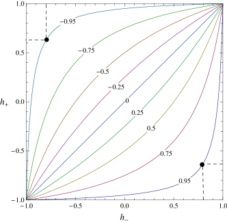
Figure 3: Contour plots of $P_{\rm eff}={\it const}$ in the $(h_{+},h_{-})$ plane

6 Stability of polarization against variations of $P_{\rm eff}$

Extrapolations of $|\vec{P}|$ away from $P_{\rm eff}=\pm 1$ are more stable for $P_{\rm eff}=-1$ than for $P_{\rm eff}=+1$. Because the derivative of the magnitude of $|\vec{P}|$ leads to rather unwieldy expressions, we demonstrate this separately for the two polarization components $P^{(\ell)}$ and $P^{(tr)}$. The polarization components are given by ($m=\ell,tr$)

$$P^{(m)}=\frac{N_{0}^{(m)}-P_{\rm eff}N_{P}^{(m)}}{D_{0}-P_{\rm eff}D_{P}}\,,$$ (28)

where $N_{0}^{(m)}=N_{LR}^{(m)}+N_{RL}^{(m)}$ and $N_{P}^{(m)}=N_{LR}^{(m)}-N_{RL}^{(m)}$ and similarly for $D_{0}$ and $D_{P}$. Upon differentiation w.r.t. $P_{\rm eff}$ one obtains

$$\frac{dP^{(m)}\,}{dP_{\rm eff}}=\frac{-N_{0}^{(m)}D_{P}+N_{P}^{(m)}D_{0}}{\left(D_{0}-P_{\rm eff}D_{P}\right)^{2}}\,.$$ (29)

For the ratios of the slopes for $P_{\rm eff}=-1$ and $P_{\rm eff}=+1$ one finds

$$\frac{dP^{(m)}\,}{dP_{\rm eff}}\Big{|}_{P_{\rm eff}=-1}\,\bigg{/}\,\frac{dP^{(m)}\,}{dP_{\rm eff}}\Big{|}_{P_{\rm eff}=+1}=\left(\frac{D_{0}-D_{P}}{D_{0}+D_{P}}\right)^{2}=\left(\frac{D_{RL}}{D_{LR}}\right)^{2}=\left(\frac{1-A_{LR}}{1+A_{LR}}\right)^{2}\,.$$ (30)

Depending on the energy and the scattering angle, Fig. 2 shows that $A_{LR}$ varies between $0.3$ and $0.7$ which implies that $(D_{RL}/D_{LR})^{2}$ varies between $0.29$ and $0.06$, i.e. for $P_{\rm eff}=-1$ the polarization components are much more stable against variations of $P_{\rm eff}$ than for $P_{\rm eff}=+1$. At threshold the ratio of slopes of $|\vec{P}_{\rm thresh}\,|$ for $P_{\rm eff}=-1$ and $P_{\rm eff}=+1$ is given by $-(D_{RL}/D_{LR})^{2}=-0.18$ where the minus sign results from having taken the derivative of the magnitude $|\vec{P}\,|$ (see Eq. (4)).

7 Longitudinal and transverse polarization
$P^{(\ell)}$ vs. $P^{(tr)}$ for general angles and energies

In Fig. 4 we plot the longitudinal component $P^{(\ell)}$ and the transverse component $P^{(tr)}$ of the top quark polarization for different scattering angles $\theta$ and energies $\sqrt{s}$ starting from threshold up to the high energy limit. The left and right panels of Fig. 4 are drawn for $P_{\rm eff}=(-1,-0.95)$ and for $P_{\rm eff}=(+1,+0.95)$, respectively. The apex of the polarization vector $\vec{P}$ follows a trajectory that starts at $\vec{P}=P_{\rm thresh}(-\cos\theta,\sin\theta)$ and $\vec{P}=P_{\rm thresh}(\cos\theta,-\sin\theta)$ for negative and positive values of $P_{\rm eff}$, respectively, and ends on the line $P^{(tr)}=0$ in the high energy limit. The two $60^{\circ}$ trajectories show that large values of the size of $|\vec{P}|$ close to the maximal value of $1$ can be achieved in the forward region for both $P_{\rm eff}\sim\mp 1$ at all energies. However, the two figures also show that the option $P_{\rm eff}\sim-1$ has to be preferred since the $P_{\rm eff}\sim-1$ polarization is more stable against variations of $P_{\rm eff}$.

Figure 4: Parametric plot of the orientation and the length of the polarization vector in dependence on the c.m. energy $\sqrt{s}$ for values $\theta=60^{\circ}$, $90^{\circ}$, $120^{\circ}$, and $150^{\circ}$ for i) (left panel) $P_{\rm eff}=-1$ (solid lines) and $P_{\rm eff}=-0.95$ (dashed lines) and ii) (right panel) $P_{\rm eff}=+1$ (solid lines) and $P_{\rm eff}=+0.95$ (dashed lines). The three ticks on the trajectories stand for $\sqrt{s}=500\,GeV$, $1000\,GeV$, and $3000\,GeV$.

It is noteworthy that the magnitude of the polarization vector remains closer to $|\vec{P}|=1$ in the forward region than in the backward region when $\cos\theta$ is varied. Let us investigate this effect for $P_{\rm eff}=-1$ by expanding the high energy formula (5) in $\Delta\cos\theta$ around $\cos\theta=+1$ and $\cos\theta=-1$. Since the first derivative vanishes, one has to expand to the second order in $\Delta\cos\theta$. The result is

$${\rm Forward}\qquad|\vec{P}_{LR}| = 1-\frac{1}{2}\left(\frac{f_{LR}}{f_{LL}}\right)^{2}(\Delta\cos\theta)^{2}+\ldots$$

$${\rm Backward}\qquad|\vec{P}_{LR}| = 1-\frac{1}{2}\left(\frac{f_{LL}}{f_{RL}}\right)^{2}(\Delta\cos\theta)^{2}+\ldots\,.$$ (31)

Numerically, one has $f_{LR}^{2}/f_{LL}^{2}=0.13$ and $f_{LL}^{2}/f_{LR}^{2}=7.53$. The second derivative is very much smaller in the forward direction than in the backward direction. This tendency can be clearly discerned in Fig. 4. A similar but even stronger conclusion is reached for the second derivative of $|\vec{P}_{RL}|$ where the corresponding second order coefficients are given by $f_{RL}^{2}/f_{RR}^{2}=0.064$ for $\cos\theta=+1$, and by $f_{RR}^{2}/f_{RL}^{2}=15.67$ for $\cos\theta=-1$. Corresponding $v$-dependent expansions can be obtained from Eq. (24).

We mention that at NLO there is also a normal component of the top quark polarization $P^{(n)}$ generated by the one–loop contribution which, however, is quite small (of $O(3\%))$ [8].

8 Summary

The aim of our investigation was to maximize and to minimize the polarization vector of the top quark $\vec{P}\,(\sqrt{s},\cos\theta,g_{ij},P_{\rm eff})$ by tuning the beam polarization. Let us summarize our findings which have been found in NLO QCD in the context of the SM.
A. Maximal polarization: Large values of $\vec{P}$ can be realized for $P_{\rm eff}\sim\pm 1$ at all intermediate energies. This is particularly true in the forward hemisphere where the rate is highest. Negative large values for $P_{\rm eff}$ with aligned beam helicities ($h_{-}h_{+}$ neg.) are preferred for two reasons. First there is a further gain in rate apart from the helicity alignment factor $(1-h_{-}h_{+})$ due to the fact that generally $\sigma_{LR}>\sigma_{RL}$ as explained after Eq. (7). Second, the polarization is more stable against variations of $P_{\rm eff}$ away from $P_{\rm eff}=-1$. The forward region is also favoured since the $100\%$ LO polarization valid at $\cos\theta=1$ extrapolates smoothly into the forward hemisphere with small radiative corrections.
B. Minimal polarization: Close to zero values of the polarization vector $\vec{P}$ can be achieved for $P_{\rm eff}\sim 0.4$. Again the forward region is favoured. In order to maximize the rate for the small polarization choice take quadrant IV in the $(h_{-},\,h_{+})$ plane.

References

• [1] E. Christova and D. Draganov, Phys. Lett. B434 (1998) 373
• [2] M. Fischer, S. Groote, J.G. Körner, M.C. Mauser and B. Lampe, Phys. Lett. B451 (1999) 406
• [3] M. Fischer, S. Groote, J.G. Körner and M.C. Mauser, Phys. Rev. D65 (2002) 054036
• [4] S. Groote, W.S. Huo, A. Kadeer and J.G. Körner, Phys. Rev. D76 (2007) 014012
• [5] J.A. Aguilar-Saavedra and J. Bernabeu, Nucl. Phys. B840 (2010) 349;
J.A. Aguilar-Saavedra and R.V. Herrero-Hahn, arXiv:1208.6006
• [6] J. Drobnak, S. Fajfer and J.F. Kamenik, Phys. Rev. D82 (2010) 114008
• [7] S. Groote and J. G. Körner, Phys. Rev. D 80 (2009) 034001
• [8] S. Groote, J.G. Körner, B. Melic and S. Prelovsek, Phys. Rev. D83 (2011) 054018
• [9] G.A. Moortgat-Pick et al., Phys. Rept. 460 (2008) 131
• [10] X. Artru, M. Elchikh, J.M. Richard, J. Soffer and O.V. Teryaev, Phys. Rept. 470 (2009) 1
• [11] S. Parke and Y. Shadmi, Phys. Lett. B387 (1996) 199
• [12] J. Kodaira, T. Nasuno and S.J. Parke, Phys. Rev. D59 (1998) 014023
• [13] G. Alexander, J. Barley, Y. Batygin, S. Berridge, V. Bharadwaj, G. Bower, W. Bugg and F.J. Decker et al.,
Nucl. Instrum. Meth. A610 (2009) 451