Power spectra of velocities and magnetic fields on the solar surface and their dependence on the unsigned magnetic flux density

Abstract

We have performed power spectral analysis of surface temperatures, velocities, and magnetic fields, using spectro-polarimetric data taken with the Hinode Solar Optical Telescope. When we make power spectra in a field-of-view covering the super-granular scale, kinetic and thermal power spectra have a prominent peak at the granular scale while the magnetic power spectra have a broadly distributed power over various spatial scales with weak peaks at both the granular and supergranular scales. To study the power spectra separately in internetwork and network regions, power spectra are derived in small sub-regions extracted from the field-of-view. We examine slopes of the power spectra using power-law indices, and compare them with the unsigned magnetic flux density averaged in the sub-regions. The thermal and kinetic spectra are steeper than the magnetic ones at the sub-granular scale in the internetwork regions, and the power-law indices differ by about 2. The power-law indices of the magnetic power spectra are close to or smaller than -1 at that scale, which suggests the total magnetic energy mainly comes from either the granular scale magnetic structures or both the granular scale and smaller ones contributing evenly. The slopes of the thermal and kinetic power spectra become less steep with increasing unsigned flux density in the network regions. The power-law indices of all the thermal, kinetic, and magnetic power spectra become similar when the unsigned flux density is larger than 200 Mx cm^-2.

1. Introduction

On the solar surface, interaction between magnetic fields and surface convection produces varieties of structures over the broad spatial scale from $10^{5}$ km, such as sunspots and active regions, down to $\sim 100$ km or even below, such as small flux concentrations. Spatial power spectra of velocity and magnetic fields on the solar surface provide a clue for understanding at which scale kinetic and magnetic energies are injected, transferred, and dissipated on the solar surface (see recent reviews by Rieutord & Rincon 2010; Abramenko et al. 2012). Basic information of the granular convection was retrieved from intensity and Doppler-shift images showing temperature and velocity fluctuations on the solar surface. Their power spectra were analyzed by various authors using high resolution observations taken with ground-based telescopes (Frenkiel & Schwarzschild 1955; Beckers & Parnell 1969; Reiling 1971; Durrant & Nesis 1982; Müller 1989; Roudier et al. 1991; Espagnet et al. 1993). They discussed how the turbulent convection on the solar surface makes slopes of the power spectra toward a high wavenumber domain by comparing them with the Kolmogorov’s $k^{-5/3}$ power-law, where $k$ is the wavenumber. Power spectra of surface magnetic fields were also analyzed using longitudinal magnetograms taken with ground-based telescopes and SOHO/MDI (Nakagawa & Priest 1973; Nakagawa & Levine 1974; Knobloch & Rosner 1981; Lee et al. 1997; Petrovay 2001; Abramenko et al. 2001). But it has been hard to study the power spectra with enough confidence at the granular and sub-granular scales because of the lack of spatial resolution in polarimetric observations.

In most studies using ground-based telescopes, power spectra were significantly affected not only by the instrumental resolving performance but also degradation of the image quality due to atmospheric seeing, especially when we study the power spectra at the scale smaller than granules though calibration of such degradation was attempted (e.g. Lee et al. 1997). It is also important to distinguish between different observed regions when we make power spectra, because unsigned magnetic flux densities have significant variation depending on internetwork, network, and active regions. Influence of magnetic fields to the surface convection cannot be negligible in strong field regions while it may be small in weak field regions. Abramenko (2005) and Abramenko & Yurchyshyn (2010) studied magnetic power spectra in various active regions, and suggested correlation between the power-law index of the magnetic spectrum and flare productivity of an active region. But it has not been understood yet how the power spectra changes from internetwork regions to network ones.

The Solar Optical Telescope (SOT Tsuneta et al. 2008; Suematsu et al. 2008; Ichimoto et al. 2008; Shimizu et al. 2008) aboard Hinode (Kosugi et al. 2007) is a suitable instrument for studying the behavior of the power spectra at the granular scale and even below owing to the diffraction-limited performance of the 50 cm aperture and stable image quality. Rieutord et al. (2010) examined power spectra of intensities, transverse and longitudinal velocities using filtergram data taken with the Hinode SOT. We use two-dimensional maps taken with the spectro-polarimeter (SP) of SOT, which not only provides intensity and velocity maps, but also magnetic field maps with the same instrument. It is becoming important to understand properties of small-scale magnetic structures in internetwork regions because the Hinode SP observations suggested that small-scale fields are possibly generated and sustained by turbulent small-scale dynamo (e.g. Ishikawa & Tsuneta 2009a; Pietarila Graham et al. 2009; Danilovic et al. 2010; Lites 2011). The most common indicator is the probability distribution functions (PDFs) of magnetic field strength or magnetic flux. Stenflo (2012) and Abramenko et al. (2012) used the magnetic power spectra for investigating the small-scale magnetic structures using the Hinode SP data.

In this article, we make power spectrum analyses of the surface temperatures, velocities, and magnetic fields using the Hinode SP data, including calibration of the instrumental resolution performance. Section 2 describes how the SP data are processed to make the power spectra. Section 3 presents the power spectra covering both the supergranular and granular scales. In Section 4, the power spectra are created in small regions to distinguish internetwork and network regions. We study how the power spectra change with the unsigned magnetic flux density.

2. Data analysis

2.1. Data sets and reduction

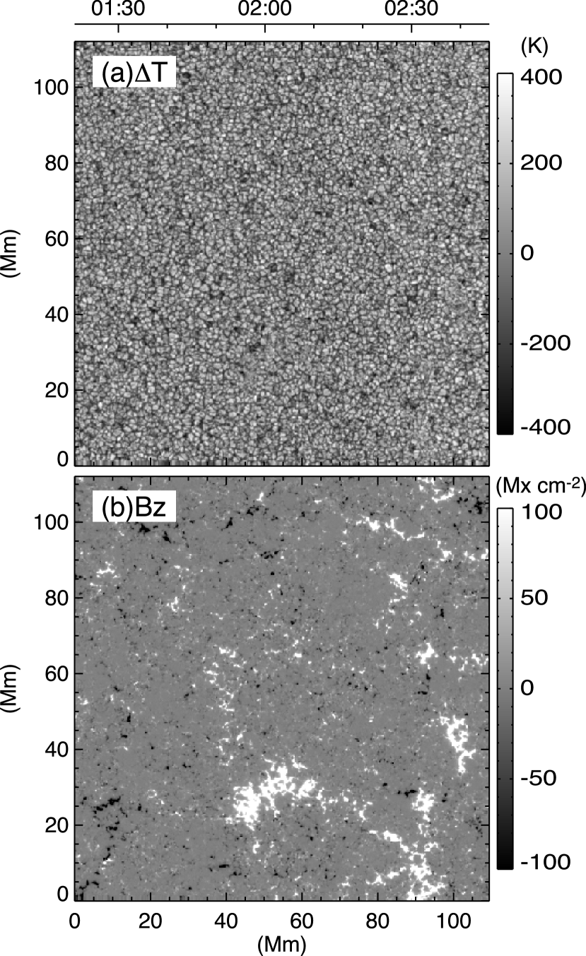
Figure 1.— Two dimensional maps of (a) the temperature fluctuation $\Delta T$ and (b) the vertical component of magnetic flux densities $B_{z}$ obtained with the Hinode SP on 24 April 2007, as an example of the data set used in the power spectrum analysis. The FOV is 1000 steps in the scanning direction and 1024 pixels along the slit, which covers a square of about 110 Mm. The hours of the SP scanning observation are shown at the top of the figure.

We use a data set taken with the SP of the Hinode SOT. The data set consists of 30 SP scans taken between November 2006 and December 2007. The SP recorded full Stokes spectra of the two Fe I lines at 630.15 nm and 630.25 nm with the normal map mode whose spatial sampling was about 0.15” per pixel and integration time is 4.8 sec per slit position. The field-of-views (FOVs) of the scans were equal to or more than 1000 steps in the scanning direction and 1024 pixels along the slit, and containing the solar disk center. It took about 85 minutes to complete the scan of each FOV. Their observing targets were mostly in quiet regions, but some of the scans included active regions also. We identify 23 scans out of 30 containing only the quiet regions using the condition in which an averaged density of unsigned flux $\left<|Bz|\right>$ in the FOV is smaller than 20 Mx cm^-2. The SP data are calibrated with the standard routine sp_prep available under the Solar SoftWare (SSW). The wavelength positions of the two Fe I lines are calibrated with an average line-center position outside of a sunspot.

The SP data provide two-dimensional maps of surface temperatures, line-of- sight (LOS) velocities, and magnetic field vectors. The temperatures $T$ are obtained using continuum intensities averaged in the spectral window outside of the Fe I lines and under assumption of black body radiations. We assume that average temperature $T_{0}$ is 6520 K outside of sunspots to convert the observed continuum intensities to the temperature. The LOS velocities $v_{z}$ are obtained using Doppler shifts of the Fe I line at 630.15 nm. The magnetic field vectors $(B_{x},B_{y},B_{z})$ are determined from wavelength-integrated Zeeman-induced polarization signals with the method described in Lites et al. (2008). The x, y, and z components correspond to ones in the scanning, slit, and line-of-sight directions, respectively. It is not necessary to convert the observed vectors into the ones in the local reference frame because the maps were taken near the disk center. To derive the transverse component $(B_{x},B_{y})$, the 180 degrees ambiguity in the azimuth angle has to be resolved. This is simply done by choosing the azimuth to be closest to the computed potential field using $B_{z}$ as an input. Fig. 1 shows two dimensional maps of the temperature fluctuation $\Delta T=T-T_{0}$ and the vertical component of magnetic flux densities $B_{z}$ as an example of the data set.

2.2. Derivation of power spectra

For deriving spatial power spectra, we apply the two-dimensional Fourier-transform to each map of the above parameters,

$$P(f;k_{x},k_{y})=\left|\frac{1}{N^{2}}\sum_{x,y}f(x,y)\exp\left(-2\pi i(k_{x}x+k_{y}y)\right)\right|^{2},$$ (1)

where $f(x,y)$ is either $\Delta T=T-T_{0}$, $v_{z}$, $B_{x}$, $B_{y}$, or $B_{z}$, and $N$ the number of pixels in one direction and 1024 in our analysis. The wavenumbers in the x and y directions are represented as $k_{x}$ and $k_{y}$. To have 1024 pixels in both the x(scanning)- and y(slit)- directions for simplifying the Fourier-transform in Eq. (1), we extract 1024 steps closest to the disk center when the number of steps in a scan is more than 1024. Because our selection criteria of the SP data set is that the number of pixels in the x-direction is more than 1000, the number of pixels in the x-direction is fewer than 1024 pixels in some of the maps. For those maps, we apply padding at both the ends in the x-direction to make a map consisting of $1024\times 1024$ pixels. We confirmed that the influence of the edges and padding is negligible when we apply a Hamming window in the Fourier-transform.

The two dimensional spatial power spectra $P(f;k_{x},k_{y})$ is then converted to their one dimensional form $P(f;k)$ by integrating the two-dimensional power spectrum in azimuthal angle of the wavenumber $(k_{x},k_{y})$,

$$P(f;k)=2\pi k\left<P(f;k_{x},k_{y})\right>_{k^{\prime}\in[k-\Delta k/2,k+\Delta k/2)},$$ (2)

where $k^{\prime}=\sqrt{k_{x}^{2}+k_{y}^{2}}$, and $\Delta k$ is the sampling interval of the wavenumber, $\Delta k=1/(N\Delta x)$, where $\Delta x$ is the pixel scale and 0.15” or 0.11 Mm on the solar surface. The power spectra thus derived are normalized using the following equations to represent them in a unit of energy density per unit wavenumber, erg cm^-3 (1/Mm)^-1,

$$E_{th}(k) = \frac{3}{2}\frac{nk_{B}}{T_{0}}\frac{P(\Delta T;k)}{\Delta k}$$ (3)

$$E_{vz}(k) = \frac{1}{2}\rho\frac{P(v_{z};k)}{\Delta k}$$ (4)

$$E_{bh}(k) = \frac{1}{8\pi}\frac{\left(P(B_{x};k)+P(B_{y};k)\right)}{\Delta k}$$ (5)

$$E_{bz}(k) = \frac{1}{8\pi}\frac{P(B_{z};k)}{\Delta k},$$ (6)

respectively, where $k_{B}$ is the Boltzman constant, $n$ the number density on the solar surface, where we assume $n=1\times 10^{17}$ cm^-3 as a typical photospheric number density, $\rho$ the mass density on the solar surface, where we assume $\rho=2.7\times 10^{-7}$ g cm^-3. The method used here is essentially consistent with the ones used in previous studies (such as Rieutord et al. 2010) except the normalization. The power spectra $E_{th}(k)$, $E_{vz}(k)$, $E_{bh}(k)$, and $E_{bz}(k)$ are created from each map. The power spectra averaged in the quiet regions (i. e. using 23 maps out of 30) are shown as dashed curves in Fig. 2.

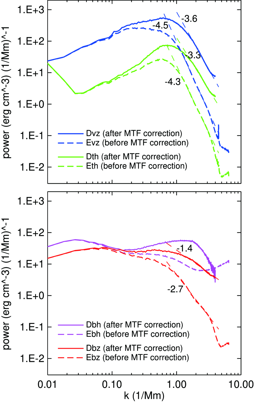
Figure 2.— Spatial power spectra of temperatures (green curves in the top panel), LOS velocities (blue curves in the top panel), and horizontal and vertical magnetic fields (purple and red curves in the bottom panel). The dashed and solid curves indicate power spectra before and after the instrument MTF and noise correction, respectively. The numbers indicate the power-law indices $\alpha$ obtained in the wavenumber range between $k=$ 1.5 and 3.5 Mm^-1.

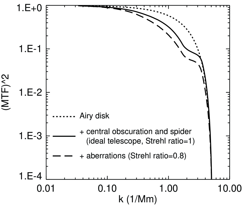
Figure 3.— Square of the Modulation Transfer Functions (MTFs) of the instrument at 630 nm. The dotted curve represents a square of MTF of an Airy disk of a 50 cm diameter aperture. The solid curve is for an ideal telescope without any aberrations (i.e. the Strehl ratio is unity), which includes the central obscuration and spiders. The dashed curve is for a telescope with some aberrations whose Strehl ratio is about 0.8.

Because the power in the higher wavenumber domain is affected by the instrumental spatial resolution, it is necessary to calibrate the optical transfer function to obtain the shape of the power spectra on the solar surface. The modulation transfer function (MTF) of the instrument is evaluated at 630 nm and is shown in Fig. 3. Though the telescope achieved diffraction limited performance (Suematsu et al. 2008; Wedemeyer-Böhm 2008), there are some residual aberrations in the optical performance. In this analysis, we use the MTF when the telescope has some aberration whose Strehl ratio is 0.8 (dashed curve in Fig. 3). The MTF is similar to the one used in Danilovic et al. (2008) who studied contrast of granules with Hinode SP data. Though the MTF falls down to zero at around $k=5$ Mm^-1 (corresponding to 200 km) as is shown in Fig. 3, the observed power spectra shown as dashed curves in Fig. 2 have significant power in the wavenumber range higher than 5 Mm^-1. The residual power in the high wavenumber range is mainly attributed to noises in the observed maps. The power due to the noises should be subtracted for calibrating the MTF, otherwise higher power appears erroneously in that range. When the data has a spatially uncorrelated white noise in a two-dimensional map, the noise spectrum $N_{f}(k)$ is expected to be proportional to $k$ in one-dimensional power spectra (see Rieutord et al. 2010). Thus the noise power $N_{f}(k)$ of each parameter is estimated using the linear regression of the power spectrum $E_{f}(k)$ in the wavenumber range between $k=$ 5 and 6 Mm^-1. MTF-calibrated power spectra $D_{f}(k)$ are then obtained using the following equation (see Lee et al. 1997);

$$D_{f}(k)=(E_{f}(k)-N_{f}(k))/MTF(k)^{2}.$$ (7)

The calibrated power spectra averaged in the quiet regions are shown as solid curves in Fig. 2, which show that the power in the wavenumber range higher than $k=0.1$ Mm^-1 is recovered by the calibration of the instrument MTF. The power in the wavenumber range higher than 4 Mm^-1 is acknowledged to be sensitive to how we subtract the noise power. Thus, the calibrated power spectra $D_{f}(k)$ are shown up to 4 Mm^-1 in Fig. 2.

3. Power spectra at the granular and supergranular scales

The SP FOVs used to make the power spectra are a square of about 110 Mm, which contain several supergranules whose typical diameters are 20 – 30 Mm, and make it possible to cover both the granular and supergranular scales. The thermal power spectrum $D_{th}(k)$ and the velocity power spectrum $D_{vz}(k)$ averaged in the quiet regions look very similar, as is shown in the top panel of Fig. 2. This can be naturally explained by the fact that there is a good correlation between the velocity and the intensity due to the thermal convection (e.g. Kirk & Livingston 1968; Beckers & Parnell 1969) at the granular scale. Both the power spectra have a peak at $k\sim 1$ Mm^-1, which corresponds to the spatial scale of about 1000 km and the granular scale. In the wavenumber range higher than the granular scale, i.e. in the spatial scale smaller than granules, the power spectra appear to be obeying the power-law (i. e. $\propto k^{\alpha}$). When we derive the power-law indices $\alpha$ of the power spectra between $k=$ 1.5 and 3.5 Mm^-1, the indices are -3.3 and -3.6 for $D_{th}(k)$ and $D_{vz}(k)$, respectively. Note that the power-law indices indicate that the slopes of the power spectra at the scale smaller than granules are significantly steeper than $k^{-5/3}$ which is predicted by the Kolmogorov’s law for isotropic turbulences. The power-law indices are much steeper than the ones in Müller (1989) and Espagnet et al. (1993) in which they reported that the slopes of the power spectra are close to Kolmogorov’s $k^{-5/3}$ power-law. Recent studies indicated power-law indices of about -3 based on a blue continuum image at 450 nm taken with the broadband filter imager (BFI) of Hinode SOT (Rieutord et al. 2010) and about -4 based on a broadband image taken through a TiO filter at 705.7 nm with the New Solar Telescope (NST) of Big Bear Solar Observatory (BBSO) (Goode et al. 2010), which are not so different from our results.

On the other hand, the power spectra do not show any enhancements in the lower wavenumber domain at 0.03 – 0.05 Mm^-1 corresponding to the supergranular scale. This is expected because vertical flows associated with supergranulation are slower than 50 m s^-1 (Hathaway et al. 2002) on the surface, and is more than one order of magnitude smaller than vertical flows of granulation, while horizontal flows of supergranulation are 300 – 500 m s^-1 (Simon & Leighton 1964; Orozco Suárez et al. 2012) and are known to make a peak in power spectra at the supergranulation scale (Hathaway et al. 2000; Rieutord et al. 2010).

The magnetic power spectra $D_{bz}(k)$ and $D_{bh}(k)$ shown in the bottom panel in Fig. 2 are completely different from $D_{th}(k)$ and $D_{vz}(k)$. Both the horizontal and vertical powers distribute over a broad wavenumber range. There are weak enhancements at the granular scale ($k\sim$ 1 Mm^-1) and at the supergranular scale ($k\sim$ 0.03 – 0.05 Mm^-1), in both $D_{bz}(k)$ and $D_{bh}(k)$, which suggests that the granular and supergranular scales are typical ones characterizing the magnetic field distribution on the solar surface. As we mentioned above, there are no significant powers at the supergranular scale in the spectra of the vertical velocities. But it is expected that the power of the horizontal velocities are strong enough to make the magnetic field structures, network fields, at the supergranular scale (Orozco Suárez et al. 2012). Note that there are no clear enhancements of the power around the proposed mesogranular scale $k\sim$ 0.1 – 0.4 Mm^-1, corresponding to 2.5 – 10 Mm, (November et al. 1981; Chou et al. 1992) in all the power spectra shown in Fig. 2, which is consistent with Hathaway et al. (2000) and Rieutord et al. (2010). There are some residual magnetic powers in the intermediate scale between the granular and supergranular scales. Ishikawa & Tsuneta (2010) suggested that sporadic appearance of granular-scale horizontal magnetic fields preferentially happens around boundaries of mesogranules (see also Yelles Chaouche et al. 2011). Such mesogranular-scale magnetic structures might be related with the residual magnetic power in the intermediate scale, though we need careful analysis including horizontal velocities that we cannot obtain only with the SP data.

In the wavenumber range higher than the granular scale, the slopes of the magnetic power spectra are clearly less steep than the power spectra of the thermal power $D_{th}(k)$ and the velocity power $D_{vz}(k)$. The power-law index $\alpha$ of $D_{bz}(k)$ is $-1.4$ in the wavenumber range between $k=$ 1.5 and 3.5 Mm^-1 though it is hard to say that the power spectrum obeys the power-law only from this analysis. The horizontal magnetic power spectrum $D_{bh}(k)$ has its peak at 1.3 – 2 Mm^-1 corresponding to 500 – 800 km, which is slightly smaller than the granular scale seen in $D_{vz}(k)$ and $D_{th}(k)$. The spatial scale of the magnetic spectra is in agreement with the observed size of transient horizontal magnetic fields (Ishikawa & Tsuneta 2009b). The slope of $D_{bh}(k)$ looks steeper than that of $D_{bz}(k)$ though we have to take into account relatively larger noises in the horizontal magnetic power. We will look into this in the next section.

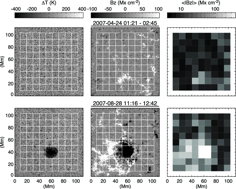
Figure 4.— Sub-regions used in the power spectrum analysis in Section 4 are shown on Hinode SP maps of the temperature fluctuation $\Delta T$ (left panels) and the vertical component of magnetic flux densities $B_{z}$ (middle panels). Each sub-region consists of $96\times 96$ pixels corresponding to a square of about 10 Mm. An average unsigned flux density $\left<|B_{z}|\right>$ is calculated in each sub-region as shown in the right panels. The top panels show maps obtained on 24 April 2007 which contain only a quiet region in the FOV. The bottom panels show maps obtained on 28 August 2007 which contain an active region in the FOV. We do not use the regions near the boundary of the SP maps and sub-regions containing a sunspot in this analysis. These regions are shown as blank areas in the $\left<|B_{z}|\right>$ maps (right panels).

4. Dependence of the power spectra on the unsigned magnetic flux density

4.1. Power spectra in small FOVs

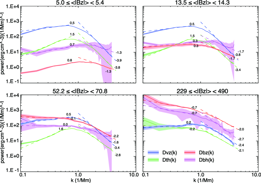
Figure 5.— Power spectra $D_{th}(k)$ (green curves), $D_{vz}(k)$ (blue curves), $D_{bz}(k)$ (red curves), and $D_{bh}(k)$ (purple curves) made in the sub-regions of the SP maps. Here shown are the spectra averaged in the intervals of 5.0 Mx cm^-2 $\leq\left<|B_{z}|\right><$ 5.4 Mx cm^-2 (top left), 13.5 Mx cm^-2 $\leq\left<|B_{z}|\right><$ 14.3 Mx cm^-2 (top right), 52.2 Mx cm^-2 $\leq\left<|B_{z}|\right><$ 70.8 Mx cm^-2 (bottom left), 229 Mx cm^-2 $\leq\left<|B_{z}|\right><$ 490 Mx cm^-2 (bottom right). The shaded area of each power spectrum represents the $\pm 1\sigma$ range showing variation of the power spectra in each interval of $\left<|B_{z}|\right>$. The values in the plots indicate the power-law indices $\alpha$ obtained between $k=$ 0.15 and 0.6 Mm^-1 and between $k=$ 1.8 and 3.2 Mm^-1.

The power spectra shown in the previous section were obtained in the quiet regions, thus including both internetwork and network regions. In this section, we analyze power spectra separately in internetwork and network regions. To do this, each SP map is divided into $9\times 9$ sub-regions whose FOVs are $96\times 96$ pixels, corresponding to a square of about 10 Mm, as is shown in Fig. 4. The FOVs of the sub-regions are not enough to cover the supergranular scale, but are enough to include many granules. The sub-regions are extracted not to use pixels near the edges of the SP maps. A power spectrum is obtained in each sub-region, using the same method described in §2 except the number of pixels in one direction $N$. The noise subtraction and the MTF correction are also applied to the power spectrum in each sub-region. An averaged density of unsigned flux $\left<|B_{z}|\right>$ is calculated in each sub-region, as is shown in the right panels of Fig. 4. The power spectra obtained in the sub-regions are averaged when they have similar $\left<|B_{z}|\right>$. The interval of $\left<|B_{z}|\right>$ for averaging the power spectra is determined to have 50 sub-regions in each interval. All the 30 SP maps are used in this analysis. Some of the sub-regions include sunspots in their FOVs, but such sub-regions are not used by checking $\left<|B_{z}|\right>$.

Fig. 5 shows the thermal, kinetic, and magnetic power spectra obtained in the sub-regions. The power spectra are the ones averaged in the interval of 5.0 Mx cm^-2 $\leq\left<|B_{z}|\right><$ 5.4 Mx cm^-2, corresponding to weak internetwork regions, 13.5 Mx cm^-2 $\leq\left<|B_{z}|\right><$ 14.3 Mx cm^-2, corresponding to strong internetwork regions, 52.2 Mx cm^-2 $\leq\left<|B_{z}|\right><$ 70.8 Mx cm^-2, corresponding to network regions, and 229 Mx cm^-2 $\leq\left<|B_{z}|\right><$ 490 Mx cm^-2, corresponding to strong network and plage regions. The shaded area of each power spectrum shows variation of the power spectra ($\pm 1\sigma$) in each interval. It is obvious that the magnetic power spectra of the horizontal component $D_{bh}(k)$ have large variations, which is due to relatively weaker signals in the linear polarization. The power spectra are shown in the wavenumber range up to $k=3.9$ Mm^-1 because the power in the higher wavenumber range tends to be affected by the noise subtraction.

Neither thermal or kinetic power spectra, $D_{th}(k)$ and $D_{vz}(k)$, change much when the average unsigned flux density is weaker than 20 Mx cm^-2 in the internetwork regions (top two panels in Fig. 5). There are peaks at around $k\sim 1$ Mm^-1 corresponding to the granular scale. In the wavenumber range higher than $k=1$ Mm^-1, i.e. in the spatial scale smaller than granules, the power-law indices are steeper than -3 in the wavenumber range between $k=$ 1.8 and 3.2 Mm^-1. The results are more or less consistent with the power spectra obtained in §3. On the other hand, the magnetic power spectra clearly varies depending on the average unsigned flux density $\left<|B_{z}|\right>$. When the average flux density is very small (top left in Fig. 5), the shapes of the power spectra look similar between $D_{bh}(k)$ and $D_{bz}(k)$. Both the spectra have peaks at around $k\sim 1.3$ Mm^-1 corresponding to about 800 km, which is slightly smaller than the granular scale and comparable with the observed size of horizontal magnetic field structures, as mentioned in the previous section. Orozco Suárez & Katsukawa (2012) examined distribution of magnetic field inclinations in internetwork regions at different heliocentric angles, and concluded that the inclination distribution partly resulted from the granular-scale loop-like magnetic features. The observed peak in the magnetic power spectra shown in Fig. 5 probably corresponds to such loop-like features, which are important constituents of the internetwork magnetic fields. The horizontal magnetic power $D_{bh}(k)$ is also acknowledged to be larger than the vertical one $D_{bz}(k)$ in the internetwork regions (top two panels in Fig. 5). This result looks consistent with Lites et al. (2008) where they reported predominance of apparent horizontal flux in internetwork regions. The power-law indices are around $-1.3$ for both the vertical and horizontal magnetic power spectra in the wavenumber range between $k=$ 1.8 and 3.2 Mm^-1. Similar power-law indices of the magnetic power spectra were reported in previous studies (Lee et al. 1997; Abramenko et al. 2001) although they were based on magnetic power spectra at the spatial scale larger than granules. Our magnetic power spectra show positive slopes at that scale in the internetwork regions. Stenflo (2012) showed that a magnetic power spectrum obtained with a Hinode SP data set exhibited a slope that was described by a power-law whose index was about $-3.2$ for spatial scales smaller than 1.2 Mm. The above power-law index was derived from the power spectrum without applying calibration of the instrument MTF. In our analysis, the raw magnetic power spectrum before applying the MTF calibration is about $-2.7$, as is shown in the bottom panel of Fig. 2, which is not so different from the one in Stenflo (2012).

When the average unsigned flux density is large in the network and plage regions (bottom panels in Fig. 5), the absolute vertical magnetic power increases. The increase in magnetic power is especially noticeable in the lower wavenumber range ($k<1$ Mm^-1). The horizontal magnetic power also exhibits similar behavior, and increases in the lower wavenumber range. The slope of the power $D_{bh}(k)$ and $D_{bz}(k)$ changes the sign from positive to negative in the wavenumber range lower than $k=1$ Mm^-1, which makes the peak at the granular scale less pronounced in the network regions. The thermal and kinetic power spectra become affected by the relatively strong magnetic fields in these regions. The kinetic power $D_{vz}(k)$ tends to decrease at the granular scale $k\sim 1$ Mm^-1, which is naturally explained by suppression of the convective motion by magnetic fields. It is also realized that the kinetic and thermal powers tend to be slightly enhanced in the wavenumber range higher than 2 Mm^-1. The increase in thermal and kinetic power at the small scale can be attributed to contributions of faculae structures created by small-scale magnetic fields. The suppression of the convection at the granular scale and the enhancements of the small-scale power makes the power spectra $D_{th}(k)$ and $D_{vz}(k)$ less steep in the wavenumber range higher than $k=1$ Mm^-1. Surprisingly, all the thermal, kinetic, and magnetic power spectra show similar slopes in the wavenumber range higher than $k=1$ Mm^-1 when the average unsigned flux density is bigger than 200 Mx cm^-2 (bottom right panel in Fig. 5).

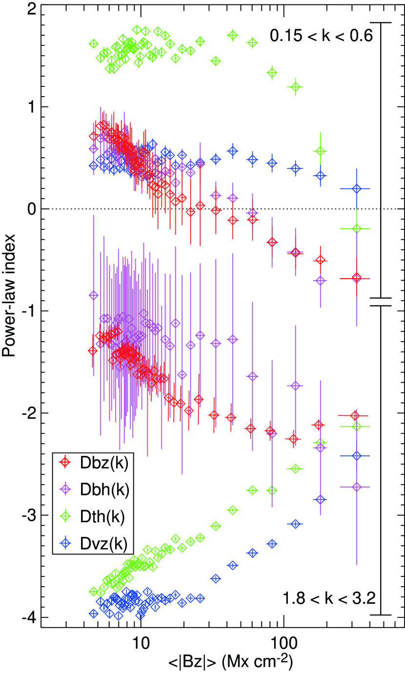
Figure 6.— Power-law indices $\alpha$ of the power spectra as a function of the averaged density of unsigned flux $\left<|B_{z}|\right>$. The power law indices are obtained in the two wavenumber ranges, between $k=$0.15 and 0.6 Mm^-1 (corresponding to the scale larger than granules) and between $k=$1.8 and 3.2 Mm^-1 (corresponding to the scale smaller than granules). The green, blue, red, and purple symbols represent the power-lawn indices of $D_{th}(k)$, $D_{bz}(k)$, $D_{bz}(k)$, and $D_{bh}(k)$, respectively. The vertical error bars show $\pm 1\sigma$ range of the power-law indices when we take into account the variation of the power spectra in each $\left<|B_{z}|\right>$ interval.

4.2. Dependence of the power-law indices on the unsigned magnetic flux density

Here we derive the power-law indices $\alpha$ of the power spectra obtained in the sub-regions. The power spectra used here are averaged ones in the interval of $\left<|B_{z}|\right>$, as described in the previous subsection. Thus we can get the power-law indices $\alpha$ as a function of $\left<|B_{z}|\right>$. Because the power spectra have different slopes between $k<1$ Mm^-1 (larger than the granular scale) and $k>1$ Mm^-1 (smaller than the granular scale), we derive the power-law indices $\alpha$ separately in these two wavenumber ranges. Here we use the wavenumber range between $k=$ 0.15 and 0.6 Mm^-1 and $k=$ 1.8 and 3.2 Mm^-1. We do not say that the power spectra follow the power-law in these wavenumber ranges, but the indices are used to characterize the slope of the power spectra. The variation of the power spectra in each $\left<|B_{z}|\right>$ interval is taken into account, and is reflected in errors of the power-law indices.

Fig. 6 displays the power-law indices $\alpha$ as a function of the averaged unsigned flux density $\left<|B_{z}|\right>$. Power-law indices of the thermal and kinetic power spectra $D_{th}(k)$ and $D_{vz}(k)$ change similarly as a function of $\left<|B_{z}|\right>$, while those of vertical and horizontal magnetic power spectra $D_{bz}(k)$ and $D_{bh}(k)$ behave similarly as well within the error bars. When the unsigned flux density is smaller than around $20$ Mx cm^-2, the difference of the power-law indices is significant between the magnetic power spectra and the thermal/kinetic ones in the higher wavenumber range (smaller than the granular scale). The latter power spectra are steeper than the former ones, and the power-law indices differ by about 2. The magnetic and thermal/kinetic power spectra tend to have similar slopes when the unsigned flux density becomes large. All the power-law indices are around -2 when the average unsigned flux density is bigger than 200 Mx cm^-2.

In the smaller wavenumber range (larger than the granular scale), the power-law indices of the magnetic power-spectra decrease monotonically with the unsigned flux density $\left<|B_{z}|\right>$, as is shown in the upper part of Fig. 6. They change the sign from positive to negative when $\left<|B_{z}|\right>$ is 20 – 50 Mx cm^-2. The power-law indices of the thermal and kinetic power spectra do not change so much when $\left<|B_{z}|\right>$ is smaller than around 100 Mx cm^-2, and they decrease when $\left<|B_{z}|\right>$ is bigger than around 100 Mx cm^-2. The positive slopes become almost zero or negative when $\left<|B_{z}|\right>$ is around 300 Mx cm^-2, which means that the peaks at the granular scale disappear in the thermal and kinetic power spectra. When we extrapolate the trend to the larger flux, the power-law indices in the smaller and larger wavenumber ranges might become similar. This suggests that the power spectra might be represented as a single slope in such large magnetic fluxes, though this is out of the scope of this article.

5. Summary and Discussion

We showed the power spectral analysis of the thermal, kinetic, and magnetic structures on the solar surface with the data set taken with the Hinode SP, including calibration of the instrumental effects. We showed in §3 that the kinetic and thermal power spectra had a peak at the granular scale while the magnetic power spectra had a broadly distributed power in various spatial scales, but had two weak peaks at both the granular and supergranular scales. We did not find enhancements of the magnetic power at the mesogranular scale though there were residual powers in between the granular and supergranular peaks. In §4 the power spectral analysis was done in the small sub-regions to distinguish the internetwork and network regions. We examined the slopes of the power spectra using the power-law indices, and compared them with the unsigned magnetic flux density averaged in the sub-regions. In the wavenumber range higher than $k=1$ Mm^-1, the thermal and kinetic power spectra exhibited steeper slopes than the magnetic ones in the internetwork regions, and the power-law indices differed by about 2. The slopes of the thermal and kinetic power spectra became less steep when the unsigned flux density increased, and the power-law indices of all the thermal, kinetic, and magnetic power spectra became similar.

In the internetwork regions, where the averaged density of the unsigned flux is very small, magnetic field structures are passively advected by the convective motion. According to Moffatt (1961), when the magnetic field is proportional to $(\nabla\cdot{\bf v})$ or $(\nabla\times{\bf v})$ in such weak field regions, its power spectrum is expected to vary as $D_{b}(k)\propto k^{2}D_{v}(k)$, where $D_{b}(k)$ and $D_{v}(k)$ are magnetic and kinetic power spectra including all the three components. This relationship predicts that the slope of the magnetic power spectrum is less steep than the kinetic one, and the difference of the power-law indices is 2, which is consistent with the observed difference of the power-law indices in the higher wavenumber range ($k>1$ Mm^-1) in the internetwork regions. In this analysis, we could not obtain the kinetic power spectrum in all the three components, but only in the vertical component. We need the horizontal velocity components to fully justify the scenario. When the unsigned flux is large, the magnetic structures are no longer passive to the convective motion. In this regime, magnetic and velocity fields strongly interact with each other, which possibly produces similar slopes between the magnetic power spectrum and the kinetic one.

The total magnetic energy is provided by integration of the power spectra in the wavenumber domain, $\int_{k_{0}}^{k_{1}}\left[D_{bz}(k)+D_{bh}(k)\right]dk$, where $k_{0}$ and $k_{1}$ are the lower and upper ends of the wavenumber range for the integration. When both the power spectra are represented as a power-law ($\propto k^{\alpha}$), the total magnetic energy is completely different in the case of between $\alpha<-1$ and $\alpha>-1$. When $\alpha<-1$ (steeper than $k^{-1}$), the total magnetic energy mainly comes from the power at the lower wavenumber, $D_{bz}(k_{0})+D_{bh}(k_{0})$. On the other hand, the total magnetic energy mainly comes from the power at the upper wavenumber, $D_{bz}(k_{1})+D_{bh}(k_{1})$, when $\alpha>-1$ (less steep than $k^{-1}$). The power-law indices of the magnetic power spectra obtained in the internetwork regions are close to or smaller than $-1$ in the wavenumber range higher than $k=1$ Mm^-1. This means that the total magnetic energy mainly comes from either the granular-scale ($k\sim 1$ Mm^-1) magnetic structures or both the granular-scale and smaller ones contributing evenly.

Recent numerical simulations of the surface magneto-convection suggested that turbulent fields were created by small-scale dynamo action, and a significant amount of unsigned flux was not detected at the spatial resolution of the Hinode SP because of cancellation of polarization signals from opposite magnetic polarities (Vögler & Schüssler 2007; Pietarila Graham et al. 2009, 2010). These numerical simulations indicated positive slopes of the magnetic power spectra toward the small scales even at the spatial scale smaller than granules. The slopes do not agree with the magnetic power spectra presented in this article. If we extrapolate the observed slope $k^{-1.3}$ of the magnetic power spectra up to $50$ Mm^-1, an order of magnitude higher than the Hinode SP resolution, the magnetic power in the observed wavenumber range between 1 and 4 Mm^-1 is about 50 % of the power between 1 and 50 Mm^-1, which is not as small as the percentage suggested by Pietarila Graham et al. (2009). Because we cannot argue behavior of the power spectra in unresolved scales based on these data, it is critical to use high-resolution data to extend the current analysis toward such small scales. Goode et al. (2010) and Abramenko et al. (2012) showed kinetic power spectra of transverse velocities down to the 0.1 Mm scale based on high-resolution imaging data taken with the 1.6 meter NST of BBSO, but they did not have magnetic field measurements yet. One possibility is to use magnetogram data taken with the Imaging Magnetograph eXperiment (IMaX) on board the 1 meter Sunrise balloon-borne observatory (Martínez Pillet et al. 2011) to extend the power spectra down to the 0.1 Mm scale. Stenflo (2012) argued possible existence of a flux tube population at the spatial scale close to or smaller than the resolution limit of the Hinode SP using a deep mode data set. Because the subtraction of the noise spectrum becomes critical to derive the power in the higher wavenumber range, we could not argue the power at the spatial scale below 0.25 Mm using the normal mode data in this article. It is important to use polarimetric data with a higher signal-to-noise ratio for studying the power at the spatial scale as close as the instrumental resolution limit.

References

- Abramenko & Yurchyshyn (2010) Abramenko, V., & Yurchyshyn, V. 2010, ApJ, 720, 717
- Abramenko et al. (2012) Abramenko, V., Yurchyshyn, V., & Goode, P. R. 2012, in Astronomical Society of the Pacific Conference Series, Vol. 455, 4th Hinode Science Meeting: Unsolved Problems and Recent Insights, ed. L. Rubio, F. Reale, & M. Carlsson, 17
- Abramenko et al. (2001) Abramenko, V., Yurchyshyn, V., Wang, H., & Goode, P. R. 2001, Sol. Phys., 201, 225
- Abramenko (2005) Abramenko, V. I. 2005, ApJ, 629, 1141
- Beckers & Parnell (1969) Beckers, J. M., & Parnell, R. L. 1969, Sol. Phys., 9, 39
- Chou et al. (1992) Chou, D.-Y., Chen, C.-S., Ou, K.-T., & Wang, C.-C. 1992, ApJ, 396, 333
- Danilovic et al. (2008) Danilovic, S., Gandorfer, A., Lagg, A., Schüssler, M., Solanki, S. K., Vögler, A., Katsukawa, Y., & Tsuneta, S. 2008, A&A, 484, L17
- Danilovic et al. (2010) Danilovic, S., Schüssler, M., & Solanki, S. K. 2010, A&A, 513, A1+
- Durrant & Nesis (1982) Durrant, C. J., & Nesis, A. 1982, A&A, 111, 272
- Espagnet et al. (1993) Espagnet, O., Muller, R., Roudier, T., & Mein, N. 1993, A&A, 271, 589
- Frenkiel & Schwarzschild (1955) Frenkiel, F. N., & Schwarzschild, M. 1955, ApJ, 121, 216
- Goode et al. (2010) Goode, P. R., Yurchyshyn, V., Cao, W., Abramenko, V., Andic, A., Ahn, K., & Chae, J. 2010, ApJ, 714, L31
- Hathaway et al. (2000) Hathaway, D. H., Beck, J. G., Bogart, R. S., Bachmann, K. T., Khatri, G., Petitto, J. M., Han, S., & Raymond, J. 2000, Sol. Phys., 193, 299
- Hathaway et al. (2002) Hathaway, D. H., Beck, J. G., Han, S., & Raymond, J. 2002, Sol. Phys., 205, 25
- Ichimoto et al. (2008) Ichimoto, K., et al. 2008, Sol. Phys., 249, 233
- Ishikawa & Tsuneta (2009a) Ishikawa, R., & Tsuneta, S. 2009a, A&A, 495, 607
- Ishikawa & Tsuneta (2009b) Ishikawa, R., & Tsuneta, S. 2009b, in Astronomical Society of the Pacific Conference Series, Vol. 415, The Second Hinode Science Meeting: Beyond Discovery-Toward Understanding, ed. B. Lites, M. Cheung, T. Magara, J. Mariska, & K. Reeves, 132
- Ishikawa & Tsuneta (2010) —. 2010, ApJ, 718, L171
- Kirk & Livingston (1968) Kirk, J. G., & Livingston, W. 1968, Sol. Phys., 3, 510
- Knobloch & Rosner (1981) Knobloch, E., & Rosner, R. 1981, ApJ, 247, 300
- Kosugi et al. (2007) Kosugi, T., et al. 2007, Sol. Phys., 243, 3
- Lee et al. (1997) Lee, J., Chae, J., Yun, H. S., & Zirin, H. 1997, Sol. Phys., 171, 269
- Lites (2011) Lites, B. W. 2011, ApJ, 737, 52
- Lites et al. (2008) Lites, B. W., et al. 2008, ApJ, 672, 1237
- Martínez Pillet et al. (2011) Martínez Pillet, V., et al. 2011, Sol. Phys., 268, 57
- Moffatt (1961) Moffatt, K. 1961, Journal of Fluid Mechanics, 11, 625
- Müller (1989) Müller, R. 1989, in NATO ASIC Proc. 263: Solar and Stellar Granulation, ed. R. J. Rutten & G. Severino, 101
- Nakagawa & Levine (1974) Nakagawa, Y., & Levine, R. H. 1974, ApJ, 190, 441
- Nakagawa & Priest (1973) Nakagawa, Y., & Priest, E. R. 1973, ApJ, 179, 949
- November et al. (1981) November, L. J., Toomre, J., Gebbie, K. B., & Simon, G. W. 1981, ApJ, 245, L123
- Orozco Suárez & Katsukawa (2012) Orozco Suárez, D., & Katsukawa, Y. 2012, ApJ, 746, 182
- Orozco Suárez et al. (2012) Orozco Suárez, D., Katsukawa, Y., & Bellot Rubio, L. R. 2012, ApJ, submitted
- Petrovay (2001) Petrovay, K. 2001, Space Sci. Rev., 95, 9
- Pietarila Graham et al. (2010) Pietarila Graham, J., Cameron, R., & Schüssler, M. 2010, ApJ, 714, 1606
- Pietarila Graham et al. (2009) Pietarila Graham, J., Danilovic, S., & Schüssler, M. 2009, ApJ, 693, 1728
- Reiling (1971) Reiling, H. 1971, Sol. Phys., 19, 297
- Rieutord & Rincon (2010) Rieutord, M., & Rincon, F. 2010, Living Reviews in Solar Physics, 7, 2
- Rieutord et al. (2010) Rieutord, M., Roudier, T., Rincon, F., Malherbe, J., Meunier, N., Berger, T., & Frank, Z. 2010, A&A, 512, A4+
- Roudier et al. (1991) Roudier, T., Vigneau, J., Espagnet, O., Muller, R., Mein, P., & Malherbe, J. M. 1991, A&A, 248, 245
- Shimizu et al. (2008) Shimizu, T., et al. 2008, Sol. Phys., 249, 221
- Simon & Leighton (1964) Simon, G. W., & Leighton, R. B. 1964, ApJ, 140, 1120
- Stenflo (2012) Stenflo, J. O. 2012, A&A, 541, A17
- Suematsu et al. (2008) Suematsu, Y., et al. 2008, Sol. Phys., 249, 197
- Tsuneta et al. (2008) Tsuneta, S., et al. 2008, Sol. Phys., 249, 167
- Vögler & Schüssler (2007) Vögler, A., & Schüssler, M. 2007, A&A, 465, L43
- Wedemeyer-Böhm (2008) Wedemeyer-Böhm, S. 2008, A&A, 487, 399
- Yelles Chaouche et al. (2011) Yelles Chaouche, L., et al. 2011, ApJ, 727, L30