Measuring topology in a laser-coupled honeycomb lattice:
From Chern insulators to topological semi-metals

Abstract

Ultracold fermions trapped in a honeycomb optical lattice constitute a versatile setup to experimentally realize the Haldane model [Phys. Rev. Lett. 61, 2015 (1988)]. In this system, a non-uniform synthetic magnetic flux can be engineered through laser-induced methods, explicitly breaking time-reversal symmetry. This potentially opens a bulk gap in the energy spectrum, which is associated with a non-trivial topological order, i.e., a non-zero Chern number. In this work, we consider the possibility of producing and identifying such a robust Chern insulator in the laser-coupled honeycomb lattice. We explore a large parameter space spanned by experimentally controllable parameters and obtain a variety of phase diagrams, clearly identifying the accessible topologically non-trivial regimes. We discuss the signatures of Chern insulators in cold-atom systems, considering available detection methods. We also highlight the existence of topological semi-metals in this system, which are gapless phases characterized by non-zero winding numbers, not present in Haldane’s original model.

1 Introduction

Topological phases of matter have been a topic of great interest in condensed matter physics since the discovery of the integer quantum Hall effect [vonKlitzing:1986]. They are characterized by transport properties – such as a quantized Hall conductivity – that depend on the topological structure of the eigenstates [Kohmoto:1985], and not on the details of the microscopic Hamiltonian. As a result, such properties are remarkably robust against external perturbations. Integer quantum Hall phases, the first topological insulating phases to be discovered [vonKlitzing:1986], are realized by applying a large uniform magnetic field to a quasi-ideal two-dimensional electron gas, as formed in layered semiconductors structures.

The presence of a uniform magnetic field is not, however, a necessary condition to produce quantum Hall states, as first realized by Haldane [Haldane1988]. He proposed a remarkably simple model on a honeycomb lattice, with real nearest-neighbor (NN) hopping and complex next-nearest neighbor (NNN) hopping mimicking the Peierls phases experienced by charged particles in a magnetic field. Although the magnetic flux through an elementary cell of the honeycomb lattice is zero, a staggered magnetic field present within this cell locally breaks time-reversal symmetry. Haldane showed that this model supports phases that are equivalent to integer quantum Hall phases: they correspond to insulators with quantized Hall conductivities, $\sigma_{H}=\nu\,e^{2}/h$ where $e$ is the electron charge. In this manner, it is possible to generate a quantum Hall effect without a uniform external magnetic field. The integer $\nu=\pm 1$ (depending on the particular values of the microscopic parameters) is a topological invariant – the Chern number – characteristic of the phase and robust with respect to small perturbations [Thouless1982, Kohmoto:1985]. More recently, a more broad concept of topological insulators has emerged, classifying all possible topological phases for non-interacting fermions in terms of their symmetries [Hasan2010, Qi2011]. In this modern terminology, the Haldane model belongs to the class A of Chern insulators, which are topologically equivalent to the standard quantum Hall states.

The Haldane model has not been directly realized in solid-state systems, due to the somewhat artificial structure of the staggered magnetic field. Interestingly, ultracold atomic gases [Lewenstein:2007, Bloch2008a] appear better suited to achieve this goal [Liu:2010, Stanescu:2010]. In recent years, many proposals have been put forward to realize artificial magnetic fields for ultracold atoms (see [Dalibard2011] for a review). Staggered fields are relatively easier to implement than uniform ones [Jaksch2003, Gerbier2010, Lim2008], and have already been realized in a square optical lattice [aidelsburger2011]. Building on these ideas, Alba and coworkers [Alba2011] proposed a model very similar to Haldane’s that could be realized with ultracold atoms. Their variant is based upon a state-dependent honeycomb optical lattice [Bloch2008a], where cold atoms in two different internal “pseudospin” states are localized at two inequivalent sites of the elementary cell. Additionally, laser induced transitions [Jaksch2003, Ruostekoski:2002] between the nearest-neighbor sites lead to pseudospin-dependent hopping matrix elements containing phase factors, schematically depicted in Fig. 1. Furthermore, Alba and coworkers [Alba2011] suggested a measurement based on spin-resolved time-of-flight (ToF) experiments to identify topological invariants.

The present work provides a systematic analysis of the model proposed in Ref. [Alba2011] and identifies parameter regimes where Chern insulators emerge. The goals are: firstly, to serve as a detailed guide to possible experiments aiming at realizing such topological phases; and secondly, to discuss the subtle issue of identifying them through ToF methods. Ref.  [Alba2011] focused on the very special case when one of the NNN hopping amplitudes was zero, and we find that such a system is semi-metallic, not a quantized Chern insulator. In this limit, where the bulk energy gap is closed, the Hall conductivity is no longer simply given by a Chern number $\sigma_{H}\neq\nu\,e^{2}/h$, and therefore, this transport coefficient generally looses its topological stability. Yet, the ToF method seems to give a non-trivial signature in this regime, which is robust with respect to small variations of model parameters. The subtlety is that the ToF method of Ref. [Alba2011] actually measures a winding number [Qi:2006], which only coincides with a topologically protected Hall conductivity when the energy gap is open. If this condition is met, the ToF method of Ref. [Alba2011] then produces a reasonable experimental measure of the topologically invariant Chern number, and we indeed verify its robustness when varying the system parameters. Interestingly, if the bulk gap is closed, we find that the winding number measured from a ToF absorption image might still depict a stable plateau when varying the microscopic parameters, under the condition that the Fermi energy is exactly tuned at the gap closing point. In this work, such gapless phases associated with a non-trivial winding number will be referred to as topological semi-metals. Absent in the original Haldane model, they constitute intriguing topological phases, which can be created and detected in the laser-coupled honeycomb lattice.

In this work, several types of band structures and topological orders will therefore be present: (1) Chern insulating phases, i.e. gapped phases with non-trivial Chern numbers $\nu=\pm 1$, (2) Topological semi-metals, i.e. gapless phases associated with a non-trivial winding number, (3) Standard semi-metals, i.e. gapless phases with the two bands touching at the Dirac points, as in graphene [Wallace1947, CastroNeto2009], and which are found at the transition between two topological phases.

This paper is structured as follows. In Sect. 2, we introduce the model and discuss how the energy band topology can be characterized in terms of Chern numbers. We also discuss the magnetic flux configuration as a function of the model parameters, highlighting the time-reversal-symmetry breaking regimes. Sect. LABEL:topologicalphases presents the main results, where the phase diagrams are investigated as a function of the microscopic parameters. In Sect. LABEL:skyrmion, we examine the signatures of the ToF method [Alba2011], and compare its results when applied to a Chern insulator or to a semi-metallic phase, i.e., when the topological bulk gap is absent. We summarize the results in Sect. LABEL:conclusions, and discuss an extension which implements the Kane-Mele model leading to $\mathbb{Z}_{2}$ topological insulators [Kane:2005].

2 The Model and the gauge structure

2.1 The Hamiltonian

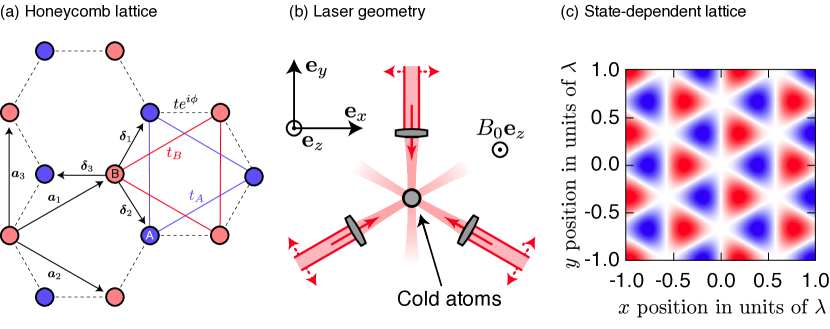
Figure 1: (a) Honeycomb lattice composed of two coupled triangular sublattices $A$ and $B$. The site positions in each sublattice are defined as $\boldsymbol{r}_{m_{A}}=m_{1}\boldsymbol{a}_{1}+m_{2}\boldsymbol{a}_{2}$ and $\boldsymbol{r}_{m_{B}}=m_{1}\boldsymbol{a}_{1}+m_{2}\boldsymbol{a}_{2}-\boldsymbol{\delta}_{2}$, with unit vectors $\boldsymbol{a}_{1}=\boldsymbol{\delta}_{1}-\boldsymbol{\delta}_{3}$ and $\boldsymbol{a}_{2}=\boldsymbol{\delta}_{2}-\boldsymbol{\delta}_{3}$ and with $m=(m_{1},m_{2})$ integer. The nearest-neighbour vectors are $\boldsymbol{\delta}_{1}=a/2(1,\sqrt{3})$, $\boldsymbol{\delta}_{2}=a/2(1,-\sqrt{3})$ and $\boldsymbol{\delta}_{3}=a(-1,0)$. We define $\boldsymbol{a}_{3}=\boldsymbol{a}_{1}-\boldsymbol{a}_{2}=\boldsymbol{\delta}_{1}-\boldsymbol{\delta}_{2}$. The hopping factors between NN and NNN sites of the honeycomb lattice are indicated by $t_{A}$, $t_{B}$ and $te^{i\phi}$, with $\phi\equiv\phi(m_{A},m_{B})$ given by Eq. peierls. The lattice spacing is $a\sqrt{3}$, and we set $a=1$ in the main text, which defines our unit of length. (b) Three-beam laser configuration giving rise to the desired spin-dependent hexagonal lattice, which we describe for ${}^{40}K$. In this vision, the lasers are detuned between the D1 and D2 lines of the 4S-4P transition, whereby the state-independent (scalar) light shift is zero. The remaining spin-dependent potential – an effective Zeeman magnetic field – is depicted in (c). The strength of the “same-spin” hopping, i.e. $t_{a}$ and $t_{b}$, is governed by the choice of internal states: the pair $\left|f=9/2,m_{F}=7/2\right>$ and $\left|f=7/2,m_{F}=7/2\right>$ produce $t_{a}\approx t_{b}$ as they have opposite magnetic moments. In contrast, the choice $\left|f=9/2,m_{F}=9/2\right>$ and $\left|f=7/2,m_{F}=7/2\right>$ produces $t_{a}\neq t_{b}$. The effective Zeeman shift is plotted with a color scale where blue indicates the potential minima for pseudo-spin up atoms, forming the A sublattice; and red indicates the minima for pseudo-spin down atoms, forming the B sublattice. Not shown are an additional pair of Raman lasers, also in the ${\bf e}_{x}\!-\!{\bf e}_{y}$ plane, that couple between the different sublattices (red and blue in (c)).

In the model introduced in Ref. [Alba2011], cold fermionic atoms are trapped in a honeycomb structure formed by two intertwined triangular optical lattices, whose sites are labeled by $A$ and $B$ respectively [cf. Fig. 1 (a)-(c)]. In the tight-binding regime – applicable for sufficiently deep optical potentials $V_{A,B}(\boldsymbol{x})$ – atoms are only allowed to hop between neighboring sites of the two triangular sublattices, which correspond to next-nearest neighbors of the honeycomb lattice (denoted $\langle\langle n_{\tau},m_{\tau}\rangle\rangle$, with $\tau=A,B$). The second-quantized Hamiltonian takes the form

$$\hat{H}_{\text{NNN}}=-t_{A}\sum_{\langle\langle n_{A},m_{A}\rangle\rangle}\hat{a}^{\dagger}_{n_{A}}\hat{a}_{m_{A}}-t_{B}\sum_{\langle\langle n_{B},m_{B}\rangle\rangle}\hat{b}^{\dagger}_{n_{B}}\hat{b}_{m_{B}},$$ (1)

where $\hat{a}_{m_{A}}$ ($\hat{b}_{m_{B}}$) is the field operator for annihilation of an atom at the lattice site $\boldsymbol{r}_{m_{A}}$ ($\boldsymbol{r}_{m_{B}}$) associated with the $A$ ($B$) sublattice, and where $t_{A,B}$ are the tunneling amplitudes. Furthermore, the two sublattices are coupled through laser-assisted tunneling, where hopping is induced between neighboring sites of the honeycomb lattice by a laser coupling the two internal states associated with each sublattice. This corresponds to tunneling processes linking nearest neighbors sites of the honeycomb lattice, denoted as $\langle m_{A},m_{B}\rangle$, which are described by the Hamiltonian

$$\hat{H}_{\text{NN}}=-t\sum_{\langle m_{A},m_{B}\rangle}\left(e^{i\phi(m_{A},m_{B})}\hat{a}^{\dagger}_{m_{A}}\hat{b}_{m_{B}}+h.\,c.\right).$$ (2)

Here, the phases $\phi(m_{A},m_{B})$ generated by the laser fields are the analogs of the Peierls phases familiar from condensed matter physics [Luttinger1951, Hofstadter1976], with $\boldsymbol{r}_{m_{A}}$ and $\boldsymbol{r}_{m_{B}}$ specifying the nearest neighboring sites of the hexagonal lattice. Following the approach of Jaksch and Zoller [Jaksch2003], these phases can be expressed in terms of the momentum $\boldsymbol{p}$ transferred by the laser-assisted tunneling as

$$\phi(m_{A},m_{B})=\boldsymbol{p}\cdot(\boldsymbol{r}_{m_{A}}+\boldsymbol{r}_{m_{B}})/2=-\phi(m_{B},m_{A}),$$ (3)

so that the phases have opposite signs for $\boldsymbol{r}_{A}\rightarrow\boldsymbol{r}_{B}$ and $\boldsymbol{r}_{B}\rightarrow\boldsymbol{r}_{A}$ hoppings (cf. Fig. LABEL:figfluxlattice(a) and Refs. [Dalibard2011, Gerbier2010]). Finally, the model also features an on-site staggered potential, described by

$$\hat{H}_{\text{stag}}=-\varepsilon\sum_{m}\left(\hat{a}^{\dagger}_{m_{A}}\hat{a}_{m_{A}}-\hat{b}^{\dagger}_{m_{B}}\hat{b}_{m_{B}}\right),$$ (4)

which explicitly breaks the inversion symmetry of the honeycomb lattice [Haldane1988]. The total Hamiltonian, given by

$$\hat{H}_{\text{tot}}=\hat{H}_{\text{NN}}+\hat{H}_{\text{NNN}}+\hat{H}_{\text{stag}},$$ (5)

is characterized by the hopping amplitudes ($t$, $t_{A}$ and $t_{B}$), the momentum transfer $\boldsymbol{p}=(p_{x},p_{y})$, as well as the mismatch energy $\varepsilon$.

To eliminate the explicit spatial dependence of our Hamiltonian htot, we perform the unitary transformation &^a^†_m_A →~a^†_m_A=^a^†_m_A exp(i p⋅r_m_A /2 ),
^b^†_m_B →~b^†_m_B=^b^†_m_B exp(- i p⋅r_m_B /2 ), giving a transformed Hamiltonian ^H_tot=& - t ∑_⟨n_A, m_B ⟩ ( ~a^†_n_A ~b_m_B + ~b^†_m_B ~a_n_A )
- t_A ∑_⟨⟨n_A, m_A ⟩⟩ e^i ~ϕ(n_A, m_A) ~a^†_n_A ~a_m_A - t_B ∑_⟨⟨n_B, m_B ⟩⟩ e^i ~ϕ(n_B, m_B) ~b^†_n_B ~b_m_B
- ε∑_m ( ~a^†_m_A ~a_m_A - ~b^†_m_B ~b_m_B ), with new Peierls phases given by &~ϕ(n_A, m_A)= p⋅(r_m_A - r_n_A)/2,
~ϕ(n_B, m_B)= p⋅(r_n_B - r_m_B)/2. The transformed Hamiltonian hamnew, featuring complex hopping terms along the links connecting NNN sites, is similar to the Haldane model [Haldane1988], but with important differences highlighted in Sect. LABEL:haldanesection.

Since $\boldsymbol{r}_{n_{A,B}}-\boldsymbol{r}_{m_{A,B}}=\boldsymbol{\delta}_{\mu}-\boldsymbol{\delta}_{\nu}=\pm\boldsymbol{a}_{\lambda}$ are the primitive lattice vectors of the honeycomb lattice (see Fig. 1), where $\mu,\nu,\lambda=1,2,3$, the phases $\tilde{\phi}$ in Eq. peierls2 no longer depend on the spatial coordinates. Therefore, the Hamiltonian hamnew is invariant under discrete translations, $[\hat{H}_{\text{tot}},\mathcal{T}_{1,2}]=0$ where $\mathcal{T}_{1,2}\psi(\boldsymbol{r})=\psi(\boldsymbol{r}+\boldsymbol{a}_{1,2})$, allowing us to invoke Bloch’s theorem and reduce the analysis to a unit cell formed by two inequivalent sites $A$ and $B$. In momentum space, the Hamiltonian takes the form of a $2\times 2$ matrix,

$$H(\boldsymbol{k})=-\pmatrix{\varepsilon}+2t_{A}f(\boldsymbol{k}-\boldsymbol{p}/2)&tg(\boldsymbol{k})\\ tg^{*}(\boldsymbol{k})-\varepsilon+2t_{B}f(\boldsymbol{k}+\boldsymbol{p}/2),$$ (6)

where &f (k)=∑_ν=1^3cos( k ⋅a_ν ),  g (k)=∑_ν=1^3 exp(-i k ⋅δ_ν), and $\boldsymbol{k}=(k_{x},k_{y})$ belongs to the first Brillouin zone (FBZ) of the system. We rewrite this Hamiltonian in the standard form

$$H(\boldsymbol{k})=\epsilon(\boldsymbol{k})\hat{1}+\boldsymbol{d}(\boldsymbol{k})\cdot\boldsymbol{\hat{\sigma}},$$ (7)

with

$$\epsilon(\boldsymbol{k})=-t_{A}f(\boldsymbol{k}-\boldsymbol{p}/2)-t_{B}f(\boldsymbol{k}+\boldsymbol{p}/2),$$ (8)

where $\boldsymbol{\hat{\sigma}}$ is the vector of Pauli matrices, and $\boldsymbol{d}(\boldsymbol{k})$ has real-valued Cartesian components defined by &d_x (k)-id_y (k)= - t g(k),
d