Solution of a model for the two-channel electronic Mach-Zehnder interferometer

Abstract

We develop the theory of electronic Mach-Zehnder interferometers built from quantum Hall edge states at Landau level filling factor $\nu=2$, which have been investigated in a series of recent experiments and theoretical studies. We show that a detailed treatment of dephasing and non-equlibrium transport is made possible by using bosonization combined with refermionization to study a model in which interactions between electrons are short-range. In particular, this approach allows a non-perturbative treatment of electron tunneling at the quantum point contacts that act as beam-splitters. We find an exact analytic expression at arbitrary tunneling strength for the differential conductance of an interferometer with arms of equal length, and obtain numerically exact results for an interferometer with unequal arms. We compare these results with previous perturbative and approximate ones, and with observations.

I Introduction

Electronic Mach-Zehnder interferometers (MZIs) built from quantum Hall edge states have attracted a great deal of recent interest, particularly because it has been found that they show striking non-equilibrium behaviour.Heiblum1 ; Heiblum2 ; litvin07 ; roulleau07 ; neder07 ; heiblum3 ; litvin08 ; roulleau08 ; RoulleauThese ; Roulleau ; roulleau09 ; bieri08 ; litvin2010 In these mesoscopic devices, quantum Hall (QH) edge states form the arms of an interferometer, joined at two points by quantum point contacts (QPCs) that serve as beam-splitters. Aharonov-Bohm (AB) oscillations in the differential conductance of the device are observedHeiblum1 as either the applied magnetic field or the length of one of the interferometer arms is varied. Effects out of equilibrium are probed by studying the visibility of AB oscillations as a function of bias voltage: remarkably, the visibility does not decrease monotonically with bias, but rather shows a sequence of ‘lobes’ separated by zeros or deep minima.Heiblum2

While theoretical workearly-theory investigating decoherence in electronic MZIs predates these experiments, the problem of understanding the origin of the observed lobe pattern has provided a fresh focus for such efforts.Cheianov ; ChGV ; Sukhorukov ; levk ; neder08 ; sim08 ; Kovrizhin1 ; Mirlin Starting from a description of edge states as one-dimensional interacting chiral conductors,halperin ; wen two main alternatives have emerged. One Sukhorukov is that the phenomenon is specific to Landau level filling factor $\nu=2$, and arises because in this case there are two types of collective modes wen with different velocities. The other,neder08 ; sim08 ; Kovrizhin1 worked out for $\nu=1$, is that the phenomenon is due to multiparticle interference effects and requires finite-range, rather than contact interactions.

In this paper we set out an approach that yields exact results for a model of an MZI at $\nu=2$ with contact interactions and arbitrary QPC tunneling probabilities, offering a test of previous perturbative Sukhorukov and approximate Mirlin calculations. Our approach circumvents a serious technical obstacle in the study of QH edge states coupled by QPCs, which is that interactions are most easily handled using bosonization,VonDelftSchoeller ; Giamarchi but this transformation converts the tunneling Hamiltonian from a one-body operator in fermionic coordinates to a non-linear (cosine) form in bosonic coordinates. Weak tunneling (or tunneling probability close to one) can then be treated perturbatively,Cheianov ; ChGV ; Sukhorukov but additional ideas are necessary in order to study the situation realised in most experiments, with tunneling probabilities close to one half. Two ways around this difficulty have been discussed previously. OneKovrizhin1 provides numerically exact results, but for simplified models in which electrons interact only when they are inside the interferometer. The otherMirlin can be applied to a general model of electron interactions, but has so far been implemented within an approximation scheme. The complementary route we describe here combines bosonization with refermionisationFabrizio ; vonDelft to arrive (for the simplest case of equal-length interferometer arms) at a transformed set of fermion creation and annihilation operators, in terms of which the full MZI Hamiltonian is quadratic. Similar methods were used recently by two of usKovrizhin2 to treat the related problempierre2010 ; quench2009 of equilibration in a QH edge state, downstream from a single biased QPC.

Our main result is that there are important differences between the behaviour of a model for an MZI at $\nu=2$ with only contact interactions and what has been observed experimentally. Some of these differences are already apparent in behaviour at weak tunneling, computed in Ref. Sukhorukov, . In particular for an interferometer with arms of equal length, which is the intended situation in most experiments, the visibility of interference fringes is not suppressed at large bias voltage. One might have hoped that the differences would be reduced or removed outside the weak-tunneling limit, but we show this is not the case. We conclude that, while models with contact interactions show oscillations of fringe visibility with bias voltage, they are not sufficient even outside the weak tunnelling limit to explain the envelope of the observed ‘lobe pattern’; instead allowance must be made for an additional ingredient (see Ref. Sukhorukov, for some possibilities). We note, in contrast, that both oscillations and a decaying envelope can arise from finite-range interactions, as discussed in Refs. neder08, ; sim08, ; Kovrizhin1, ; Mirlin, .

The remainder of the paper is organised as follows. In Section II we define the model we study for the electronic MZI, and in Section III we set out the bosonization and refermionisation transformations that we use. We give analytical results for interferometers with arms of equal length in Section IV, and describe our approach to interferometers with arms of different lengths in Section V, presenting numerical results for this case in Section VI. Finally, in Section VII we discuss our results in relation to past theoretical work and experimental observations. The numerical procedure used in evaluating the correlators is outlined in Appendix A, and some comparisons with perturbation theory are given in Appendix B.

II The model

We consider the model of an electronic Mach-Zehnder interferometer that is illustrated in Fig. 1. The MZI operates in the $\nu=2$ QH regime and is constructed from two quantum Hall edges labelled by an index $\eta=1,2$. Each of these edges carries two chiral electron channels with spin labels $s=\uparrow,\downarrow$. Two quantum point contacts $a$ and $b$, with positions separated by distance $d_{1}$ on the edge $1$ and $d_{2}$ on edge 2, induce electron tunnelling between channels 1$\downarrow$ and 2$\downarrow$. Two other channels, 1$\uparrow$ and 2$\uparrow$, are coupled to the rest of the system via contact interactions. This model was studied using a perturbative treatment of tunnelling in Ref. Sukhorukov, , and approximately for general tunnelling probabilities in Ref. Mirlin, .

The Hamiltonian $\hat{H}$ of the model can be written as

$$\hat{H}=\hat{H}_{\mathrm{0}}+\hat{H}_{\mathrm{tun}},$$ (1)

where $\hat{H}_{\mathrm{0}}$ represents the separate edges and $\hat{H}_{\mathrm{tun}}$ describes the tunnelling contacts. Defining fermionic fields $\hat{\psi}_{\eta s}^{\dagger}(x)$ that create an electron at position $x$ of the channel $\eta s$, with standard anticommutation relations

$$\{\hat{\psi}_{\eta s}(x),\hat{\psi}_{\eta^{\prime}s^{\prime}}^{\dagger}(x^{\prime})\}=\delta_{\eta\eta^{\prime}}\delta_{ss^{\prime}}\delta(x-x^{\prime}),$$ (2)

and introducing electron density operators

$$\hat{\rho}_{\eta s}(x)=\hat{\psi}_{\eta s}^{\dagger}(x)\hat{\psi}_{\eta s}(x),$$ (3)

the edge Hamiltonian (as originally proposed by Wen wen ) is

$$\hat{H}_{0}=-i\hbar v_{f}\sum_{\eta,s}\int\hat{\psi}_{\eta s}^{\dagger}(x)\partial_{x}\hat{\psi}_{\eta s}(x)dx\\ +2\pi\hbar g\sum_{\eta}\int\hat{\rho}_{\eta\uparrow}(x)\hat{\rho}_{\eta\downarrow}(x)dx.$$ (4)

Here, $g$ is the strength of short-range interactions between electrons with different spins on the same edge, and short-range intra-channel interactions have been absorbed into the definition of the Fermi velocity $v_{f}$.

Figure 1: Schematic view of the model of an electronic MZI treated in this paper. The interferometer is constructed from two QH edges, 1 and 2, each carrying two electron channels, $\uparrow$ and $\downarrow$. Horizontal arrows indicate the direction of electron motion in the channels. The channels 1$\downarrow$ and 2$\downarrow$ are connected via two QPCs, shown using dashed lines. Under single-channel bias, as in the experiments of Ref.  Heiblum2, , the channel 1$\downarrow$ is fed from a source at chemical potential $\mu_{1\downarrow}=eV$, and other channels have sources at $\mu_{\eta s}=0$. Under two-channel bias, as in the experiments of Ref. bieri08, , sources for the two channels 1$\uparrow$ and 1$\downarrow$ have $\mu_{1\uparrow}=\mu_{1\downarrow}=eV$, and the other two channels have sources at $\mu_{\eta s}=0$.

The tunnelling Hamiltonian $\hat{H}_{\mathrm{tun}}=\hat{H}_{\mathrm{tun}}^{a}+\hat{H}_{\mathrm{tun}}^{b}$ is characterised by the tunneling strengths $v_{a,b}$ and has the contributions

$$\hat{H}_{\mathrm{tun}}^{a} =v_{a}e^{i\alpha}\hat{\psi}_{1\downarrow}^{\dagger}(0)\hat{\psi}_{2\downarrow}(0)+\mathrm{h.c}.,$$ (5)

$$\hat{H}_{\mathrm{tun}}^{b} =v_{b}e^{i\beta}\hat{\psi}_{1\downarrow}^{\dagger}(d_{1})\hat{\psi}_{2\downarrow}(d_{2})+\mathrm{h.c}.,$$ (6)

where $\phi_{AB}=\beta-\alpha$ is the Aharonov–Bohm phase due to flux enclosed by the MZI.

A finite bias voltage is modelled by taking sources for different edge channels to have chemical potentials $eV$ and $0$ respectively. Two alternative bias schemes have been studied experimentally. In the first, which we refer to as single-channel bias (SCB), only the channel 1$\downarrow$ is at non-zero chemical potential, as in experiments of Ref. Heiblum2, . In the second, which we refer to as two-channel bias (TCB), both channels 1$\uparrow,$1$\downarrow$ are at the same non-zero chemical potential, as in the experiments of Ref. bieri08, . In calculations we establish a steady state for the interferometer by using the Hamiltonian $\hat{H}$ to time-evolve from the distant past an initial state $|{I}\rangle$ that is the ground state (or, at finite temperature, thermal equilibrium state) of $\hat{H}_{0}$ with the specified chemical potentials in each channel.

The edge Hamiltonian $\hat{H}_{\mathrm{0}}$ has a simple quadratic form after bosonization and the difficulties in computing time evolution arise from $\hat{H}_{\mathrm{tun}}$. For this it is convenient to use the interaction representation, taking the tunnelling Hamiltonian $\hat{H}_{\mathrm{tun}}$ as an “interaction” following Ref. ChGV, . The time dependence of operators in this representation, which we distinguish from the Schrödinger ones using an explicit time argument, is

$$\hat{A}(t)=e^{\frac{i}{\hbar}\hat{H}_{0}t}\hat{A}e^{-\frac{i}{\hbar}\hat{H}_{0}t}.$$ (7)

Similarly, evolution of the initial state from the distant past to time $t$ is induced by the operator

$$\hat{S}(t,-\infty)=\mathrm{T}\exp\left\{-\frac{i}{\hbar}\int_{-\infty}^{t}\hat{H}_{\mathrm{tun}}(\tau)\mathrm{d}\tau\right\}\,.$$ (8)

To obtain an expression for the current through the interferometer, we recall that the time-dependence of the total density on edge 2 is given (for $x\not=0,d_{2}$) by

$$\frac{i}{\hbar}\sum_{s}[\hat{H}_{0},\hat{\rho}_{2s}(x)]=-(v_{f}+g)\partial_{x}\sum_{s}\hat{\rho}_{2s}.$$ (9)

Using the continuity equation we can therefore take the current operator to be

$$\hat{I}=e(v_{f}+g)\sum_{s}\hat{\rho}_{2s}(x)\big{|}_{x_{1}}^{x_{2}}$$ (10)

where $x_{1}<0$ is any point before the MZI, $x_{2}>d_{2}$ is any point after the MZI, and $e$ is the electron charge. This definition is more convenient in our approach that the commonly-used alternative in terms of the rate of change of electron number on an edge. The steady-state current is then

$$I(V)=\langle I|\hat{S}^{\dagger}(0,-\infty)\hat{I}\hat{S}(0,-\infty)|I\rangle$$ (11)

where the bias voltage $V$ enters through the definition of $|I\rangle$. An important characteristic of electronic MZIs which quantifies the coherence and is measured in experiments, is the visibility of Aharonov-Bohm oscillations. It can be expressed in terms of the differential conductance

$$\mathcal{G}(V)=\mathrm{d}I(V)/\mathrm{d}V,$$ (12)

as the ratio

$$\mathcal{V}(V)=\frac{\mathcal{G}_{\mathrm{max}}(V)-\mathcal{G}_{\mathrm{min}}(V)}{\mathcal{G}_{\mathrm{max}}(V)+\mathcal{G}_{\mathrm{min}}(V)}.$$ (13)

Here $\mathcal{G}_{\mathrm{max/\min}}$ is the maximum/minimum of the differential conductance as a function of AB-phase at a fixed bias voltage. Our main aim in this paper is to calculate the visibility at arbitrary bias voltage and QPC tunnelling strengths for the model of Eq. (1).

III Transformations

We use a sequence of transformations to calculate the current in the model for an MZI defined in the previous section. Our approach (building on earlier workKovrizhin1 ; Kovrizhin2 by two of us) combines a treatment of interactions using bosonization with a fermionic description of the tunneling at QPCs, and can be separated into three steps.

First, we bring the Hamiltonian $\hat{H}_{0}$ into quadratic form in a standard way using bosonization. Second, the resulting expression is diagonalised by a unitary rotation of bosonic fields, where interactions result in appearance of two different plasmon velocities. Third, we refermionize the full Hamiltonian $\hat{H}$ by inroducing new Klein factors. With our choice of refermionization transformation, the tunnelling term $\hat{H}_{\mathrm{tun}}^{a}$ at contact $a$ retains its noninteracting form, while $\hat{H}_{\mathrm{tun}}^{b}$ acquires an additional phase factor, which can be written in terms of electron counting operators. Interestingly, in the case of an interferometer with equal arm lengths ($d_{1}=d_{2}$) this phase factor vanishes, and the interacting problem reduces to a noninteracting one, allowing an elementary analytical treatment. For an interferometer with unequal arm lengths ($d_{1}\neq d_{2}$) we derive an expression for the current in a form suitable for a simple and efficient numerical evaluation, and we present the details of this approach together with the results. These results are for zero temperature, but the expression for current through the MZI that we give here are general and can be used to study the finite temperature case.

III.1 Bosonization

We start by introducing briefly notation for the bosonization procedure that we use (see Refs. VonDelftSchoeller, , Giamarchi, and Kovrizhin1, for more details). We consider initially edges of finite length $L$, so that momentum $q$ is quantized as $q=2\pi n/L,$ $n\in Z$, then take $L$ to infinity. Fermionic fields $\hat{\psi}_{\eta s}(x)$ are expressed in terms of bosonic fields $\hat{\phi}_{\eta s}(x)$ via the bosonization identity

$$\hat{\psi}_{\eta s}(x)=(2\pi a)^{-1/2}\hat{F}_{\eta s}e^{i\frac{2\pi}{L}\hat{N}_{\eta s}x}e^{-i\hat{\phi}_{\eta s}(x)},$$ (14)

where we have introduced Klein factors $\hat{F}_{\eta s}$, particle number operators $\hat{N}_{\eta s}$ and a short-distance cutoff $a$. Electron density operators are expressed in terms of the bosonic field as

$$\hat{\rho}_{\eta s}(x)=\hat{N}_{\eta s}/L-(2\pi)^{-1}\partial_{x}\hat{\phi}_{\eta s}(x).$$ (15)

Bosonic fields have the mode expansion

$$\hat{\phi}_{\eta s}(x)=-\sum_{q>0}(2\pi/qL)^{{1}/{2}}[\hat{b}_{\eta s}(q)e^{iqx}+\mathrm{h.c.}]e^{-qa/2},$$ (16)

where $\hat{b}_{\eta s}^{\dagger}(q)$ is a boson creation operator with momentum $q$, obeying standard commutation relations

$$[\hat{b}_{\eta s}(q),\hat{b}_{\eta^{\prime}s^{\prime}}^{\dagger}(p)]=\delta_{\eta\eta^{\prime}}\delta_{ss^{\prime}}\delta_{qp}.$$ (17)

From Eqs. (16) and (17) the commutation relations for the $\hat{\phi}_{\eta s}(x)$ operators are

$$[\hat{\phi}_{\eta s}(x),\partial_{y}\hat{\phi}_{\eta s}(y)]=-2\pi i\delta_{\eta\eta^{\prime}}\delta_{ss^{\prime}}\delta(x-y).$$ (18)

The mode expansion for the fermonic operator is

$$\hat{\psi}_{\eta s}(x)=\frac{1}{\sqrt{L}}\sum_{k}\hat{c}_{\eta s}(k)e^{ikx}$$ (19)

and bosonic operators can be expressed in terms of fermions via the operator identity

$$\hat{b}_{\eta s}^{\dagger}(q)=i(2\pi/qL)^{1/2}\sum_{k=-\infty}^{+\infty}\hat{c}_{\eta s}^{\dagger}(k+q)\hat{c}_{\eta s}(k).$$ (20)

The Klein factors, which add or remove electrons on a given channel, have the commutation relations

$$\{\hat{F}_{\eta s}^{\dagger},\hat{F}_{\eta^{\prime}s^{\prime}}\}=2\delta_{\eta\eta^{\prime}}\delta_{ss^{\prime}},\text{ \ }[\hat{N}_{\eta s},\hat{F}_{\eta^{\prime}s^{\prime}}]=-\delta_{\eta\eta^{\prime}}\delta_{ss^{\prime}}\hat{F}_{\eta s}.$$ (21)

Using this bosonization prescription, we express the edge-state Hamiltonian $\hat{H}_{0}$ as

$$\hat{H}_{0}=\frac{\hbar v_{f}}{2}\sum_{\eta s}\int\frac{dx}{2\pi}[\partial_{x}\hat{\phi}_{\eta s}]^{2}+g\hbar\sum_{\eta}\int\frac{dx}{2\pi}\partial_{x}\hat{\phi}_{\eta\uparrow}\partial_{x}\hat{\phi}_{\eta\downarrow}\\ +\frac{2\pi g\hbar}{L}\sum_{\eta}\hat{N}_{\eta\uparrow}\hat{N}_{\eta\downarrow}+\frac{2\pi}{L}\frac{\hbar v_{f}}{2}\sum_{\eta s}\hat{N}_{\eta s}(\hat{N}_{\eta s}+1).$$ (22)

Similarly we represent the tunnelling Hamiltonian in terms of new bosonic fields, obtaining for contact $a$

$$\hat{H}_{\mathrm{tun}}^{a}=(2\pi a)^{-1}v_{a}e^{i\alpha}\hat{F}_{1\downarrow}^{\dagger}\hat{F}_{2\downarrow}e^{i[\hat{\phi}_{1\downarrow}(0)-\hat{\phi}_{2\downarrow}(0)]}+\mathrm{h.c.}$$ (23)

and for contact $b$

$$\hat{H}_{\mathrm{tun}}^{b}=(2\pi a)^{-1}v_{b}e^{i\beta}\hat{F}_{1\downarrow}^{\dagger}\hat{F}_{2\downarrow}e^{i\frac{2\pi}{L}[\hat{N}_{2\downarrow}d_{2}-\hat{N}_{1\downarrow}d_{1}]}\\ \times e^{i[\hat{\phi}_{1\downarrow}(d_{1})-\hat{\phi}_{2\downarrow}(d_{2})]}+\mathrm{h.c.}$$ (24)

Here we have kept the finite contribution to the phase arising from the particle number operators and neglected terms of higher order in $1/L$, which vanish in the thermodynamic limit.

III.2 Diagonalisation of the Hamiltonian

The edge-state Hamiltonian $\hat{H}_{0}$ given in Eq. (22) is quadratic and can be diagonalizedwen ; Kovrizhin2 by a unitary rotation of the bosonic fields

$$(\hat{\chi}_{S_{+}}\leavevmode\nobreak\ \hat{\chi}_{A_{-}}\leavevmode\nobreak\ \hat{\chi}_{A_{+}}\leavevmode\nobreak\ \hat{\chi}_{S_{-}})^{T}=U(\hat{\phi}_{1\uparrow}\leavevmode\nobreak\ \hat{\phi}_{1\downarrow}\leavevmode\nobreak\ \hat{\phi}_{2\downarrow}\leavevmode\nobreak\ \hat{\phi}_{2\uparrow})^{T},$$ (25)

with the rotation matrix

$$U=\frac{1}{2}\left(\begin{array}[]{rrrr}1&1&1&1\\ 1&-1&1&-1\\ 1&1&-1&-1\\ 1&-1&-1&1\end{array}\right).$$ (26)

The transformation preserves bosonic commutation relations

$$[\hat{\chi}_{p\sigma}(x),\partial_{y}\hat{\chi}_{p^{\prime}\sigma^{\prime}}(y)]=-2\pi i\delta_{pp^{\prime}}\delta_{\sigma\sigma^{\prime}}\delta(x-y).$$ (27)

Particle number operators $\hat{N}_{\eta s}$ transform in the same way as bosonic fields, and we use the subscript values $p\sigma=A_{\pm},S_{\pm}$ to distinguish the new operators from the old ones.

In terms of the new operators, we obtain

$$\hat{H}_{0}=\sum_{p\sigma}\frac{\hbar v_{\sigma}}{2}\int\frac{dx}{2\pi}[\partial_{x}\hat{\chi}_{p\sigma}]^{2}\\ +\frac{2\pi}{L}\sum_{p\sigma}\frac{\hbar v_{\sigma}}{2}\hat{N}_{p\sigma}^{2}+\frac{2\pi}{L}\hbar v_{f}\hat{N}_{S+},$$ (28)

where we have introduced the velocities

$$v_{\pm}=v_{f}\pm g.$$ (29)

The Hamiltonian of Eq. (28) describes four plasmon modes, two propagating with velocity $v_{+}$ and two with $v_{-}$. The final term of Eq. (28) is a constant of motion of $\hat{H}$ and we omit it in the following.

III.3 Refermionization

We refermionize the Hamiltonian $\hat{H}$ by introducing new fermionic fields, expressed in terms of the four new species of bosons $\hat{\chi}_{p\sigma}(x),$ new Klein factors $\hat{F}_{p\sigma}$ and particle number operators $\hat{N}_{p\sigma}$ (again employing the subscript values $p\sigma=A_{\pm},S_{\pm}$ to identify the new operators). The bosonization identity for the new fields is

$$\hat{\Psi}_{p\sigma}(x)=(2\pi a/v_{\sigma})^{-1/2}\hat{F}_{p\sigma}e^{i\frac{2\pi}{L}\hat{N}_{p\sigma}x}e^{-i\hat{\chi}_{p\sigma}(x)}.$$ (30)

Note that for convenience we normalise to unit current, with

$$\{\hat{\Psi}_{p\sigma}^{\dagger}(x),\hat{\Psi}_{p^{\prime}\sigma^{\prime}}(x^{\prime})\}=v_{\sigma}\delta_{pp^{\prime}}\delta_{\sigma\sigma^{\prime}}\delta(x-x^{\prime}).$$ (31)

The new fermion operators have the mode expansion

$$\hat{\Psi}_{p\sigma}(x)=\int\frac{d\varepsilon}{2\pi\hbar}e^{\frac{i}{\hbar}\varepsilon x/v_{\sigma}}\hat{a}_{p\sigma}(\varepsilon),$$ (32)

where $\hat{a}_{p\sigma}(\varepsilon)$ obeys

$$\{\hat{a}_{p\sigma}(\varepsilon),\hat{a}_{p^{\prime}\sigma^{\prime}}^{\dagger}(\varepsilon^{\prime})\}=2\pi\hbar\delta_{pp^{\prime}}\delta_{\sigma\sigma^{\prime}}\delta(\varepsilon-\varepsilon^{\prime}).$$ (33)

The edge-state Hamiltonian now assumes the simple form

$$\hat{H}_{0}=-i\hbar\sum_{p\sigma}\int dx\ \hat{\Psi}_{p\sigma}^{\dagger}\partial_{x}\hat{\Psi}_{p\sigma}=\sum_{p\sigma}\int\frac{d\varepsilon}{2\pi\hbar}\leavevmode\nobreak\ \varepsilon\ \hat{a}_{p\sigma}^{\dagger}(\varepsilon)\hat{a}_{p\sigma}(\varepsilon).$$ (34)

From Eqns. (7) and (34) we obtain an expression for the fermionic fields in the interaction representation

$$\hat{\Psi}_{p\sigma}(x,t)=\int\frac{d\varepsilon}{2\pi\hbar}e^{-\frac{i}{\hbar}\varepsilon(t-x/v_{\sigma})}\hat{a}_{p\sigma}(\varepsilon).$$ (35)

The new Klein factors that enter Eq. (30) can be related to the old ones by comparing changes in $\hat{N}_{\eta s}$ and $\hat{N}_{p\sigma}$ generated by Klein factors in the old and new bases, as described in Refs. vonDelft, and Kovrizhin2, . An important technical point follows from the fact that a unit change in a single $\hat{N}_{p\sigma}$ in the new basis is equivalent to changes of one half in two $\hat{N}_{\eta s}$’s in the old basis. The gluing conditions necessary to relate the two Fock spaces have been discussed carefully in Ref. vonDelft, : in summary, one requires

$$(\hat{N}_{S_{+}},\hat{N}_{A_{-}},\hat{N}_{A_{+}},\hat{N}_{S_{-}})\in({\mathbb{Z}}+P/2)^{4}$$

and

$$\hat{N}_{S_{+}}\pm\hat{N}_{A_{-}}=(\hat{N}_{A_{+}}\pm\hat{N}_{S_{-}})\,{\rm mod}2\,,$$

where $P=0,1$, according to the parity of the total number of electrons. All states in the original fermion basis can be represented by states in the transformed basis that satisfy these conditions. Conversely, states in the new fermion basis that do not satisfy these conditions are unphysical. Naturally, $\hat{H}_{\rm tun}$ has no non-zero matrix elements linking the physical and unphysical sectors. Similarly, only bi-linears and not single Klein factors can be transformed between bases: the expressions

$$\hat{F}_{S_{-}}^{\dagger}\hat{F}_{A_{-}}^{\dagger} {=} \hat{F}_{1\uparrow}^{\dagger}\hat{F}_{1\downarrow},\quad\hat{F}_{S_{-}}\hat{F}_{A_{-}}^{\dagger}=\hat{F}_{2\downarrow}^{\dagger}\hat{F}_{2\uparrow},$$ (36)

$$\hat{F}_{S_{-}}^{\dagger}\hat{F}_{A_{+}}^{\dagger} = \hat{F}_{1\uparrow}^{\dagger}\hat{F}_{2\downarrow},\quad\hat{F}_{S_{+}}^{\dagger}\hat{F}_{A_{-}}^{\dagger}=\hat{F}_{1\uparrow}^{\dagger}\hat{F}_{2\downarrow}^{\dagger}$$ (37)

follow directly from the form of the transformation $U$. We use these to transform the combination of Klein factors that enters the tunnelling Hamiltonian, finding

$$\hat{F}_{1\downarrow}^{\dagger}\hat{F}_{2\downarrow}=\hat{F}_{1\downarrow}^{\dagger}\hat{F}_{1\uparrow}\hat{F}_{1\uparrow}^{\dagger}\hat{F}_{2\downarrow}=-\hat{F}_{A_{+}}^{\dagger}\hat{F}_{A_{-}}.$$ (38)

This gives an expression for the tunnelling Hamiltonian at contact $a$ in terms of the new Klein factors

$$\hat{H}_{\mathrm{tun}}^{a}=-(2\pi a)^{-1}v_{a}e^{i\alpha}\hat{F}_{A_{+}}^{\dagger}\hat{F}_{A_{-}}e^{i[\hat{\chi}_{A_{+}}(0)-\hat{\chi}_{A_{-}}(0)]}+\mathrm{h.c.}$$ (39)

The crucial property of the transformation of Eq. (26) is that it preserves the form of the tunnelling Hamiltonian at contact $a$, in the sense that $\pm i\hat{\chi}_{A\pm}$ appears in the exponent with unit coefficient. That makes it possible to use Eq. (30) together with Eq. (39) to obtain the tunnelling Hamiltonian in terms of new fermions, as

$$\hat{H}_{\mathrm{tun}}^{a} =\tilde{v}_{a}e^{i\alpha}\hat{\Psi}_{A_{+}}^{\dagger}(0)\hat{\Psi}_{A_{-}}(0)+\text{{h.c.}},$$ (40)

$$\hat{H}_{\mathrm{tun}}^{b} =\tilde{v}_{b}e^{i\beta}e^{i\pi\hat{Q}}\hat{\Psi}_{A_{+}}^{\dagger}(d_{1})\hat{\Psi}_{A_{-}}(d_{2})+\mathrm{h.c.},$$ (41)

where we have introduced renormalised tunnelling strengths

$$\tilde{v}_{a,b}=-v_{a,b}/\sqrt{v_{+}v_{-}}.$$ (42)

The phase operator $\hat{Q}$ is given by

$$\hat{Q} = \frac{2}{L}(\hat{N}_{2\downarrow}d_{2}-\hat{N}_{1\downarrow}d_{1}+\hat{N}_{A_{+}}d_{1}-\hat{N}_{A_{-}}d_{2})$$ (43)

$$+\frac{1}{\pi}[\hat{\phi}_{1\downarrow}(d_{1})-\hat{\phi}_{2\downarrow}(d_{2})-\hat{\chi}_{A_{+}}(d_{1})+\hat{\chi}_{A_{-}}(d_{2})]$$

$$= [\mathcal{\hat{N}}_{S+}-\mathcal{\hat{N}}_{S-}]-[\mathcal{\hat{N}}_{A+}+\mathcal{\hat{N}}_{A-}]$$

where

$$\hat{\mathcal{N}}_{p\sigma}=\int_{d_{1}}^{d_{2}}\mathrm{d}x\,\hat{\rho}_{p\sigma}(x)$$ (44)

Here density operators $\hat{\rho}_{p\sigma}(x)$ are defined in terms of the bosonic fields $\hat{\chi}_{p\sigma}(x)$ by analogy with Eq. (15). Eq. (44) shows that $\mathcal{\hat{N}}_{p\sigma}$ counts the number of particles passing the QPC $a$ during the time window $(-d_{2}/v_{\sigma},-d_{1}/v_{\sigma})$.

To find how an applied bias voltage is described in terms of the new fermions, note that the chemical potentials in each channel enter the grand canonical distribution in the combination $\sum_{\eta s}\mu_{\eta s}\hat{N}_{\eta s}$. The transformation between $\hat{N}_{\eta s}$ and $\hat{N}_{p\sigma}$ therefore implies that

$$(\mu_{S_{+}}\mu_{A_{-}}\mu_{A_{+}}\mu_{S-})^{T}=U^{-1}(\mu_{1\uparrow}\mu_{1\downarrow}\mu_{2\downarrow}\mu_{2\uparrow})^{T},$$ (45)

which leads to the results shown in Table 1. It is also interesting to consider explicitly how an initial state $|I\rangle$ appears in the two bases. In the vacuum for the system without tunnelling, in which all four channels are at zero chemical potential, all single particle eigenstates are filled with electrons from momentum $-\infty$ up to zero. Klein factors act on this Fermi sea by adding or removing particles. Consider as an example the case of two-channel bias, for which the initial state has equal chemical potentials in both spin channels. To reach this initial state from the vacuum we need to add equal numbers of electrons to each of the channels 1$\downarrow$ and 1$\uparrow$, which is achieved by acting repeatedly with the product of Klein factors $\hat{F}_{1\uparrow}^{\dagger}\hat{F}_{1\downarrow}^{\dagger}$. Since $\hat{F}_{1\uparrow}^{\dagger}\hat{F}_{1\downarrow}^{\dagger}=F_{A_{+}}^{\dagger}F_{S_{+}}^{\dagger}$, this state is also one with equal, non-zero particle number in channels $A_{+}$ and $S_{+}$ and zero particle number in the other channels.

	SCB	TCB
$\mu_{S_{+}}$	$+eV/2$	$eV$
$\mu_{S_{-}}$	$-eV/2$	$0$
$\mu_{A_{+}}$	$+eV/2$	$eV$
$\mu_{A_{-}}$	$-eV/2$	$0$

Table 1: Chemical potentials for the new fermions in the two experimental setups.

A final step is to re-write the current operator, Eq. (10), in terms of the new operators, as

$$\hat{I}=ev_{+}[\hat{\rho}_{S_{+}}(x)-\hat{\rho}_{A_{+}}(x)]\big{|}_{x=x_{1}}^{x=x_{2}}$$ (46)

Equations (34), (40) and (41) represent the central result of this paper. They give an exact mapping of the initial interacting problem to the one where the interaction effects have been absorbed into the phase shifts for electrons scattering at the QPC $b$. We note that although the channels $S_{\pm}$ are not coupled by tunnelling, they generate contributions to the phase operators. In the special case of an interferometer with equal arm lengths the phase operator $\hat{Q}$ vanishes and the full Hamiltonian $\hat{H}=\hat{H}_{0}+\hat{H}_{\mathrm{tun}}$ acquires the form for an MZI without interactions but with edges having two different Fermi velocities, $v_{+}$ and $v_{-}$.

IV Interferometer with equal arm lengths

We first discuss the behaviour of the interferometer in the special case of equal arm lengths, for which it is possible to obtain complete analytical results in a straightforward way. With $d_{1}=d_{2}\equiv d$, $\hat{H}_{\mathrm{tun}}$ retains a noninteracting form after refermionization. By an elementary calculation, scattering between the channels $A_{+}$ and $A_{-}$ at contact $a$ is described by the $S$-matrix

$$\mathcal{S}_{a}=\left(\begin{array}[]{cc}r_{a}&-ie^{i\alpha}t_{a}\\ -ie^{-i\alpha}t_{a}&r_{a}\end{array}\right)\,,$$ (47)

where the transmission and reflection amplitudes are $t_{a}=\sin(\tilde{v}_{a}/\hbar)\$and $r_{a}=\cos(\tilde{v}_{a}/\hbar)$. The simplification for an MZI with equal arm lengths is that scattering at QPC $b$ is represented in the same basis by an equivalent matrix $\mathcal{S}_{b}$.

To calculate current and hence visibility, consider a fermion incident on the interferometer in channel $A_{+}$ and exiting in the same channel. Two paths contribute to this process, with quantum-mechanical amplitudes $A_{(i)}$ and $A_{(ii)}$ as shown in Fig. 2. The amplitudes include distinct phase shifts for each path: the phase difference encodes interaction effects and is inversely proportional to

$$v_{\mathrm{eff}}=[1/v_{-}-1/v_{+}]^{-1}.$$

We use the form of the current operator given in Eq. (46). At an energy for which particles are incident in the channel $A_{+}$ but not in $A_{-}$, the occupation probability of outgoing states in $A_{+}$ is $|A_{(i)}+A_{(ii)}|^{2}$.

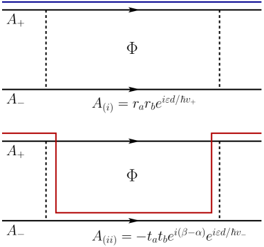
Figure 2: (Color online) Two paths through the interferometer with the corresponding amplitudes for a particle starting on the channel $A_{+}$ before the QPC $a$ and exiting in the same channel after QPC $b$. Channels $S_{\pm}$ are not shown.

We hence obtain for the current

$$I(V)=e\int\frac{d\varepsilon}{2\pi\hbar}\{1-|A_{(i)}+A_{(ii)}|^{2}\},$$ (48)

where the integral is taken from the chemical potential in channel $A_{-}$ to that in $A_{+}$. Defining the tunnelling and reflection probabilities $T_{a,b}=t_{a,b}^{2}$ and $R_{a,b}=r_{a,b}^{2}$ the integrand can be written

$$1-|A_{(i)}+A_{(ii)}|^{2} = R_{a}T_{b}+T_{a}R_{b}$$

$$+ 2(T_{a}T_{b}R_{a}R_{b})^{\frac{1}{2}}\cos({\phi_{AB}}+{\varepsilon d/\hbar v_{\mathrm{eff}}}).$$

Under single-channel bias the energy window for integration is from Table I $(-eV/2,eV/2)$. We find for the incoherent contribution

$$I_{0}=\frac{e^{2}V}{2\pi\hbar}[R_{a}T_{b}+T_{a}R_{b}],$$ (49)

and for the contribution sensitive to the phase $\phi_{AB}$

$$I_{AB}^{(\mathrm{SCB})}=e\int_{-eV/2}^{eV/2}\frac{d\varepsilon}{2\pi\hbar}2(T_{a}T_{b}R_{a}R_{b})^{\frac{1}{2}}\cos({\phi_{AB}}+{\varepsilon d/\hbar v_{\mathrm{eff}}}).$$ (50)

From these equations we obtain the conductance

$$\mathcal{G}^{(\mathrm{SCB})}=\frac{e^{2}}{2\pi\hbar}[R_{a}T_{b}+T_{a}R_{b}\\ +2(T_{a}T_{b}R_{a}R_{b})^{\frac{1}{2}}\cos(\phi_{V}/2)\cos\varphi_{AB}],$$ (51)

where $\phi_{V}=eVd/\hbar v_{\mathrm{eff}}$ is a voltage dependent phase shift which appears as a result of interactions. From Eq. (51) we find the visibility under single-channel bias

$$\mathcal{V}^{(\mathrm{SCB})}=\mathcal{V}_{0}|\cos(eVd/2\hbar v_{\mathrm{eff}})|,$$ (52)

where $\mathcal{V}_{0}$ is the visibility of a noninteracting two-paths MZI with a single biased channel

$$\mathcal{V}_{0}=\frac{2(T_{a}T_{b}R_{a}R_{b})^{\frac{1}{2}}}{R_{a}T_{b}+T_{a}R_{b}}.$$ (53)

We see that, with this bias arrangement, interactions generate an oscillatory behavior of the visibility as a function of bias voltage with the period inversely proportional to the interferometer arm length. This period diverges together with $v_{\mathrm{eff}}$ in the noninteracting limit. Similar behavior was found for an MZI with equal arm lengths using perturbation theory at small tunnelling in Ref. Sukhorukov, and from an approximate theory in Ref. Mirlin, . We stress that the result (52) we obtain is in fact an exact feature of the model.

Under two-channel bias the energy window for integration is $(0,eV)$ and we obtain for the coherent contribution to the current

$$I_{AB}^{(\mathrm{TCB})}=e\int_{0}^{eV}\frac{d\varepsilon}{2\pi\hbar}2(T_{a}T_{b}R_{a}R_{b})^{\frac{1}{2}}\cos({\phi_{AB}}+{\varepsilon d/\hbar v_{\mathrm{eff}}})$$ (54)

and for the conductance

$$\mathcal{G}^{(\mathrm{TCB})}=\frac{e^{2}}{2\pi\hbar}[R_{a}T_{b}+T_{a}R_{b}\\ +2(T_{a}T_{b}R_{a}R_{b})^{\frac{1}{2}}\cos(\phi_{AB}+\phi_{V})].$$ (55)

In this expression the voltage dependent phase shifts enter the oscillating term in a sum with the AB-phase. Because the visibility is defined as the ratio of the maximum and the minimum of conductance at finite bias voltage, the phase $\phi_{V}$ does not affect the visibility and the latter is constant and independent of voltage

$$\mathcal{V}^{(\mathrm{TCB})}=\mathcal{V}_{0}.$$ (56)

To summarize this section, we have obtained exact results for the visibility and the phase of Aharonov-Bohm oscillations in the conductance of an electronic MZI with equal arm lengths at $\nu=2$. The dependence of visibility on bias is different according to whether bias voltage is applied to one channel or to both channels on the same edge. In the first case we obtain oscillations of visibility with a period that is inversely proportional to the arm length; in the second case the visibility is bias-independent. In neither case is there a decay of visibility with increasing voltage, as found experimentally. This demonstrates that a model with only short-range interactions is insufficient to explain observations.

V MZI with unequal arm lengths: theory

For an MZI with unequal arm lengths the tunnelling Hamiltonian Eq. (40) has a contribution from the phase operator $\hat{Q}$, and the simple treatment of Sec. IV no longer applies. However, as we now show, one can still derive an expression for the expectation value of the current operator that is amenable to a precise numerical evaluation.

Under the approach outlined in Sec. II, we require an expression for the S-matrix of Eq. (8). Because

$$[\hat{H}_{\mathrm{tun}}^{a}(\tau_{1}),\hat{H}_{\mathrm{tun}}^{b}(\tau_{2})]=0\ \ \mathrm{for}\ \ \tau_{1}\geq\tau_{2}$$

the full S-matrix factorizes into a product of separate S-matrices for each contact, with

$$\hat{S}(t,-\infty)=\hat{S}_{b}(t,-\infty)\hat{S}_{a}(t,-\infty),$$ (57)

where

$$\hat{S}_{a}(t,-\infty)={\exp}\left\{-\frac{i}{\hbar}\int_{-\infty}^{t}\hat{H}_{\mathrm{tun}}^{a}(\tau)d\tau\right\}$$

and similarly for $\hat{S}_{b}(t,-\infty)$. Here the usual time-ordering can be omitted since $\hat{H}^{a}(\tau)$ commutes with itself at different $\tau$. This factorization allows us to study the effect of the transformations due to QPCs $a$ and $b$ on fermion operators separately for each contact.

Consider first QPC $a$, described by $\hat{H}_{\mathrm{tun}}^{a}$, given after refermionization in Eq. (40). We wish to evaluate

$$\hat{S}_{a}^{\dagger}(t,-\infty)\hat{\Psi}_{A_{\pm}}(x,t)\hat{S}_{a}(t,-\infty)$$

for $t=0$ and $x>0$. Using the Baker-Campbell-Hausdorff formula and writing $\hat{S}_{a}\equiv\hat{S}_{a}(0,-\infty)$ we obtain

$$\hat{S}_{a}^{\dagger}\hat{\Psi}_{A_{+}}(x,0)\hat{S}_{a} =r_{a}\hat{\Psi}_{A_{+}}(0,\tau^{+})-ie^{i\alpha}t_{a}\hat{\Psi}_{A_{-}}(0,\tau^{+})$$

$$\hat{S}_{a}^{\dagger}\hat{\Psi}_{A_{-}}(x,0)\hat{S}_{a} =r_{a}\hat{\Psi}_{A_{-}}(0,\tau^{-})-ie^{-i\alpha}t_{a}\hat{\Psi}_{A_{+}}(0,\tau^{-}),$$ (58)

where $\tau^{\pm}=-x/v_{\pm}$.

Next consider QPC $b$. To compute the effect of $\hat{S}_{b}(t,-\infty)$ we first use an alternative refermionization scheme, chosen so that $\hat{H}_{\mathrm{tun}}^{b}$ rather than $\hat{H}_{\mathrm{tun}}^{a}$ is quadratic. Specifically, we introduce a new set of bosons $\hat{\chi}_{\eta s}^{b}$ satisfying

$$[\hat{\phi}_{1\uparrow}(x+d_{1})\leavevmode\nobreak\ \hat{\phi}_{1\downarrow}(x+d_{1})\leavevmode\nobreak\ \hat{\phi}_{2\downarrow}(x+d_{2})\leavevmode\nobreak\ \hat{\phi}_{2\uparrow}(x+d_{2})]^{T}\\ =U^{-1}[\hat{\chi}_{S+}^{b}(x)\leavevmode\nobreak\ \hat{\chi}_{A-}^{b}(x)\leavevmode\nobreak\ \hat{\chi}_{A+}^{b}(x)\leavevmode\nobreak\ \hat{\chi}_{S-}^{b}(x)]^{T}.$$ (59)

We then define new fermions $\hat{\Psi}_{p\sigma}^{b\dagger}$ related to $\chi_{p\sigma}^{b}$ bosons in the same way as in Eq. (30). Now $\hat{H}_{\mathrm{tun}}^{b}$ expressed in terms of $b$ fermions is

$$\hat{H}_{\mathrm{tun}}^{b}=\tilde{v}_{b}e^{i\beta}\hat{\Psi}_{A_{+}}^{b\dagger}(0)\hat{\Psi}_{A_{-}}^{b}(0)+\mathrm{h.c.,}$$ (60)

and so the transformations for the $\hat{\Psi}_{A_{\pm}}^{b}$ operators due to contact $b$ have the same form as Eq. (V). The two sets of bosonic fields $\chi_{p\sigma}(x)$ and $\chi_{p\sigma}^{b}(x)$ are related by

$$\hat{\chi}_{p\pm}^{b}(x)=\frac{1}{2}[\hat{\chi}_{p\pm}(x+d_{1})+\hat{\chi}_{p\pm}(x+d_{2})]\\ +\frac{1}{2}[\hat{\chi}_{\overline{p}\pm}(x+d_{1})-\hat{\chi}_{\overline{p}\pm}(x+d_{2})],$$ (61)

where $p=A$ and $\overline{p}=S$ or vice-versa.

The current operator in terms of the $b$-densities is simply

$$\hat{I}=ev_{+}[\hat{\rho}_{S_{+}}^{b}(x)-\hat{\rho}_{A_{+}}^{b}(x)]\big{|}_{x=x_{1}-d_{2}}^{x=x_{2}-d_{2}}$$ (62)

and the next step is to find the transformation induced by $\hat{S}_{b}(0,-\infty)\equiv\hat{S}_{b}$ on the quantities that enter the current operator. To do this, we express the densities in terms of normal-ordered fermion fields in the standard fashion, as

$$v_{\sigma}\hat{\rho}_{p\sigma}(x)={}_{\ast}^{\ast}\hat{\Psi}_{p\sigma}^{\dagger}(x)\hat{\Psi}_{p\sigma}(x)_{\ast}^{\ast},$$ (63)

where normal ordering ${}_{\ast}^{\ast}..._{\ast}^{\ast}$ is defined with respect to the vacuum state $|0\rangle$, which obeys

$$\hat{a}_{p\sigma}(\omega)|0\rangle = 0,\ \ \omega>0,$$

$$\hat{a}_{p\sigma}^{\dagger}(\omega)|0\rangle = 0,\ \ \omega\leq 0.$$

The transformation can then be derived using the equivalent of Eq. (V) for $b$ fermions, and we obtain for $x>0$

$$\hat{S}_{b}^{\dagger}v_{+}[\hat{\rho}_{S_{+}}^{b}(x)-\hat{\rho}_{A_{+}}^{b}(x)]\hat{S}_{b}\\ =v_{+}\hat{\rho}_{S_{+}}^{b}(x)-[r_{b}^{2}v_{+}\hat{\rho}_{A_{+}}^{b}(x)+t_{b}^{2}v_{-}\hat{\rho}_{A_{-}}^{b}(x)]\\ +[ie^{i\beta}r_{b}t_{b}\hat{\Psi}_{A_{+}}^{b\dagger}(x)\hat{\Psi}_{A_{-}}^{b}(x)+\mathrm{h.c.}],$$ (64)

while for $x<0$

$$\hat{S}_{b}^{\dagger}[\hat{\rho}_{S_{+}}^{b}(x)-\hat{\rho}_{A_{+}}^{b}(x)]\hat{S}_{b}=[\hat{\rho}_{S_{+}}^{b}(x)-\hat{\rho}_{A_{+}}^{b}(x)].$$ (65)

The terms on the middle line of Eq. (64) give the incoherent (or AB phase-independent) contribution $I_{0}$ to the steady-state current $I(V)$ while those in the final line make the coherent contribution $I_{AB}$.

To complete the evaluation of the steady-state current, we return to the operators $\hat{\Psi}_{p\sigma}(x)$ using the transformation of Eq. (61). In this way we find

$$I_{0}=ev_{+}\langle I|\hat{\rho}_{A_{+}}(x_{1})|I\rangle\\ -e\langle I|\hat{S}_{a}^{\dagger}[r_{b}^{2}v_{+}\hat{\rho}_{A_{+}}(x_{2})+t_{b}^{2}v_{-}\hat{\rho}_{A_{-}}(x_{2})]\hat{S}_{a}|I\rangle.$$ (66)

Similarly we obtain for the coherent contribution

$$I_{AB}=e[ie^{i\beta}r_{b}t_{b}\langle I|\hat{S}_{a}^{\dagger}e^{i\pi\hat{Q}}\hat{\Psi}_{A_{+}}^{\dagger}(d_{1})\hat{\Psi}_{A_{-}}(d_{2})\hat{S}_{a}|I\rangle+\mathrm{h.c.]}.$$ (67)

These constitute the required expressions for the current through the MZI. As we show in the following sections, they are suitable for numerical evaluation. They would also provide the starting point for an approximate analytical treatment, although we do not explore that direction here.

VI Behaviour with unequal arm lengths

There are two aspects to the behaviour of an MZI with contact interactions and equal arm lengths that are strikingly different from what one might expect in more general models: first, there is no suppression of the visibility of interference fringes in the differential conductance at high bias voltage; and second, with two-channel bias, visibility is completely independent of bias. Both these aspects change when arm lengths are unequal. In this section we discuss the physical reasons for these changes and present detailed numerical results.

VI.1 Qualitative discussion

Suppression of interference fringe visibility at high bias for an MZI with $d_{1}\not=d_{2}$ is due in our treatment to fluctuations in the phase $\hat{Q}$, appearing in Eq. (67). The bias dependence of these fluctuations arises via the contributions from $\hat{\mathcal{N}}_{A_{+}}$ and $\hat{\mathcal{N}}_{A_{-}}$ to $\hat{Q}$ [see Eq. (43)]. In detail (taking for definiteness $d_{2}\geq d_{1}$ and $\mu_{A_{+}}\geq\mu_{A_{-}}$), $\hat{\mathcal{N}}_{A+}$ counts particles in the channel $A_{+}$ at time zero that passed QPC $a$ in the time interval $(-d_{2}/v_{+},-d_{1}/v_{+})$ without tunnelling, while $\hat{\mathcal{N}}_{A-}$ counts those that did tunnel in the separate interval $(-d_{2}/v_{-},-d_{1}/v_{-})$. Bias dependent fluctuations in $\hat{Q}$ come from particles that pass QPC $a$ during the portions of these time intervals that do not overlap, since the contribution of such particles to $\hat{Q}$ depends on whether they tunnel. Developing this picture, one can identify two separate regimes, according to the value of the ratio $\gamma=d_{1}v_{+}/d_{2}v_{-}$. For $\gamma<1$ it is the intervals $(-d_{1}/v_{-},-d_{1}/v_{+})$ and $(-d_{2}/v_{-},-d_{2}/v_{+})$ that contribute to fluctuations of $\hat{Q}$, while in the opposite case $\gamma>1$ it is the intervals $(-d_{1}/v_{+},-d_{2}/v_{+})$ and $(-d_{1}/v_{-},-d_{2}/v_{-})$. The scale for the bias voltage at which interference is suppressed is the one at which the fluctuations in particle number within an energy window $eV$ and on the given intervals are $\mathcal{O}(1)$. If $T_{a}\sim 1/2$, this scale is $V\sim\varepsilon_{\pm}/e$, where for $\gamma>1$ the relevant energy is

$$\varepsilon_{+}\equiv\hbar\{(d_{1}+d_{2})[1/v_{-}-1/v_{+}]\}^{-1}$$ (68)

and for $\gamma<1$ it is

$$\varepsilon_{-}=\hbar\{(d_{2}-d_{1})[1/v_{-}+1/v_{+}]\}^{-1}.$$ (69)

As expected, this voltage scale diverges both in the non-interacting limit and for equal arm lengths.

A related argument can be used to understand why, for two-channel bias, oscillations in visibility occur only with arms of unequal length. In this case the relevant feature is the bias-dependence of the average value of $\hat{Q}$, rather than its fluctuations. For two-channel bias we find

$$\pi\langle I|\hat{S}_{a}^{\dagger}\hat{Q}\hat{S}_{a}|I\rangle=(d_{1}-d_{2})\frac{eT_{a}}{2\hbar v_{\mathrm{eff}}}V\equiv\frac{V}{V_{0}}.$$ (70)

The effect of this bias-dependent phase can be modelled by including it in the integrand of Eq. (54), making the replacement $\phi_{AB}\rightarrow\phi_{AB}+V/V_{0}$. Then for $eV_{0}\gg\hbar v_{\mathrm{eff}}/d$ the visibility is

$$\mathcal{V}\simeq\mathcal{V}_{0}\left(1-\frac{2\hbar v_{\mathrm{eff}}}{eV_{0}d}\cos\phi_{V}\right).$$ (71)

It has oscillations as a function of bias, with an amplitude that vanishes for equal arm lengths.

VI.2 Numerical results

In this section we present numerically exact results for the visibility and phase of interference fringes in the differential conductance of a MZI, obtained by evaluating Eq. (67) using the methods outlined in Appendix A.

VI.2.1 Interferometer with single channel bias

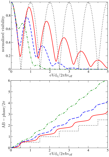
Figure 3: (Color online) Single-channel bias: dependence on arm length difference and interaction strength. Top: Normalized visibility as a function of bias voltage for $T_{a}=T_{b}=1/2.$ Black dotted line $d_{2}/d_{1}=1,$ $g/v_{f}=0.25$; red solid line $d_{2}/d_{1}=1.1$, $g/v_{f}=0.25$; blue dashed line $d_{2}/d_{1}=1.2$, $g/v_{f}=0.25$, green dot-dashed line $d_{2}/d_{1}=1.2$, $g/v_{f}=0.125$. Bottom: Phase of AB-fringes as a function of bias voltage for the same parameters.

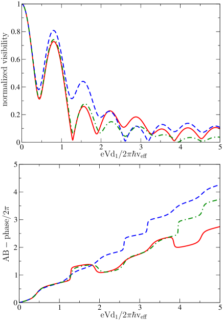
Figure 4: (Color online) Single-channel bias: dependence on $T_{a}$. Top: Normalized visibility as a function of bias voltage for $d_{2}/d_{1}=1.2$ and $g/v_{f}=0.25,$ $T_{b}=0.5$ and different $T_{a}.$ Red solid line $T_{a}=\sin^{2}\pi/8;$ blue dashed line $T_{a}=\sin^{2}3\pi/8;$ green dot-dashed line $T_{a}=\sin^{2}\pi/6.$ Bottom: Phase of AB-fringes as a function of bias voltage for the same parameters.

The dependence of interference on difference in arm lengths and on interaction strength is shown for an MZI with single-channel bias and $T_{a}=T_{b}=1/2$ in Fig. 3. For $d_{2}=d_{1}$ the visibility oscillates with constant amplitude as a function of bias voltage, following Eq. (52), and the phase of AB-fringes shows exact steps of height $\pi$ at the zeros of visibility. The energy scale of oscillations is $\varepsilon_{d}=\hbar v_{\mathrm{eff}}/d$ and diverges in the non-interacting limit. For $d_{1}\not=d_{2}$ the visibility develops a decaying envelope on the energy scale $\varepsilon_{+}$ or $\varepsilon_{-}$ (depending on the value of $\gamma$), minima in visibility are no longer exact zeros, and the steps in the phase as a function of bias are smooth.

Variations with the tunnelling probability $T_{a}$ are shown in Fig. 4. When the QPC $a$ is tuned away from the half-transparency, the visibility and the phase of AB-fringes become irregular functions of bias voltage. Changes in $T_{b}$ alter only the overall scale for the visibility, and not the form of its dependence on bias.

VI.2.2 Inteferometer with two-channel bias

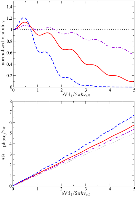
Figure 5: (Color online) Two-channel bias: dependence on arm length difference and interaction strength. Top: Normalized visibility as a function of bias voltage for $T_{a}=T_{b}=1/2$. Black dotted line $d_{2}/d_{1}=1,$ $g/v_{f}=0.25;$ dot-dashed violet line $d_{2}/d_{1}=1.05,$ $g/v_{f}=0.25;$ red solid line $d_{2}/d_{1}=1.1,$ $g/v_{f}=0.25$; blue dashed line $d_{2}/d_{1}=1.2$, $g/v_{f}=0.125$. Bottom: Phase of AB-fringes as a function of bias voltage for the same parameters.

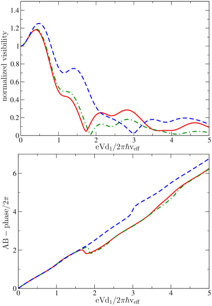
Figure 6: (Color online) Two-channel bias: dependence on $T_{a}$. Top: Normalized visibility as a function of bias voltage for $d_{2}/d_{1}=1.2$, $g/v_{f}=0.25,$ $T_{b}=1/2$ and different $T_{a}.$ Red solid line $T_{a}=\sin^{2}\pi/8;$ blue dashed line $T_{a}=\sin^{2}3\pi/8;$ green dot-dashed line $T_{a}=\sin^{2}\pi/6.$ Bottom: Phase of AB-fringes as a function of bias voltage for the same parameters.

The dependence of interference on difference in arm lengths and on interaction strength is shown for an MZI with two-channel bias and $T_{a}=T_{b}=1/2$ in Fig. 5. For equal arm lengths the visibility is independent of bias and the phase of AB-fringes varies linearly with voltage, following Eq. (55). For $d_{1}\not=d_{2}$ the visibility develops small amplitude oscillations and is suppressed at large bias: the voltage period of oscillations is consistent with the value $2\pi\hbar v_{\mathrm{eff}}/ed$ expected from Eq. (71). The variation of phase with voltage is no longer exactly linear but shows no well-defined steps.

Results for several values of $T_{a}$ are displayed in Fig. 6: oscillations of visibility with bias are irregular but some well-defined minima develop for values far from $T_{a}=1/2$.

VI.2.3 Suppression of visibility at high bias

From the discussion in Section VI.1 we expect the voltage scale for the suppression of visibility at high bias to be set by $\varepsilon_{\pm}$. Behaviour consistent with this is shown in Fig. 7: here $\gamma>1$ for all parameter sets, and $\varepsilon_{+}/e$ sets a common voltage scale to the envelope for visibility oscillations. We note that for $T_{a}=1/2$ this envelope is approximately Gaussian.

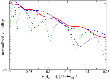
Figure 7: (Color online) Suppression of coherence at high bias: visibility on a logarithmic scale as a function of bias voltage. Two-channel bias: red solid line $d_{2}/d_{1}=1.1,$ blue dashed line $d_{2}/d_{1}=1.2$. Single-channel bias: green dotted line $d_{2}/d_{1}=1.1,$ violet dot-dashed line $d_{2}/d_{1}=1.2$. In all cases $g/v_{f}=0.25$ and $T_{a}=T_{b}=1/2.$

VII Discussion

In this section we discuss our results in relation to experimental observations and previous theoretical work. To summarise briefly: building on techniques developed in earlier studies Kovrizhin1 ; Kovrizhin2 we have presented exact analytical and numerical results for the non-equilibrium behaviour of an electronic Mach-Zehender interferometer built from quantum Hall edge states at filling factor $\nu=2$, using a model with only contact interactions. A key feature of the results is that, for an interferometer with nearly equal arm lengths, two scales are present in the dependence of fringe visibility on bias voltage: oscillations in visibility have the voltage period $2\pi v_{\mathrm{eff}}/ed$, with $d\approx d_{1}\approx d_{2}$, while their envelope falls off on the larger scale $2\pi v_{\mathrm{eff}}/e|d_{1}-d_{2}|$. A further feature is that oscillations in visibility are much clearer in one bias scheme (single-channel bias) than in an alternative scheme (two-channel bias). Finally, AB fringes show a varying degree of phase rigidity under small changes in bias: for single-channel bias it is perfect when arm lengths are equal, but decreases with increasing $|d_{1}-d_{2}|$; for two-channel bias it is absent if arm lengths are equal, and otherwise at most limited.

Some but not all aspects of these results match observations. Most importantly, the originally reported Heiblum2 ‘lobe pattern’ is reproduced by calculations for the experimentally appropriate single-channel bias scheme with $d_{1}\not=d_{2}$ (see Fig. 3). In addition, as previously discussed in the perturbative context, Sukhorukov the differences in behaviour between the two bias schemes (compare Ref. Heiblum2, with Ref. bieri08, ) are matched by differences in calculated behaviour (compare Fig. 3 with Fig. 5). On the other hand, as at most a few oscillations of visibility are observed in the lobe pattern, Heiblum2 ; bieri08 the voltage scales for oscillations and for their envelope are not well-separated: since the samples concerned are intended to have almost equal arm lengths, this is at variance with the behaviour of the model we study. Moreover, intentional changes in the length of an arm appear to have a much smaller effect experimentally Heiblum2 than in our calculations.

It is interesting to go beyond these qualitative comparisons and attempt an estimate of the key theoretical parameter, $v_{\mathrm{eff}}$, which characterises interaction strength in our model. This is possible using measurements by Roulleau and collaborators, described in Ref. RoulleauThese, . The relevant experiment, in the notation of our Fig. 1, involves applying separate biases to the channels $1\uparrow$ and $1\downarrow$, with the other two channels grounded. Specifically, applying a voltage to $1\uparrow$, this channel acts as a modulation gate, changing the phase of AB oscillations in conductance. From Fig. 5.17a of Ref. Roulleau, , a bias of 49$\mu$V generates a phase shift of $2\pi$ in a sample with $d_{1}=d_{2}=11.3\mu\mathrm{m}$. Using the results described in Section IV we obtain from these data the value $v_{\mathrm{eff}}=6.7\times 10^{4}\,\mathrm{ms}^{-1}$. Remarkably, this is very close to the estimate ($v_{\mathrm{eff}}=6.5\times 10^{4}\,\mathrm{ms}^{-1}$) obtained in Ref. Kovrizhin2, from a theoretical fit of an experiment on equilibration of QHE edge states, although in general $v_{\mathrm{eff}}$ is expected to vary with sample design and magnetic field strength.

Our results should also be compared with a body of earlier theoretical work, which (apart from the early study of Ref. Cheianov, ) can be separated into investigations of the effects of long range interactions, ChGV ; neder08 ; sim08 ; Kovrizhin1 ; Mirlin and calculations for the model Sukhorukov ; Mirlin with contact interactions that we have studied here. The initial treatment of this model Sukhorukov was perturbative in the tunnelling amplitude at the two QPCs, and so appropriate for $T_{a,b}\ll 1$ or $1-T_{a,b}\ll 1$, while an approximate non-perturbative approach has been described in Ref. Mirlin, . The advance we have presented here is to handle tunnelling exactly. The successes and weaknesses of the perturbative calculations Sukhorukov in accounting for observations are similar to the ones we have described above. In particular, the fact that the voltage scale for suppression of AB oscillations is set by the difference in arm lengths, and diverges for $d_{1}=d_{2}$ appears at the perturbative level. Knowing only the original, leading order result,Sukhorukov one might have hoped that contributions higher order in $T_{a}$ would eliminate AB oscillations at large bias for all $d_{1}-d_{2}$ (as happens when shot noise is introduced using a separate QPC levk ). The calculations we have described show (in agreement with the approximation of Ref. Mirlin, ) that this is not the case.

An implication of the work we have presented is that one must take account of long range interactions in order to understand in full experiments on non-equilibrium effects in MZIs. Calculations that do include long range interactions neder08 ; sim08 ; Kovrizhin1 successfully reproduce many aspects of the observations, but have been done for $\nu=1$ while much of the published data are for $\nu=2$. Approaches such as the one of Ref. Mirlin, that include both long range interactions and the two channels present at $\nu=2$ are therefore desirable. In this context, the results we have presented provide a testing ground for approximation schemes. Interestingly, the same model for QH edge states that we have studied here, of contact interactions at $\nu=2$, seems to account more successfully for experiments on relaxation of a non-equilibrium electron distribution pierre2010 ; Kovrizhin2 than for the behaviour of an MZI with equal length arms. While we have no detailed understanding of this difference, we point out that AB interference is a more sensitive probe of the QH edge than a measurement of the electron distribution. In particular, if as is likely, weak long range interactions are present in addition to contact interactions, they can be expected to suppress interference in a MZI at high bias ChGV without much changing quench2009 the observed relaxation process. In outlook, we hope that it will be possible to extend the techniques we have developed here to treat other phenomena in edge states far from equilibrium.

Appendix A Numerical evaluation of the tunnelling conductance

Here we outline the numerical procedure we use to obtain results for an interferometer with unequal arm lengths. The task is to evaluate Eq. (67), in which the average is taken with respect to the scattering state produced by QPC $a$. This scattering state is generated by the action of the operator $\hat{\mathcal{S}}_{a}$ on a Slater determinant describing filled Fermi seas that are defined by chemical potentials $A_{\pm}$. The scattering operators $\hat{\mathcal{S}}_{a}^{\dagger}\ldots\hat{\mathcal{S}}_{a}$ appearing in Eq. (67) can alternatively be taken to transform the operators they enclose rather than the state vectors, and the averages we require then have the general form

$$A_{ij}=\langle\hat{a}_{i}^{\dagger}e^{i\sum_{kl}H_{kl}\hat{a}_{k}^{\dagger}\hat{a}_{l}}\hat{a}_{j}\rangle,$$ (72)

where $\hat{a}_{i}^{\dagger}$ is an electron creation operator and the index $i$ labels both channel and energy eigenstate. Since $\sum_{kl}H_{kl}\hat{a}_{k}^{\dagger}\hat{a}_{l}$ is quadratic in fermion operators, we can use Wick’s theorem to obtain

$$A_{ij}=\det\hat{M}\times[\hat{n}\times\hat{M}^{-1}]_{ji},$$ (73)

with

$$\hat{M}\equiv\hat{I}+(e^{i\hat{H}}-\hat{I})\hat{n}\,.$$ (74)

Here $\hat{I}$ is an identity matrix and $\hat{n}$ is the density operator, which can be written in the basis of scattering states

$$n_{ij}\equiv\langle i|\hat{n}|j\rangle=\langle\hat{a}_{j}^{\dagger}\hat{a}_{i}\rangle.$$ (75)

The matrix $M$ has a similar form to those appearing in the problem of full counting statistics Klich and in nonequilibrium bosonization.gutman We evaluate Eq. (73) numerically using an energy eigenstate basis for a system of finite length $L$ with the eigenstates on a given channel occupied from the bottom of an energy window up to the corresponding chemical potential. We use at most about $2000$ states in each channel.

As a check we present in Fig. 8 a comparison of results from these numerical calculations at weak tunnelling with those from perturbation theory in tunnelling strength. The agreement is essentially perfect on the scale visible in our figures.

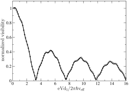
Figure 8: Comparison of the exact result (circles) with perturbation theory (solid line) in the small tunnelling limit for $g/v_{f}=0.75$ and $d_{2}/d_{1}=1.2.$

Appendix B Perturbation theory in the small tunnelling limit

In this appendix we recall the results of perturbation theory in tunnelling strength and compare behaviour for $T_{a,b}=1/2$ with that at weak tunnelling.

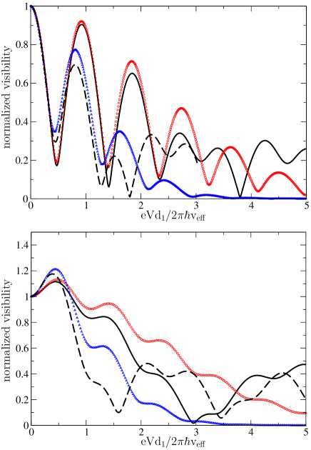
Figure 9: (Color online) Comparison of the exact results at $T_{a}=T_{b}=1/2$ (symbols) with those at weak tunnelling (lines). Top: single-channel bias; bottom: two-channel bias. Solid black line and red circles: $d_{2}/d_{1}=1.1$; dashed black line and blue triangles: $d_{2}/d_{1}=1.2$. All data for $g/v_{f}=0.25$.

Perturbation theory in tunnelling strength was applied to MZIs at $\nu=1$ in Refs. Cheianov, and ChGV, , and at $\nu=2$ in Ref. Sukhorukov, . For the model we study, the current through the interferometer at small $v_{a},v_{b}$ is given by

$$I(V)=-\frac{2e}{\hbar^{2}}\int_{-\infty}^{\infty}dt\ [(v_{a}^{2}+v_{b}^{2})e^{-ieVt/\hbar}i\mathrm{Im}[g(0,t)^{2}]\\ +\{v_{a}v_{b}e^{i\varphi_{AB}}e^{-ieV(t-t_{0})/\hbar}i\mathrm{Im}[g(d_{1},t)g(d_{2},t)]\\ +\mathrm{c.c}.\}],$$ (76)

where $g(x,t)$ is

$$g(x,t)=\frac{i}{2\pi}\frac{1}{(x-v_{+}t+ia)^{1/2}}\frac{1}{(x-v_{-}t+ia)^{1/2}}.$$

Here $t_{0}=d_{1}v/v_{+}v_{-}$ for single-channel bias, and $t_{0}=d_{1}/v_{+}$ for two-channel bias. The integral in the Eq. (76) can be evaluated Sukhorukov analytically in the strong coupling limit $v_{+}/v_{-}\gg 1$, giving (for example) with two-channel bias the visibility

$$\mathcal{V}_{\mathrm{pert}}^{(TCB)}(V)=\mathcal{V}_{0}|J_{0}(eV[d_{2}-d_{1}]/2\hbar v_{-})|,$$ (77)

where $J_{0}(x)$ is a Bessel function. For general interaction strength and arm lengths one can evaluate Eq. (76) numerically. We compare the results of these calculations with our results at $T_{a}=T_{b}=1/2$ in Fig. 9, using the same parameters as in Figs. 3 and 5. We note that while the qualitative behaviour is similar for both strong and weak tunnelling, specific features differ greatly, especially at large bias. These differences appear to be much greater than those found in the approximate treatment of finite tunnelling strength Mirlin (compare our Fig. 3 with Fig. 5 of Ref. Mirlin, ).

References

- (1) Y. Ji, Y. C. Chung, D. Sprinzak, M. Heiblum, D. Mahalu, and H. Shtrikman, Nature 422, 415 (2003).
- (2) I. Neder, M. Heiblum, Y. Levinson, D. Mahalu, and Y. Umansky, Phys. Rev. Lett. 96, 016804 (2006).
- (3) L. V. Litvin, H.-P. Tranitz, W. Wegscheider, and C. Strunk, Phys. Rev. B 75, 033315 (2007).
- (4) P. Roulleau, F. Portier, D. C. Glatti, P. Roche, A. Cavanna, G. Faini, U. Gennser, and D. Mailly, Phys. Rev. B 76, 161309(R) (2007).
- (5) I. Neder, F. Marquardt, M. Heiblum, D. Mahalu, and V. Umansky, Nature Physics 3, 534 (2007).
- (6) I. Neder, M. Heiblum, D. Mahalu, and V. Umansky, Phys. Rev. Lett. 98, 036803 (2007).
- (7) L. V. Litvin, A. Helzel, H.-P. Tranitz, W. Wegscheider, and C. Strunk, Phys. Rev. B 78, 075303 (2008).
- (8) P. Roulleau, F. Portier, P. Roche, A. Cavanna, G. Faini, U. Gennser, and D. Mailly, Phys. Rev. Lett. 100, 126802 (2008).
- (9) P. Roulleau, Ph.D. thesis, Universite Pierre et Marie Currie - Paris 6, (2008), http://tel.archives-ouvertes.fr/docs/00/44/37/03/PDF/These.pdf.
- (10) P. Roulleau, F. Portier, P. Roche, A. Cavanna, G. Faini, U. Gennser, and D. Mailly, Phys. Rev. Lett. 101, 186803 (2008).
- (11) P. Roulleau, F. Portier, P. Roche, A. Cavanna, G. Faini, U. Gennser, and D. Mailly, Phys. Rev. Lett. 102, 236802 (2009).
- (12) E. Bieri, M. Weiss, O. Götkas, M. Hauser, C. Schönenberger, and S. Oberholzer, Phys. Rev. B 79, 245324 (2009).
- (13) L. V. Litvin, A. Helzel, H.-P. Tranitz, W. Wegscheider, and C. Strunk, Phys. Rev. B 81, 205425 (2010).
- (14) G. Seelig and M. Büttiker, Phys. Rev. B 64, 245313 (2001); F. Marquardt and C. Bruder, Phys. Rev. Lett. 92, 056805 (2004); H. Förster, S. Pilgram, and M. Büttiker, Phys. Rev. B 72, 075301 (2005); F. Marquardt, Europhys. Lett. 72, 788 (2005).
- (15) E. V. Sukhorukov and V. V. Cheianov, Phys. Rev. Lett. 99, 156801 (2007).
- (16) J. T. Chalker, Y. Gefen, M. Y. Veillette, Phys. Rev. B 76, 085320 (2007).
- (17) I. P. Levkivskyi and E. V. Sukhorukov, Phys. Rev. B 78, 045322 (2008).
- (18) I. P. Levkivskyi and E. V. Sukhorukov, Phys. Rev. Lett. 103, 036801 (2009).
- (19) I. Neder and E. Ginossar, Phys. Rev. Lett. 100, 196806 (2008).
- (20) S.-C. Youn, H.-W. Lee, and H.-S. Sim, Phys. Rev. Lett. 100, 196807 (2008).
- (21) D. L. Kovrizhin and J. T. Chalker, Phys. Rev. B 80, 161306 (2009); 81, 155318 (2010).
- (22) M. Schneider, D. Bagrets and A. Mirlin, Phys. Rev. B 84, 075401 (2011).
- (23) B. I. Halperin, Phys. Rev. B 25, 2185 (1982).
- (24) X. G. Wen, Phys. Rev. Lett. 64, 2206 (1990); Phys. Rev. B 43, 11025 (1991).
- (25) Jan von Delft and H. Schoeller, Ann. Phys. (Leipzig) 7, 225 (1998).
- (26) T. Giamarchi, Quantum Physics in One Dimension, (Oxford University Press, Oxford, 2004).
- (27) M. Fabrizio and A. Parola, Phys. Rev. Lett. 70, 226 (1993).
- (28) Jan von Delft, G. Zarand and M. Fabrizio, Phys Rev. Lett, 81, 196 (1998); G. Zarand and Jan von Delft, Phys. Rev. B, 61, 6918 (2000); arXiv:cond-mat/9812182.
- (29) D. L. Kovrizhin and J. T. Chalker, Phys. Rev. Lett. 109, 106403 (2012).
- (30) H. le Sueur, C. Altimiras, U. Gennser, A. Cavanna, D. Mailly, F. Pierre, Phys. Rev. Lett. 105, 056803 (2010).
- (31) D. L. Kovrizhin and J. T. Chalker, Phys. Rev. B 84, 085105 (2011).
- (32) L. S. Levitov and G. B. Lesovik, JETP Lett. 58, 230 (1993); L. S. Levitov in Quantum Noise in Mesoscopic Systems, ed. Yu. V. Nazarov (Kluwer, Amsterdam, 2003); I. Klich ibid.
- (33) D. B. Gutman, Y. Gefen, and A. D. Mirlin, Phys. Rev. Lett. 101, 126802 (2008); Phys. Rev. B 81, 085436 (2010).