Cluster-size heterogeneity in the two-dimensional Ising model

Abstract

We numerically investigate the heterogeneity in cluster sizes in the two-dimensional Ising model and verify its scaling form recently proposed in the context of percolation problems [Phys. Rev. E 84, 010101(R) (2011)]. The scaling exponents obtained via the finite-size scaling analysis are shown to be consistent with theoretical values of the fractal dimension $d_{f}$ and the Fisher exponent $\tau$ for the cluster distribution. We also point out that strong finite-size effects exist due to the geometric nature of the cluster-size heterogeneity.

In studies of critical phenomena, the finite-size scaling (FSS) has proved to be an extremely fruitful approach, owing to the recent development in computation Newman and Barkema (1999). It is through a crossover effect that this method connects numerical results to theoretical understanding so successfully. Although a typical simulation of a lattice system can only deal with a finite length scale $L$, one may regard $L$ as a relevant scaling variable in the following way Cardy (1996): Under a scaling transformation by zooming factor $b$, i.e., $L^{-1}\rightarrow bL^{-1}\rightarrow b^{2}L^{-1}\cdots\rightarrow b^{n}L^{-1}$, the scale invariance of critical phenomena suggests that the singular part of the free energy $f$ will transform as

$$f(u_{t},L^{-1})=b^{-d}f(b^{y_{t}}u_{t},bL^{-1})=b^{-nd}f(b^{ny_{t}}u_{t},b^{n}L^{-1}),$$ (1)

where $u_{t}$ is a thermal scaling variable and $y_{t}=1/\nu$ is its eigenvalue. The quantity $\nu$ is called the correlation-length exponent since the correlation length $\xi$ behaves as $\xi\sim|t|^{-\nu}$ with $t\equiv(T-T_{c})/T_{c}$, where $T_{c}$ denotes the critical temperature. The scaling variable $u_{t}$ is proportional to $t/t_{0}$ near a fixed point of this renormalization-group (RG) transformation, where $t_{0}$ is a nonuniversal scale specific to the system. This linear approximation remains valid until the system reaches a point where $b^{ny_{t}}|t/t_{0}|\sim\mathcal{O}(1)$. Comparing this with Eq. (1), we find that $f$ is only weakly dependent on the first argument in this region and thus can be written as

$$f(u_{t},L^{-1})\sim\left|t/t_{0}\right|^{d\nu}f\left(|t/t_{0}|^{-\nu}L^{-1}\right).$$ (2)

In other words, the crossover occurs when $|t|\sim L^{-1/\nu}$, and therefore, $L$ usually enters an FSS form accompanied by the exponent $-1/\nu$. Recalling that $\xi\sim|t|^{-\nu}$, we see that the argument on the right-hand side of Eq. (2) means $\xi/L$, expressing the competition between $\xi$ and $L$.

The cluster-size heterogeneity $H$ suggested by Lee et al. has been devised in the context of recent debates on explosive percolation and defined as the number of distinct cluster sizes Lee et al. (2011). For brevity, we will call it simply “the heterogeneity” henceforth, but it is to be noted that only sizes (or volumes) of clusters matter in calculation of $H$, irrespective of shapes of clusters. Noh et al. have shown that this quantity can be applied to ordinary percolation as well Noh et al. (2011): They have calculated $H=H(p)$ with finite $L$’s, where $p$ means occupation probability, and found that $H(p)$ has a peak at $p=p^{\ast}$, which approaches the true percolation threshold $p_{c}$ as $L$ increases. It is a typical signature to detect the percolation transition. One may well expect that the deviation of $p^{\ast}$ from the true $p_{c}$, related to the thermal scaling variable in percolation, will be described as $\sim L^{-1/\nu}$ for the same reason as explained above. However, Noh et al. Noh et al. (2011) have revealed that the FSS form for $H$ is obtained with another exponent $\nu_{H}$ than $\nu$. This exponent $\nu_{H}$ can be argued in the following way: Let us consider the probability distribution of cluster sizes $s$, which scales as

$$P(s)\sim s^{-\tau}e^{-s/s_{c}},$$

with the characteristic cluster size $s_{c}\sim|t|^{-1/\sigma}$. Here $t=p-p_{c}$ in percolation problem and the scaling exponent $\tau$ is called the Fisher exponent. If the system is off-critical, its cluster sizes will be simply found between $1$ and $s_{c}$ so that $H\sim s_{c}\sim|t|^{-1/\sigma}$. On the other hand, if $|t|\ll 1$, $H$ is limited by the finite size $L$ and its scaling relation becomes different: We first consider $s_{n}$ such that $P(s_{n})\sim s_{n}^{-\tau}\sim 1/N_{c}$, where $N_{c}$ is the total number of clusters. In fact, since the typical cluster size is $\sum sP(s)\sim\mathcal{O}(1)$, $N_{c}$ is comparable to the total number of points $N$. For a $d$-dimensional system, it is obvious that $L$ is related to $N$ by $N\sim L^{d}$. Furthermore, since $P(s_{n})\sim 1/N_{c}$, there are few clusters above $s_{n}$ and their contribution to $H$ will be much smaller than those with $s<s_{n}$. It is likely to find at least one cluster for each $s<s_{n}$ since $P(s<s_{n})>1/N_{c}$, and thus it is plausible that $H\sim s_{n}\sim N^{1/\tau}$. To sum up, $H$ is expected to have the following behavior

$$H(t,L)\rightarrow\left\{\begin{array}[]{ll}L^{d/\tau}&\mbox{if~{}~{}}|t|\ll 1\\ |t|^{-1/\sigma}&\mbox{otherwise.}\end{array}\right.$$

Note that it is not $\xi$ and $L$ that actually compete here. The competition is rather between $s_{c}$ and $s_{n}$, reflecting the limitation in observing large clusters due to the finite system size. The appropriate FSS form for describing $H$ should be, therefore,

$$H(t,L)=L^{d/\tau}F_{H}\left(|t|L^{1/\nu_{H}}\right)$$ (3)

with $\nu_{H}\equiv\tau/(d\sigma)$. This FSS form is readily supported by numerical results in percolation Noh et al. (2011).

The ferromagnetic Ising model is one of the simplest and the most important models in statistical mechanics. When the dimensionality $d$ is higher than unity, it undergoes an order-disorder transition at a critical temperature $T_{c}$. Near the critical temperature $T_{c}$, the magnetic order parameter $m$ scales as a power-law form $m\sim\left|t\right|^{\beta}$ and the corresponding FSS form is given as $m=L^{-\beta/\nu}F_{m}(|t|L^{1/\nu})$ Goldenfeld (1993); Newman and Barkema (1999). Instead of this conventional order parameter, we will look into the system in terms of cluster statistics such as heterogeneity in the present study, where a cluster in the Ising model is defined as a set of nearest-neighboring spins with the same direction. We first recall that Suzuki Suzuki (1983) has conjectured that the fractal dimension of an Ising cluster is $d_{f}=d-\beta/\nu$. For instance, for $d=2$, this conjecture suggests $d_{f}=15/8$ by inserting $\beta=1/8$ and $\nu=1$ into the relation. However, this suggested fractal dimension is not consistent with numerical results Cambier and Nauenberg (1983). The reason is that there are actually two contributions in forming a cluster: One is due to the correlation due to the spin interaction, while the other is a purely geometric contribution which survives even in the infinite-$T$ limit Coniglio and Klein (1980). For example, one has a chance to find a giant cluster in the Ising model in the triangular lattice at $T\rightarrow\infty$ since each site has a spin state of either up or down randomly with probability $1/2$, which coincides with the site-percolation threshold in the triangular lattice Coniglio et al. (1977). In order to separate the geometric effect from the correlation effect, one may consider bond-occupation probability $p_{B}$ inside a cluster Coniglio and Klein (1980); Coniglio and Peruggi (1982); Vanderzande (1992). These bonds are only to define connectivity between neighboring spins in the same direction and do not affect the spin interaction. Therefore, we are back to the original cluster statistics with $p_{B}=1$, which is of our primary concern. When $p_{B}=0$, on the other hand, the system reduces to the pure Ising model, with two relevant eigenvalues associated with $t$ and $h$, respectively, where $h$ is an external magnetic field. It means that we need think of the RG parameter space as $(t,h,p_{B})$. Since $p_{B}$ is related to the random bond percolation, the $p_{B}$-axis will have one unstable fixed point, separating two stable fixed points. A careful RG analysis shows that the stable fixed point at higher $p_{B}$ is actually a tricritical point Stella and Vanderzande (1989); Vanderzande (1992). Suzuki’s argument that $d_{f}=15/8$ is indeed true at the unstable fixed point describing Fortuin-Kasteleyn clusters Fortuin and Kasteleyn (1972), but one should note that the critical behavior is not given by this point, because it is the tricritical point that attracts the RG flow starting from $p_{B}=1$. Conformal invariance then predicts that the fractal dimension for geometrical clusters of the two-dimensional (2D) Ising model is $d_{f}=187/96$ from tricritical exponents Stella and Vanderzande (1989). This prediction is well substantiated by numerical results in Refs. Fortunato (2002); Janke and Schakel (2005); Winter et al. (2008).

Now we consider the cluster-size distribution in the square lattice at the critical temperature $T_{c}=2/\ln(1+\sqrt{2})\approx 2.27$ in units of $J/k_{B}$, where $k_{B}$ is the Boltzmann constant. This distribution follows a power law with exponent $\tau$ in the thermodynamic limit, and the exponent $\tau$ follows the relation Christensen and Moloney (2005),

$$\tau=1+d/d_{f},$$ (4)

which is derived from cluster statistics as in percolation. In other words, one can check the predictions of $d_{f}$ by measuring $\tau$ from the cluster-size distribution.

We perform Monte Carlo (MC) simulations of the Ising model using the Metropolis and the Wolff algorithms Newman and Barkema (1999) in 2D $L\times L$ square with under the periodic-boundary condition. For most simulations we use $L=20,40,60,80,100$ and $160$, but $L=320$ is also used when required. We mostly use the Wolff algorithm for efficiency, and the Metropolis algorithm only for a consistency check. We start from a temperature much higher than $T_{c}$, and then slowly decrease $T$, measuring equilibrium quantities at each temperature. All results are obtained from averages over $5\times 10^{5}$ MC steps, after disregarding the first $5\times 10^{5}$ MC steps for equilibration. We first choose a snapshot of a spin configuration in equilibrium and identify all the clusters in the system. Then we count how many different sizes of the clusters are found in spin-up and down directions, respectively. The cluster heterogeneity is then calculated as the sum of these two numbers, one in the spin-up direction, the other in the spin-down direction. Our brute-force approach in counting all the cluster sizes works as a main bottleneck in increasing the system size: For example, the CPU time spent for $L=160$ roughly amounts to $4\times 10^{2}$ hours. Although limited by such a practical difficulty, our results nevertheless nicely agree with the prediction in the conformal field theory (see Table 1).

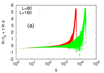
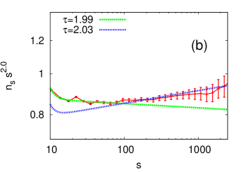
Figure 1: (Color online) (a) Cluster size distributions $n_{s}$ for the Ising model in the $L\times L$ square lattices at the critical temperature $T_{c}$. This figure is plotted in the form of $\ln(n_{s}s^{\tau})$ versus the cluster size $s$ with the predicted exponent $\tau=1+d/d_{f}=379/187\approx 2.03$. The errorbars are of about the same sizes as the symbols for the scaling regime of $s\lesssim 1000$ and omitted for better visibility. (b) Estimation of the Fisher exponent $\tau$ for $L=320$ (see text for details). Log-binned $n_{s}$ are shown in the form of $n_{s}s^{2.0}$ versus $s$ (symbols) and the lines are results from the curve-fitting to $n_{s}s^{\tau}\sim 1+As^{-\Delta}$ with $\tau$ fixed to $2.03$ and $1.99$. It is clearly seen that the correct value of $\tau$ is between 1.99 and and 2.03 and we thus conclude $\tau=2.01(2)$.

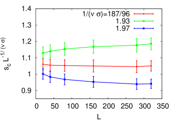
Figure 2: (Color online) Characteristic cluster size $s_{c}$ in the $L\times L$ square lattices at $T_{c}\approx 2.27(J/k_{B})$. The data points are scaled by $L^{-1/({\nu\sigma})}$ with varying $1/{(\nu\sigma)}$ around $187/96\approx 1.95$, so that all the data points lie on a horizontal line within error bars. This estimate results in $1/(\nu\sigma)=1.95(2)$.

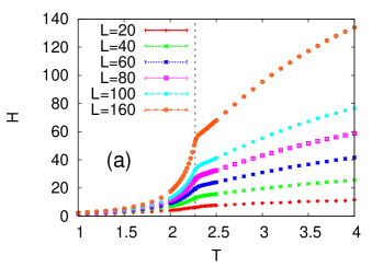
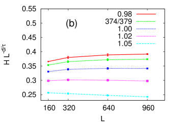
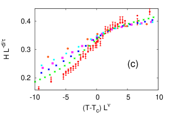
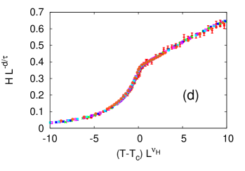
Figure 3: (Color online) (a) Heterogeneity $H$ is drawn as a function of $T$ for the 2D Ising model in the $L\times L$ square lattices. The dotted line indicates $T_{c}$, and error bars are smaller than the data points. (b) We obtain $X_{H}=1.00(2)$ by scaling $H(t=0,L)$ as a function of $L$ for the largest sizes at $T_{c}$. (c) Scaling by using the conventional FSS ansatz in Eq. (7) with $\nu=1$ and $X_{H}=374/379\approx 0.99$. (d) Scaling collapse using Eq. (8) with $\nu_{H}=379/192\approx 1.97$ and $X_{H}=374/379\approx 0.99$.

The cluster distribution in the 2D Ising model obeys the following form Christensen and Moloney (2005) :

$$n_{s}=s^{-\tau}F_{n_{s}}\left(|t|s^{x}\right),$$ (5)

where $n_{s}$ is number of clusters with size $s$. This scaling form is valid near $T_{c}$ and with zero magnetic field. At $T=T_{c}$, it leads to $n_{s}\sim s^{-\tau}$. The scaling relation Eq. (4) with $d_{f}=187/96$ for the 2D Ising model gives us $\tau=379/187\approx 2.03$, which is shown to be consistent with our numerical results as shown in Fig. 1(a). For a more careful analysis, we allow the correction to the scaling form as $n_{s}\sim s^{-\tau}(1+As^{-\Delta}+\ldots)$ with a constant $A$ and a correction exponent $\Delta>0$ and apply it for $L=160$ and $320$. We find that our numerical results are described sufficiently well by $\tau=2.01(2)$ as shown in Fig. 1(b). However, more precise estimation of $\tau$ is a formidable task, since it depends on the choice of the scaling region of $s$ and also a further increase of $L$ can alter the estimation made for smaller sizes. A better way is then to cross check with the outcomes of scaling relations as to be discussed below.

The peaks at the tail part in Fig. 1(a) are due to giant clusters, exclusion of which yields the monotonically decreasing distribution without the peaks instead. This allows us to approximate $F_{n_{s}}\left(|t|s^{x}\right)$ as an exponentially decaying function $e^{-s/s_{c}}$ where $s_{c}$ is the characteristic cluster size similar to the one used in percolation Noh et al. (2011). We may also identify $s_{c}$ with a peak position of $n_{s}$ near the tail in Fig. 1(a), and either way gives similar scaling behavior, $s_{c}\sim|t|^{-1/\sigma}$. In order to obtain the exponent $\sigma$, we apply the standard technique of the FSS method to $s_{c}$:

$$s_{c}=L^{\frac{1}{\nu\sigma}}F_{s_{c}}\left(|t|L^{1/\nu}\right).$$ (6)

The exponent $\sigma$ can be then obtained by analyzing simulation results with varying $L$ at $T=T_{c}$, by which we estimate the value of the exponent $1/{(\nu\sigma)}\approx 1.95(2)$ (see Fig. 2). Using the correlation-length exponent $\nu=1$ of the 2D Ising model, $1/\sigma\approx 1.95(2)$ is numerically obtained. The scaling relation $\sigma=1/(\nu d_{f})$ allows us to check our numerical results with the predicted value $1/\sigma=187/96\approx 1.95$ as shown in Fig. 2. Again the agreement is compelling, and our estimate favors this value over Suzuki’s conjecture $15/8=1.875$.

We next carry out the FSS analysis of $H$ in Fig. 3. First, we scale our numerical results [see Fig. 3(a)] using a conventional FSS form:

$$H(t,L)=L^{X_{H}}F_{H}\left(tL^{1/\nu}\right),$$ (7)

with a scaling exponent $X_{H}$. Although we can find the scaling exponent $X_{H}\approx 1.00(2)$ by numerically observing $H(t=0,L)$ as a function of $L$ [see Fig. 3(b)], we cannot observe scaling collapse with $\nu=1$ as shown in Fig. 3(c). Consequently, the argument of $F_{H}$ in the conventional FSS form Eq. (7) cannot be valid for $H$. This implies also that the correct scaling form should take into account the competition between cluster sizes as in percolation. By the same reasoning as above, a new scaling form is expected to be

$$H(t,L)=L^{d/\tau}F_{H}(tL^{1/\nu_{H}}),$$ (8)

where $\nu_{H}=\tau/(d\sigma)$. Using $\tau=379/187$ and $1/\sigma=d_{f}=187/96$, we expect the exponent to be $\nu_{H}=379/192\approx 1.97$, which indeed leads to a scaling collapse in a good quality [see Fig. 3(d)]. In addition, our numerical estimate $d/\tau=1.00(2)$ contains the theoretical prediction $374/379\approx 0.99$ within the error bar. We have obtained basically the same scaling behavior for heterogeneity in the triangular lattice as well (not shown), confirming its universality in the 2D Ising model. Our results are summarized in Table 1.

Figure 4: Heterogeneity in the square lattices as a function of $L$, when each site is assigned a random spin state between up and down at $T\rightarrow\infty$. Note that the horizontal axis is drawn on a logarithmic scale. Error bars are shown but smaller than the data points.

An interesting point in Fig. 3(a) is that $H$ keeps increasing as $L$ grows even though $T$ is far higher than $T_{c}$. Recall that all the correlation due to spin interaction is destroyed in the infinite-$T$ limit, where we are back to the percolation case. For the square lattice, the site-percolation threshold is $p_{c}^{\rm square}=0.59274602(4)$ Ziff (2011), while the infinite-$T$ Ising model corresponds to $p=1/2$ due to the up-down symmetry. Since Noh et al. have argued that $H\sim\ln L$ when $|p-p_{c}|\gg L^{-1/\nu_{H}}$ Noh et al. (2011), we expect that $H$ should have the logarithmic divergence for the infinite-$T$ Ising model, which is confirmed by our numerical results (Fig. 4). It is slower than the power-law divergence of $L^{d/\tau}$ at $T_{c}$, so there will develop a peak at $T=T_{c}$ at a large $L$. The existence of such a peak should be true for the Ising model in the triangular lattice, too: As mentioned above, one can find a percolating phase in the infinite-$T$ limit since $p_{c}^{\rm triangle}=1/2$. The divergence at infinite $T$ will be therefore described by 2D percolation exponents such as $H\sim L^{182/187}$, which is slightly slower than the Ising case of $H\sim L^{374/379}$ at $T=T^{\rm triangle}_{c}=4/\ln 3\approx 3.64$ Wannier (1945). Returning back to the square lattice, since we have a good reason to believe the existence of a peak at $T=T_{c}$ for a large $L$, the monotonic shape of the scaling function in Fig. 3(b) suggests that our observation might be still subject to corrections to scaling. We have indeed numerically found that the the logarithmic function $H(L)$ is hardly distinguishable from linear increase when $L<\mathcal{O}(10^{3})$, which explains the increase of $H(L)$ in Fig. 3(a).

Table 1: Scaling exponents for heterogeneity of the 2D Ising model. The numerical values are obtained by Monte Carlo calculations in this work, whereas the analytic values are from tricritical exponents in the conformal field theory.

	$d_{f}$	$\tau$	$d/\tau$	$\nu_{H}$
numerical	1.95(2)	2.01(2)	1.00(2)	1.96(5)
analytic	$187/96$	$379/187$	$374/379$	$379/192$
	$\approx 1.95$	$\approx 2.03$	$\approx 0.99$	$\approx 1.97$

In summary, we have shown that the cluster-size heterogeneity $H$ of the 2D Ising model is scaled by the recently suggested FSS form using the exponent $\nu_{H}$ Noh et al. (2011), instead of the correlation-length exponent $\nu$. The finite-size effects in measuring this quantity are quite substantial, especially if compared to those in percolation. We have argued the main reason that $H$ does not converge to a constant as the system size increases when $T>T_{c}$ but still has weak divergence due to its geometric nature. In spite of this difficulty, the scaling exponents at $T=T_{c}$ are in nice agreement with theoretical predictions (see Table 1). This justifies the validity of this observable as well as the use of $\nu_{H}$ instead of $\nu$ in the FSS analysis of the Ising system.