The network source location problem: ground state energy, entropy and effects of freezing

Abstract

Ground state entropy of the network source location problem is evaluated at both the replica symmetric level and one-step replica symmetry breaking level using the entropic cavity method. The regime that is a focus of this study, is closely related to the vertex cover problem with randomly quenched covered nodes. The resulting entropic message passing inspired decimation and reinforcement algorithms are used to identify the optimal location of sources in single instances of transportation networks. The conventional belief propagation without taking the entropic effect into account is also compared. We find that in the glassy phase the entropic message passing inspired decimation yields a lower ground state energy compared to the belief propagation without taking the entropic effect. Using the extremal optimization algorithm, we study the ground state energy and the fraction of frozen hubs, and extend the algorithm to collect statistics of the entropy. The theoretical results are compared with the extremal optimization results.

I Introduction

Statistical physics methods and ideas inherited from studies of disordered systems play an important role in providing theoretical insights and developing low complexity algorithms for combinatorial optimization problems or constraint satisfaction problems Mézard and Parisi (2001, 2003); Mézard and Montanari (2009). These problems become subjects of interest across a variety of different disciplines such as computer science, discrete mathematics, statistical physics, engineering and computational biology Mézard and Montanari (2009). One archetype that involves both continuous and discrete variables is the network source location problem where we try to find optimal location of sources in a transportation network with an optimal flow pattern. Studies on this source location problem Wong and Saad (2006); Yeung and Wong (2009a, b, 2010) are practically relevant to network design and optimization Yeung and Saad (2012) and can have widespread applications in the field of operations research Rardin (1998).

In the source location problem, transportation networks are assumed to be composed of nodes with either a surplus or a deficiency of resources. How to distribute the resources and to replace some deficient nodes by resource providing ones becomes an important problem in network optimization. After the optimization, the remaining deficient nodes serve as consumer nodes and a network-wide satisfaction is achieved. A series of discontinuous transitions with different configurations of the source and consumer nodes Yeung and Wong (2009a, 2010) can be observed by varying model parameters. Two of them are the singlet regime where the consumer nodes are isolated and the doublet regime where the consumer nodes can be paired or isolated. Even in the singlet regime, there exist a glassy phase in which optimizing the location of sources becomes algorithmically hard, which is most likely due to the emergence of long range frustrations Zhou (2005a, b).

In this work, we apply the entropic cavity method to evaluate the typical value of the ground state entropy in the singlet regime and probe the entropic effects. The entropic cavity method has been used to compute the ground state entropy of the minimal vertex cover (MVC) problem Zhou and Zhou (2009) and to study entropic effects in the channel coding problem and budget-constrained auctions Huang and Zhou (2009); Altarelli et al. (2009). The purpose of this paper is to consider the benefits brought by including the entropic effects properly, especially in terms of solutions (optimal assignments of source locations) found by improved message passing algorithms. Hereafter, we identify an assignment to be optimal if it yields the minimal energy cost in a specific regime (e.g., the singlet or doublet connection pattern). For verification, a standard implementation of the extremal optimization Boettcher and Percus (2001) is used to study the energetic properties, and this is adapted as a biased sampling method for the ground states which appears for small systems sufficient to enumerate all the ground states and frozen variables.

The rest of this paper is organized as follows. The source location problem is defined in detail in Sec. II. Following this definition we provide more details on the related literatures and previous results. The analysis at both the replica symmetric (RS) level and one-step replica symmetry broken ($1$RSB) level by the entropic cavity method is presented in Sec. III. The extremal optimization (EO) is developed; numerical and theoretical results are compared. In Sec. IV, experimental studies of the proposed maximal decimation and reinforcement strategy are carried out. Conclusion and some future directions are given in Sec. V. Some technical details are given in the Appendices.

II The source location problem

The facility location problem is an important problem in management science, since the placement of facilities at optimal positions in a network is able to provide efficient services while minimizing the logistics cost Revelle et al. (1977). The services may be public ones that concern the well-being of all citizens, such as ambulance service or public schools, or they may be private ones that concern the sphere of influence and maintenance cost of retailing companies Revelle (1986). Similar issues exist in wireless sensor networks Al-Karaki and Kamal (2004); Frey et al. (2009), in which sensors are deployed in an arena for purposes such as surveillance, fire detection, and collection of meteorological and pollution data. Due to the limited battery size of the sensors, minimizing the transportation cost becomes an essential issue to prolong the life span of the networks. However, the traditional approach to the problem is integer programming, whose complexity scales up rapidly with system size, and solutions for large-scale systems depend on heuristics Pirkul and Jayaraman (1998).

In this paper, we consider a transportation network of $N$ nodes in which resources are transported through the links, so that the resource demands of all nodes are satisfied. There are two kinds of nodes. The surplus nodes supply the resources and the deficient nodes have demands for resources. To the deficient nodes $i$ is associated a capacity $\Lambda_{i}=-1$, corresponding to the amount of resources consumed by $i$, and to the surplus nodes $i$ is associated a sufficiently large capacity $\Lambda_{i}=A\gg 1$, corresponding to the amount of resources it can provide. This scenario is typical in many modern applications of network traffic optimization, such as logistic networks and sensor networks, where the surplus nodes represent distribution centers in logistic networks or base stations in sensor networks.

The version of the source location problem considered in this paper is an optimization problem in the space of real-valued variables $x_{ij}$ and the Boolean variables $s_{i}$. The variables $s_{i}$ defined over the set of deficient nodes $\mathcal{D}$ are indicator functions ($1=$ true, $0$ false) for an installation, which is a reassignment of a deficient node capacity from $-1$ to $+A$ (making it behave as a surplus node). For each link we also define a real-valued flow $x_{ij}$ ( $=-x_{ji}$) from node $j$ to $i$. Those deficient nodes not reassigned ($s_{i}=0$) will be called consumer nodes and will have a net inward flow; all other nodes are called source nodes and will have zero, or positive net outward flow. In a valid assignment either a deficient node $i$ must be installed as a source node ($s_{i}=1$), or the flows are required to satisfy the non-negativity constraints of the final resource, defined by $\xi_{i}$ for every node, i.e.,

$$\xi_{i}\equiv\Lambda_{i}+\sum_{j\in\partial i}x_{ij}\geq 0,$$ (1)

where $\partial i$ denotes neighbors of node $i$. To valid flows and installations is further associated the energy

$$E=\sum_{\left(ij\right)}\frac{x_{ij}^{2}}{2}+\frac{u^{2}}{2}\sum_{i\in\mathcal{D}}s_{i}.$$ (2)

The task will be to optimize over valid flows and installations to minimize this quantity. The first term is the total transportation cost summed over each link $(ij)$. The transportation cost on link $(ij)$ is quadratic in the flow. The quadratic function is chosen because of its convex property, which tends to balance the traffic load among the links; other convex functions can work equally well Banavar et al. (2000); Shao and Zhou (2007); Bohn and Magnasco (2007). The second term is the installation cost of converting a deficient node to a source node.

We will be interested in studying an ensemble of diluted networks in which each node has the same degree $C$. The locations of the surplus and deficient nodes are random, with a fraction of surplus nodes given by $\phi_{s}$, hence capacities are assigned uniformly at random according to the distribution $\rho(\Lambda)=\phi_{s}\delta(\Lambda-A)+(1-\phi_{s})\delta(\Lambda+1)$. Other ensembles are certainly interesting, and our analysis can be easily extended to networks with fluctuating degrees (e.g., Erdös-Rényi random networks), or with other distributions of $\Lambda$. Many interesting phenomena can be exactly analyzed in this restricted setting, with implications for technologically relevant large networks.

II.1 Known results and developments with respect to related models

It has been previously shown that the optimal set of suppliers (source locations) can be obtained by assuming that all deficient nodes are consumer nodes, and then optimizing the nonlinear energy cost function in the space of the real-valued variables $x_{ij}$ given by Yeung and Wong (2009a, 2010)

$$E=\sum_{\left(ij\right)}\frac{x_{ij}^{2}}{2}+\frac{u^{2}}{2}\sum_{i\in\mathcal{D}}\Theta\left(-\xi_{i}\right),$$ (3)

where $\Theta(x)=1$ if $x>0$ and $\Theta(x)=0$ otherwise. Then we identify those nodes with non-negative final resources as the consumer nodes, and naturally assign those nodes with negative final resources to be the source nodes in the optimal solution of the source location problem.

The ground state energy of this model can be analyzed by the cavity method at zero temperature. Previous works Wong and Saad (2006, 2007); Yeung and Wong (2009b, 2010) showed that the cavity energy functions under Eq. (3) with continuous variables can be decomposed into composite functions parameterized by their energy minima, such that the recursions of cavity energy functions can be converted to simple recursions of probabilities, which simplifies the analysis a lot. This simplification is due to the quadratic form of the transportation cost, and thus the composite function captures the multi-valley features of the cavity energy functions. The authors in Refs. Yeung and Wong (2009a, 2010) further found that as the installation cost parameter $u$ changes, different configurations of consumer and source nodes appear. This leads to a cascade of phase transitions in the glassy phase with abrupt jumps of the fraction of source nodes in the optimized network. For instance, in the singlet regime where $1/\sqrt{C}<u<\sqrt{(C+1)/[C(C-1)]}$, the consumer nodes are isolated. This is because in this range, the singly consuming state is always energetically more stable compared with its two neighboring phases, i.e., all-source phase and doublet phase, as derived in Refs. Yeung and Wong (2009a, 2010) and illustrated in Fig. 1 ($C=3$). The simple flow configuration in the singlet regime (see also Appendix A) allows us to determine the optimal solution easily. The flow in a link into a consumer node is always $1/C$, and the flows in other links are $0$. Hence the flow configuration is determined once the nodes are determined to be in the source state or the consumer state. This further simplifies the source location problem into a discrete-valued optimization.

Figure 1: Illustrations showing that two nodes labeled $A$ and $B$ in a transportation network are energetically more stable in the singlet state than in the all-source state or the doublet state. White and black nodes are source and consumer states respectively. Arrows indicate flows of magnitude $1/C$ or $1/(C-1)$. (a) The all-source state in which the energy of nodes $A$ and $B$ is $2(u^{2}/2)=u^{2}$. ( b) The singlet state with energy $u^{2}/2+(C/2)(1/C)^{2}$. (c) The doublet state with energy $2[(C-1)/2][1/(C-1)]^{2}=1/(C-1)$.

Figure 2: Recursion relations of the cavity states of deficient nodes. White and black nodes represent cavity source and cavity consumer states respectively. Arrows represent flows of magnitude $1/C$ when (a) there are $C-1$ cavity source states, (b) one of the $C-1$ cavity states is a consumer, (c) two or more of the $C-1$ cavity states are consumers. The cavity states of surplus nodes are always the source state.

Based on the cavity method, the recursion relations of the cavity source and cavity consumer states (more details will be given in Sec. III) are derived in Appendix A. The cavity energy of the c-state relative to the s-state is given by

$$\epsilon_{i\rightarrow j}=-\gamma-\sum_{k\in\partial i\backslash j}\min(0,\epsilon_{k\rightarrow i}),$$ (4)

where $\gamma\equiv u^{2}/2-1/(2C)>0$ in the singlet regime. The simple recursion leads to $\epsilon_{i\rightarrow j}=k\gamma(k=-1,0,\ldots,C-2)$ with $k=-1$ for the cavity consuming state and $k=0$ for the cavity bistable state and others for the cavity resource providing state. This equation tells us that a node $i$ is in the c state if its neighbors except node $j$ are all in the s state, and $-\gamma$ gives the relative cavity energy to the s state, which is exactly what we shall use in Sec. III.1.1 and Sec. III.1.2. The full state of a node $i$, after taking into account the cavity states of all neighbors, is given by

$$\epsilon_{i}=-\gamma-\sum_{k\in\partial i}\min(0,\epsilon_{k\rightarrow i}).$$ (5)

The results are summarized in Fig. 2 ($C=3$). While the results are apparently intuitive from Fig. 2, we remark that they are rigorously based on the cavity derivation described in Appendix A.

These results give rise to a belief propagation algorithm Yeung and Wong (2009a, 2010). When the fraction of surplus nodes is sufficiently large, it converges satisfactorily and provides excellent agreement with the simulation results in terms of the fraction of source nodes. However, the algorithm was less satisfactory when the fraction of surplus nodes is not large. This is the regime where the cavity recursive relations become unstable towards fluctuations or, in the framework of the replica method, where the replica symmetric solution becomes unstable.

One drawback of the previous analysis is that the degeneracy of the cavity source state and the cavity consumer state has been ignored. Algorithmic hardness has also been studied, and is associated with glassy behavior in thermodynamics, which arises from the assignment of nodes with freedom to be resource providers or consumers. These nodes are called bistable nodes (Fig. 2 (b), see also Ref. Yeung and Wong (2010)), and often exist in chains, so that when one node in the singlet regime is assigned to be a consumer, its bistable neighbor is then required to be resource providing, and its next nearest neighbor a consumer, and so on. The correlations of state assignments may be rather long ranged. Without the information about the entropy of the respective states, random assignments of the bistable nodes typically causes contradictions throughout the network. That is to say, for the bistable nodes, the source and consumer states may not occur with equal probability due to entropic effects, even though their energy contribution is the same. In Ref. Yeung and Wong (2010), the cavity bistable state and the cavity source state were grouped together in deriving their recursion relations. Thus the entropy of the ground state was not considered properly. In this paper, we will compute the entropy of the ground state extending the previous efforts Yeung and Wong (2010); Zhou and Zhou (2009), restricting our attention to the singlet regime. We will also propose the entropic message passing inspired decimation algorithm and reinforcement strategy to identify the optimal location of sources in both the easy (replica symmetric) and hard (replica symmetry breaking) phases.

The singlet regime is the focus for application of the methods we develop. In this regime, the source location problem has an interesting connection with the MVC problem Weigt and Zhou (2006); Zhou and Zhou (2009) if we assume the source nodes as the covered nodes, and the consumer nodes as the uncovered nodes. The difference is the existence of the surplus (quenched to the covered state) nodes as the quenched disorder in the source location problem.

We can see this correspondence by assigning energies $0$ and $1$ respectively to the covered and uncovered states of a node. Then the cavity recursion relation of the MVC problem can be written as

$$\epsilon^{{\rm MVC}}_{i\rightarrow j}=\max\left[1-\sum_{k\in\partial i\backslash j}\epsilon_{k\rightarrow i}^{{\rm MVC}},0\right].$$ (6)

Introducing the transformation $\epsilon^{{\rm MVC}}_{i\rightarrow j}=\max(-\epsilon_{i\rightarrow j}/\gamma,0)$, we can verify that the recursion relation of the source location problem implies Eq. (6). On the other hand, the full state of node $i$ in the MVC problem, after taking into account the cavity states of all neighbors, is given by

$$\epsilon^{{\rm MVC}}_{i}=\max\left[1-\sum_{k\in\partial i}\epsilon_{k\rightarrow i}^{{\rm MVC}},0\right].$$ (7)

Note that $\epsilon^{{\rm MVC}}_{i}$ only takes the values $0$ and $1$. In contrast, $\epsilon_{i}$ in Eq. (5) takes the values $k\gamma(k=-1,0,\ldots,C-1)$. This implies that the solutions of the source location problem and the MVC problem are identical only in the ground state. Their excited states yield different energies. As we shall see, this will lead to different estimates of average energies in the $1$RSB ansatz, since the reweighting factors in the $1$RSB picture depend on the energies of the excited states.

Despite the similarities of the two problems, this paper is motivated by further considerations in the following aspects. First, our inclusion of surplus nodes as quenched variables arises naturally from realistic considerations. In real applications, networks often consist of already installed facilities and the objective is to install further facilities for service improvement; there is no point to demolish the existing facilities. Second, we will show that care has to be taken in deriving the recursion relations of the cavity probabilities and the expression of the free energy per node. This is because the energy in the source location problem is distributed both among the nodes and links, while the energy of the minimal vertex cover problem is only defined in terms of the states of the nodes. As we shall see, this leads to two kinds of cavity analysis, to be referred to as reconnection and restoration (Sec. III.1.2 and Appendix C). No such subtleties exist in the vertex cover problem.

Compared with previous work calculating the ground state entropy of the vertex cover problem Zhou and Zhou (2009), we will show that the energetic consideration is necessary when we consider replica symmetry-breaking effects, for which metastable states have to be weighted by energetic reweighting factors depending on flows on the links. Furthermore, for future generalizations to more complex scenarios (such as the doublet regime), it is more convenient to develop the method with consideration of the energetic influence of links (see also a brief description in Appendix A). Phenomenologically, we will show that the inclusion of quenched surplus nodes produces a rich picture of the optimal states, illustrated by the presence of frozen nodes, and the roles played by frozen hubs and peripheral nodes observed in extremal optimization, and moreover an improved message passing algorithms applicable to single instances.

III The entropic cavity method

In this section, we will present the entropic cavity method to compute the ground state entropy of the source location problem at the replica symmetric level and one-step replica symmetry breaking level. At the replica symmetric level, there exists a single ground state and the clustering hypothesis that the correlation between any two randomly selected nodes in a large sparse network is weak becomes valid. We derive a closed set of equations involving two messages (cavity probability and cavity entropy). The replica symmetric ground state entropy can be evaluated from the fixed point of the recursive equations. Extending the analysis to one-step replica symmetry broken level is straightforward. When replica symmetry is broken, the single ground state would split into exponentially many states, which violates the clustering hypothesis. Although the weak correlation assumption is still satisfied in each state, the energy level crossings of states under the cavity iterations should be taken into account. All mean-field analysis presented here are restricted to the zero temperature limit which selects the ground state.

III.1 Replica symmetric analysis

III.1.1 Recursion relation

Under the replica symmetric approximation, the joint state distribution of any two randomly chosen nodes ($C=3$) from the large diluted network takes a factorized form making the derivation of a recursive relation feasible. Applying the cavity method to the source location problem, we consider the state of a node $i$ in the absence of one of its neighbors $j$. In the singlet regime, it can be either in the cavity consumer state, or the cavity source state, denoted by c and s respectively. In the c state, the cavity energy of a node is lowest when a flow of $1/C$ enters it, whereas in the s state, the cavity energy of the node is lowest when no flow enters it (see also Fig. 2).

Let us first define $\psi_{i\rightarrow j}^{s}$ as the cavity probability that node $i$ is in the s state in the absence of node $j$ when the flow on the forward link $i\rightarrow j$ is included in calculating the optimal state. It can also be viewed as the message passing from the node $i$ to node $j$. If $\psi_{i\rightarrow j}^{s}=1$, we say that node $i$ takes the s state in the absence of node $j$. $\psi_{i\rightarrow j}^{s}=0$ indicates node $i$ should take the c state without node $j$. Otherwise, if $\psi_{i\rightarrow j}^{s}\in(0,1)$, then the s and c states of node $i$ are degenerate without node $j$.

To derive a formula for the ground state entropy, a pair of messages (cavity probability and cavity entropy) will be involved. Below, we derive the recursion of $\psi_{i\rightarrow j}^{s}$ and the entropy change by considering the energetics of both the nodes and links for the source location problem in the zero temperature limit. Alternatively, the recursion relation can be derived by focusing on the cavity states of the nodes only. This is described in the entropic derivation in Appendix B and the replica symmetric entropy formula is the same as that for the vertex cover problem Zhou and Zhou (2009); Zhang et al. (2009). However, the entropic derivation cannot provide the energy changes in the recursive steps, which are required to calculate the reweighting factors in the $1$RSB analysis. In the source location problem, we should take the forward link into account to derive the cavity energy and entropy values.

A node $i$ is in the c state if its neighbors except node $j$ (denoted by $\partial i\backslash j$) are all in the s state, and its cavity energy relative to the s state is $-\gamma$. On the other hand, node $i$ can take the s state for any combination of states of the neighbors in the set $\partial i\backslash j$ (see Fig. 2). Hence, we can write the following cavity free energy

$$F_{i\rightarrow j}=\frac{u^{2}}{2}-T\ln\left[\prod_{k\in\partial i\backslash j}(Z_{k\rightarrow i}^{s}+Z_{k\rightarrow i}^{c})+e^{\beta\gamma}\prod_{k\in\partial i\backslash j}Z_{k\rightarrow i}^{s}\right]$$ (8)

where $\beta\equiv 1/T$ denotes the inverse temperature and the first term $u^{2}/2$ is the energy of the reference state (s state). $Z_{k\rightarrow i}^{s}$ and $Z_{k\rightarrow i}^{c}$ are the cavity partition functions for node $k$ taking s and c states respectively. Note that the first term in the square bracket of Eq. (8) corresponds to the case of node $i$ taking s state without node $j$, while the second term the case of node $i$ taking c state as its cavity state. The total partition function is the sum of these two terms Rivoire et al. (2004). Subtracting the free energy before adding node $i$, i.e., $-T\ln\left[\prod_{k\in\partial i\backslash j}(Z_{k\rightarrow i}^{s}+Z_{k\rightarrow i}^{c})\right]$, we get the free energy change on adding node $i$, given by

$$\Delta F_{i\rightarrow j}=\frac{u^{2}}{2}-T\ln\left[1+e^{\beta\gamma}\prod_{k\in\partial i\backslash j}\psi_{k\rightarrow i}^{s}\right]$$ (9)

where the cavity probability is given by

$$\psi_{i\rightarrow j}^{s}\equiv\frac{Z_{i\rightarrow j}^{s}}{Z_{i\rightarrow j}^{s}+Z_{i\rightarrow j}^{c}}=\frac{1}{1+e^{\beta\gamma}\prod_{k\in\partial i\backslash j}\psi_{k\rightarrow i}^{s}}.$$ (10)

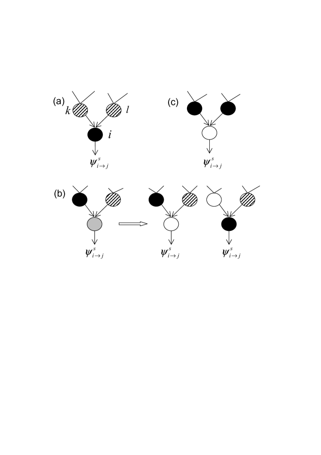
Figure 3: Entropic contribution due to node addition (adding node $i$ and its adjacent links). Each node is connected to $C=3$ nodes. The codes for the cavity probabilities are: shaded for $\psi_{k\rightarrow i}^{s}\in(0,1]$, black for $\psi_{k\rightarrow i}^{s}=0$, white for $\psi_{k\rightarrow i}^{s}=1$ and gray for $\psi_{k\rightarrow i}^{s}\in(0,1)$. The arrow shows the message passing direction. (a) None of the neighbors of node $i$ is frozen to the consumer state in the absence of node $i$. (b) Only one of the neighbors of node $i$, say node $k$, is frozen to the consumer state without node $i$. After the addition of node $i$, it can take the source state or consumer state. (c) At least two of neighbors of node $i$ are frozen to the consumer state in the absence of node $i$.

The value for the cavity probability $\psi_{i\rightarrow j}^{s}$ of node $i$ depends on the incoming cavity probabilities from its neighbors other than node $j$, which can be categorized into three cases.

In the first case as depicted in Fig. 3 (a), all neighbors of node $i$ (other than node $j$) have non-zero cavity probabilities $\{\psi_{k\rightarrow i}^{s}\}$. In this case, the cavity state of node $i$ must be a consumer in the zero temperature limit, and $\Delta F_{i\rightarrow j}=u^{2}/2-\gamma-T\ln\left[\prod_{k\in\partial i\backslash j}\psi_{k\rightarrow i}^{s}\right]$. Hence,

$$\psi_{i\rightarrow j}^{s} =e^{-\beta\gamma-\Delta S_{i\rightarrow j}},$$ (11a)

$$\Delta S_{i\rightarrow j} =\sum_{k\in\partial i\backslash j}\ln\psi_{k\rightarrow i}^{s},$$ (11b)

where $\Delta S_{i\rightarrow j}$ is the cavity entropy change when node $i$ and its adjacent edges except $(ij)$ are added (but the forward link $i\rightarrow j$ is considered in calculating the optimal state).

In the second case (Fig. 3 (b)), only one neighbor of node $i$, say node $k$, is frozen to the c state in the zero temperature limit in the absence of node $i$, i.e., $\psi_{k\rightarrow i}^{s}$ is given by Eq. (11a). Then we have $\Delta F_{i\rightarrow j}=\frac{u^{2}}{2}-T\ln\left[1+e^{-\Delta S_{k\rightarrow i}}\prod_{l\in\partial i\backslash k,j}\psi_{l\rightarrow i}^{s}\right]$, and

$$\psi_{i\rightarrow j}^{s} =\frac{1}{1+e^{-\Delta S_{k\rightarrow i}}\prod_{l\in\partial i\backslash k,j}\psi_{l\rightarrow i}^{s}},$$ (12a)

$$\Delta S_{i\rightarrow j} =\ln\left[1+e^{-\Delta S_{k\rightarrow i}}\prod_{l\in\partial i\backslash k,j}\psi_{l\rightarrow i}^{s}\right].$$ (12b)

The third case where at least two of incoming $\psi_{k\rightarrow i}^{s}$ for node $i$ vanish in the zero temperature limit is presented in Fig. 3 (c). Based on Eqs. (9) and (10), we have

$$\psi_{i\rightarrow j}^{s} =1,$$ (13a)

$$\Delta S_{i\rightarrow j} =0.$$ (13b)

In the above analysis, the added node is assumed to be deficient node. However, a finite fraction of surplus nodes with very large capacities are present in the transportation network as the quenched disorder. The addition of a surplus node is assumed to have no entropy contribution to the network and its full and cavity probabilities are always fixed to be $1$ since it is frozen to the source state by definition. Adding a surplus node will yield different cavity energies depending on the states of its neighbors since the consumer neighbors will draw resources from its adjacent surplus nodes. This leads to the recursive relations $\psi_{i\rightarrow j}^{s}=\delta_{\Lambda_{i},A}+\delta_{\Lambda_{i},-1}\psi_{i\rightarrow j}^{s}|_{\Lambda_{i}=-1}$ and $\Delta S_{i\rightarrow j}=\delta_{\Lambda_{i},-1}\Delta S_{i\rightarrow j}|_{\Lambda_{i}=-1}$, where $\psi_{i\rightarrow j}^{s}|_{\Lambda_{i}=-1}$ and $\Delta S_{i\rightarrow j}|_{\Lambda_{i}=-1}$ are given by the relevant expressions in Eqs. (11) to (13). Note that, if we neglect the entropic effects on the bistable nodes, the above analysis leads to the belief propagation $\psi_{i\rightarrow j}^{s}=\delta_{\Lambda_{i},A}+\delta_{\Lambda_{i},-1}\left[1-\prod_{k\in\partial i\backslash j}\psi_{k\rightarrow i}^{s}\right]$ derived in Ref. Yeung and Wong (2010). Algorithmically, a decimation procedure inspired by the fixed point solution of belief propagation can be devised. We will compare this inspired decimation with the entropic message passing algorithm in Sec. IV.

Figure 4: Sketch for reconnection (a-c) and restoration (d-f) in the cavity iterations. (a) The recursion of the link-headed cavity free energy change given by Eq. (9). (b) The free energy change when node $i$ is reconnected, given by Eq. (16). (c) The free energy change when link $(ij)$ is reconnected, given by Eq. (18). (d) The recursion of the node-headed cavity free energy change, akin to a restoration process, given by Eq. (49). (e) The free energy change when node $i$ and its links are restored, given by Eq. (47). (f) The free energy change when link $(ij)$ is restored, given by Eq. (51).

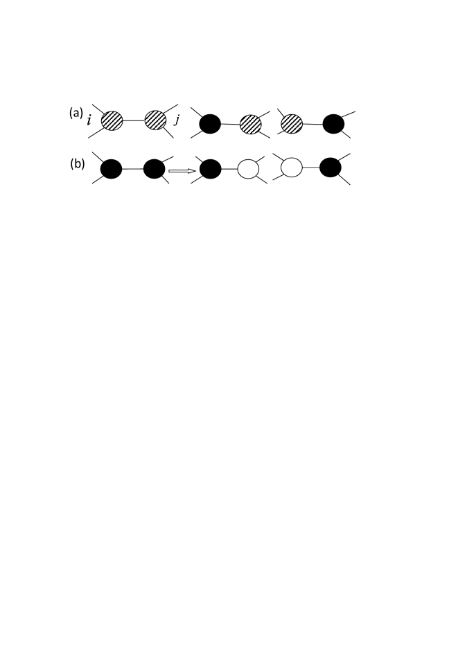
Figure 5: Entropic contribution due to edge addition. The probabilistic meaning for each node is the same as that in Fig. 3. (a) At most one end of the added link is frozen into consumer state before the link addition. (b) Both ends of the added link are frozen into the consumer state in the absence of the link. Then either node $i$ or $j$ should change its state after the link is added.

III.1.2 Disconnecting and reconnecting a node and a link

For a network with $N$ nodes and $L$ links, we consider an initial configuration with $N-1$ nodes and $L$ links, obtained by disconnecting node $i$ from its neighbors, while keeping the links feeding node $i$ dangling in the network. In the dangling links, the flow $x_{ik}$ is considered in optimizing the cavity energy of node $k$ for all $k\in\partial i$. This allows node $k$ to take both the s and c states. Hence the initial free energy is given by

$$F_{N-1,L}=-T\sum_{k\in\partial i}\ln\left(Z_{k\rightarrow i}^{s}+Z_{k\rightarrow i}^{c}\right).$$ (14)

Then we consider the final free energy after the node $i$ is reconnected to its neighbors as shown in Fig. 4 (b). Extending Eq. (8) to include all neighbors of node $i$, we have

$$F_{N,L}=\frac{u^{2}}{2}-T\ln\left[\prod_{k\in\partial i}(Z_{k\rightarrow i}^{s}+Z_{k\rightarrow i}^{c})+e^{\beta\gamma}\prod_{k\in\partial i}Z_{k\rightarrow i}^{s}\right].$$ (15)

Thus the free energy change on reconnecting node $i$ is given by

$$\Delta F_{i}^{{\rm rec}}=\frac{u^{2}}{2}-T\ln\left[1+e^{\beta\gamma}\prod_{k\in\partial i}\psi_{k\rightarrow i}^{s}\right].$$ (16)

Equation (16) is derived by subtracting Eq. (14) from Eq. (15) and using the definition of Eq. (10). The entropy change $\Delta S_{i}^{\rm rec}$ of reconnecting node $i$ can then be computed in the zero temperature limit as

$$\begin{split}\Delta S_{i}^{{\rm rec}}&=\Theta\left(\prod_{k\in\partial i}\psi_{k\rightarrow i}^{s}\right)\sum_{k\in\partial i}\ln\psi_{k\rightarrow i}^{s}+\sum_{k\in\partial i}\left[1-\Theta(\psi_{k\rightarrow i}^{s})\right]\Theta\left(\prod_{l\in\partial i\backslash k}\psi_{l\rightarrow i}^{s}\right)\\ &\times\ln\left[1+e^{-\Delta S_{k\rightarrow i}}\prod_{l\in\partial i\backslash k}\psi_{l\rightarrow i}^{s}\right].\end{split}$$ (17)

The cavity free energy change akin to a reconnection process can be defined according to the link-headed diagrams in Fig. 4 (a). In this case, the cavity free energy change reduces to Eq. (9).

To obtain the entropy contribution of an edge, we consider an initial configuration with $N$ nodes and $L+1$ links, obtained by breaking the link between nodes $i$ and $j$ to form two dangling links, one from node $i$ and the other from node $j$. In the dangling link from node $i$ (node $j$), the flow $x_{ji}$ ($x_{ij}$) is considered in optimizing the cavity energy of node $i$ (node $j$), independent of the cavity energy of node $j$ (node $i$). This allows nodes $i$ and $j$ to take both s and c states. Hence the initial free energy is given by $F_{N,L+1}=F_{i\rightarrow j}+F_{j\rightarrow i}$ where $F_{i\rightarrow j}$ or $F_{j\rightarrow i}$ is given by Eq. (8).

Now we consider the final free energy after reconnecting the link between nodes $i$ and $j$ as shown in Fig. 4 (c). It is more convenient to analyze the free energy change starting from the network with $N-2$ nodes obtained by excluding nodes $i$ and $j$ and all their adjacent links. This includes the following three cases. (a) In both $\partial i\backslash j$ and $\partial j\backslash i$, there are one or more nodes in the c state, then both nodes $i$ and $j$ will be in the s state. No flow is present on the link $(ij)$, and energy change $E_{N}-E_{N-2}=u^{2}$. (b) In either $\partial i\backslash j$ or $\partial j\backslash i$, there are one or more nodes in the c state, and all nodes in the other set are in the s state. In this case, nodes $i$ and $j$ will be in the s and c states (c and s states) respectively. There is a flow from $i$ to $j$ (from $j$ to $i$), and $E_{N}-E_{N-2}=u^{2}-\gamma$. (c) All nodes in $\partial i\backslash j$ and $\partial j\backslash i$ are in the s state. In this case, $i$ and $j$ will be either in the s and c states, or the c and s states respectively. Correspondingly, there is a flow from $i$ to $j$, or from $j$ to $i$, and $E_{N}-E_{N-2}=u^{2}-\gamma$. These three different cases lead to the following free energy change

$$\begin{split}\Delta F_{(ij)}^{{\rm rec}}&=-T\ln\Biggl{[}\left(1-\prod_{k\in\partial i\backslash j}\psi_{k\rightarrow i}^{s}\right)\left(1-\prod_{l\in\partial j\backslash i}\psi_{l\rightarrow j}^{s}\right)+e^{\beta\gamma}\left(1-\prod_{k\in\partial i\backslash j}\psi_{k\rightarrow i}^{s}\right)\prod_{l\in\partial j\backslash i}\psi_{l\rightarrow j}^{s}\\ +&e^{\beta\gamma}\left(1-\prod_{l\in\partial j\backslash i}\psi_{l\rightarrow j}^{s}\right)\prod_{k\in\partial i\backslash j}\psi_{k\rightarrow i}^{s}+2e^{\beta\gamma}\prod_{l\in\partial j\backslash i}\psi_{l\rightarrow j}^{s}\prod_{k\in\partial i\backslash j}\psi_{k\rightarrow i}^{s}\Biggl{]}\\ &+T\ln\left[1+e^{\beta\gamma}\prod_{k\in\partial i\backslash j}\psi_{k\rightarrow i}^{s}\right]+T\ln\left[1+e^{\beta\gamma}\prod_{l\in\partial j\backslash i}\psi_{l\rightarrow j}^{s}\right].\end{split}$$ (18)

We have used Eq. (8) and the definition of the cavity probability $\psi_{i\rightarrow j}^{s}$ in Eq. (10) to derive Eq. (18). Taking the zero temperature limit, we obtain $\Delta S_{\left(ij\right)}=\ln\left[\psi_{i\rightarrow j}^{s}+\psi_{j\rightarrow i}^{s}-\psi_{i\rightarrow j}^{s}\psi_{j\rightarrow i}^{s}\right]$ in cases (a) and (b), which is the entropy change in Fig. 5(a) and $\Delta S_{\left(ij\right)}=\ln\left[e^{-\Delta S_{i\rightarrow j}}+e^{-\Delta S_{j\rightarrow i}}\right]$ in case (c), corresponding to the entropy change in Fig. 5 (b). To sum up, the entropy change due to the link reconnection is written as

$$\begin{split}\Delta S_{\left(ij\right)}^{{\rm rec}}&=\Theta(\psi_{i\rightarrow j}^{s}+\psi_{j\rightarrow i}^{s})\ln\left[1-(1-\psi_{i\rightarrow j}^{s})(1-\psi_{j\rightarrow i}^{s})\right]\\ &+\left[1-\Theta(\psi_{i\rightarrow j}^{s}+\psi_{j\rightarrow i}^{s})\right]\ln\left[e^{-\Delta S_{i\rightarrow j}}+e^{-\Delta S_{j\rightarrow i}}\right].\end{split}$$ (19)

Since the energy in the source location problem is distributed among the installation costs of the nodes and the transportation costs of the links, it is possible to formulate an alternative cavity analysis in which the cavity trees are terminated in nodes instead of links. In this case, changes in the free energy and entropy of a network can be obtained by considering a network with a node or a link first removed and then restored. We call this a restoration process, in contrast to the reconnection process described in this section. Recursion relations and the processes of restoring a node and a link are shown in Fig. 4 (d) to (f) respectively. As derived in Appendix C, subtle differences exist between the two processes, but both processes yield the same results when physical quantities such as the entropy per node are calculated.

III.1.3 Entropy per node

The entropy density of source location problem can be evaluated in the Bethe approximation Mézard and Montanari (2009) through

$$s=\left<\Delta S_{i}\right>-\frac{C}{2}\left<\Delta S_{\left(ij\right)}\right>$$ (20)

where $\left<\cdot\right>$ denotes both the disorder average and the average over the cavity message distribution. The entropy density can be obtained by substituting into Eq. (20) the entropy changes on disconnecting and reconnecting a node and a link (Eqs. (17) and (19)). Remarkably, the result is the same as that obtained by using the zero temperature limit of Eqs. (47) and (51) (removing and restoring a node and a link). This can be seen by noting that the additional terms appearing in Eqs. (48) and (52) cancel each other in Eq. (20).

We evaluate the entropy density by population dynamics algorithm Mézard and Parisi (2001). A population of $\mathcal{N}$ pairs of $(\psi_{i\rightarrow j}^{s},\Delta S_{i\rightarrow j})$ is used to approximate the joint distribution $P(\psi_{i\rightarrow j}^{s},\Delta S_{i\rightarrow j})$ and its components are uniformly updated by the new computed ones according to Eqs. (11) to (13). Usually, a number of iterations $\mathcal{T}-\mathcal{T}_{0}$ are used to compute the entropy value with $\mathcal{T}_{0}$ iterations for equilibration. Note that Eq. (20) gives a self-averaging entropy value in the thermodynamic limit in the sense that the typical value of the entropy computed by the population dynamics algorithm should be consistent with that computed on single large networks Mézard and Montanari (2009).

III.2 One-step replica symmetry breaking analysis

When replica symmetry is broken, the single ground state would break up into exponentially many ground states plus an even larger set of metastable states acting as the dynamical traps for any greedy search algorithm. In this case, one should take into account the reshuffling of free energies of different states when cavity iterations are performed, therefore, we write the replicated free energy $\Phi(y)$ Monasson (1995) as

$$e^{-yN\Phi(y)}\equiv\sum_{\alpha}e^{-yNf_{\alpha}}=\int dfe^{N(\Sigma(f)-yf)}$$ (21)

where $\alpha$ indicates each state and $\Sigma(f)$ is the complexity function counting states with given free energy density $f$. A saddle point analysis of Eq. (21) gives $\Phi(y)=f^{*}-\Sigma(f^{*})/y$ where $f^{*}$ is determined by $y=d\Sigma(f)/df$. The inverse pseudotemperature $y$ allows us to weight differently the various states according to their free energy densities while the usual inverse temperature $\beta=1/T$ selects the energy of equilibrium configurations. Actually, Eq. (21) corresponds to a decomposition of the Gibbs measure Montanari et al. (2008). Here, our analysis is restricted to the ground state ($\beta$ tends to infinity), and $f$ tends to the energy density $\epsilon$ in this limit. For the current problem, the energetic complexity $\Sigma(\epsilon)$ can be computed by the following Legendre transform

$$\Sigma(\epsilon) =y(\epsilon-\Phi),$$ (22a)

$$\epsilon =\frac{\partial(y\Phi)}{\partial y},$$ (22b)

where $\Sigma(\epsilon)$ can be computed from the parametric plot of $\epsilon(y)$ and $\Sigma(y)$ by varying the value of $y$. We remark here that the complexity function of the source location problem vanishes at finite $y$ Yeung and Wong (2010) and this was also observed in studies of the minimal vertex cover problem Weigt and Zhou (2006). Therefore, the Parisi replica symmetry breaking parameter defined by $m=y/\beta$ vanishes in the zero temperature limit. The parameter $m$ is used to select the size of the investigated ground state (entropy), as studied in Refs. Mézard et al. (2005); Zdeborová and Krzakala (2007); Montanari et al. (2008) to compute the entropic complexity curve for random constraint satisfaction problems in the zero ground state energy region and the replicated free energy $\Phi$ reaches the maximum at $y=\infty$(in this case, $m\in[0,1]$ Zhou (2008)).

Due to the proliferation of pure states, we write the recursive equations for the joint distribution $P_{i\rightarrow j}(\psi_{i\rightarrow j}^{s},\Delta S_{i\rightarrow j})$ at the $1$RSB level as

$$\begin{split}P_{i\rightarrow j}(\psi_{i\rightarrow j}^{s},\Delta S_{i\rightarrow j})=\mathcal{Z}_{i\rightarrow j}^{-1}\int\prod_{k\in\partial i\backslash j}dP_{k\rightarrow i}(\psi_{k\rightarrow i}^{s},\Delta S_{k\rightarrow i})e^{-y\Delta E_{i\rightarrow j}}\\ \times\delta\left[\psi_{i\rightarrow j}^{s}-\mathcal{F}(\{\psi_{k\rightarrow i}^{s},\Delta S_{k\rightarrow i}\})\right]\delta\left[\Delta S_{i\rightarrow j}-\tilde{\mathcal{F}}(\{\psi_{k\rightarrow i}^{s},\Delta S_{k\rightarrow i}\})\right]\end{split}$$ (23)

where $dP_{k\rightarrow i}(\psi_{k\rightarrow i}^{s},\Delta S_{k\rightarrow i})\equiv d\psi_{k\rightarrow i}^{s}d\Delta S_{k\rightarrow i}P_{k\rightarrow i}(\psi_{k\rightarrow i}^{s},\Delta S_{k\rightarrow i})$. The functions $\mathcal{F}$ and $\tilde{\mathcal{F}}$ are given by the relevant expressions of $\psi_{i\rightarrow j}^{s}$ and $\Delta S_{i\rightarrow j}$ in Eqs. (11) to (13). The reweighting factor $e^{-y\Delta E_{i\rightarrow j}}$ takes into account the energy change due to cavity operation for the reconnection process (the addition of node $i$, the dangling edge $(ij)$ and the edges to its neighbors other than $j$). Note that $m=0$ makes the contribution of the entropy change in this term disappear. The cavity energy values of $\Delta E_{i\rightarrow j}$ are obtained by the zero temperature limit of Eq. (9), yielding $u^{2}/2-\gamma$ if none of the neighbors $k\in\partial i\backslash j$ takes c state, and $u^{2}/2$ otherwise. Finally, $\mathcal{Z}_{i\rightarrow j}$ is a normalization constant. To simplify the analysis, we parameterize the joint distribution according to the discussion in Sec. III.1 as

$$\begin{split}P_{i\rightarrow j}(\psi_{i\rightarrow j}^{s},\Delta S_{i\rightarrow j})&=p_{i\rightarrow j}^{1}\delta(\psi_{i\rightarrow j}^{s}-1)\delta(\Delta S_{i\rightarrow j})+p_{i\rightarrow j}^{0}\delta(\psi_{i\rightarrow j}^{s})\tilde{\phi}^{0}_{i\rightarrow j}(\Delta S_{i\rightarrow j})\\ &+p_{i\rightarrow j}^{*}\tilde{\phi}^{*}_{i\rightarrow j}(\psi_{i\rightarrow j}^{s},\Delta S_{i\rightarrow j})\end{split}$$ (24)

where $\int d\tilde{\phi}^{0}_{i\rightarrow j}(\Delta S_{i\rightarrow j})=1$, $\int d\tilde{\phi}^{*}_{i\rightarrow j}(\psi_{i\rightarrow j}^{s},\Delta S_{i\rightarrow j})=1$ and $p_{i\rightarrow j}^{1}+p_{i\rightarrow j}^{0}+p_{i\rightarrow j}^{*}=1$. Compared with the RS case where the messages merely consist of the pair $(\psi_{i\rightarrow j}^{s},\Delta S_{i\rightarrow j})$ for each directed edge, here the order parameter turns out to be a survey of these messages at the $1$RSB level; $p_{i\rightarrow j}^{1}$, $p_{i\rightarrow j}^{0}$ and $p_{i\rightarrow j}^{*}$ tell us the probability of picking up a pure state at random and finding that the cavity state of node $i$ is source, consumer and free respectively. These three surveys enable us to handle the state-to-state fluctuations at the $1$RSB level. With this parametric representation, a finite $y$ survey propagation equation can be obtained for the source location problem as

$$p_{i\rightarrow j}^{0} =\delta_{\Lambda_{i},-1}\frac{e^{y\gamma}\prod_{k\in\partial i\backslash j}(p_{k\rightarrow i}^{1}+p_{k\rightarrow i}^{*})}{1+(e^{y\gamma}-1)\prod_{k\in\partial i\backslash j}(p_{k\rightarrow i}^{1}+p_{k\rightarrow i}^{*})},$$ (25a)

$$p_{i\rightarrow j}^{*} =\delta_{\Lambda_{i},-1}\frac{\sum_{k\in\partial i\backslash j}p_{k\rightarrow i}^{0}\prod_{l\in\partial i\backslash j,k}\left(p_{l\rightarrow i}^{1}+p_{l\rightarrow i}^{*}\right)}{1+(e^{y\gamma}-1)\prod_{k\in\partial i\backslash j}(p_{k\rightarrow i}^{1}+p_{k\rightarrow i}^{*})},$$ (25b)

$$p_{i\rightarrow j}^{1} =\delta_{\Lambda_{i},A}+\delta_{\Lambda_{i},-1}(1-p_{i\rightarrow j}^{0}-p_{i\rightarrow j}^{*}).$$ (25c)

After the fixed point of Eq. (25) is obtained, the replicated free energy can be computed via

$$\Phi(y)=\left<\Delta\Phi_{i}\right>-\frac{C}{2}\left<\Delta\Phi_{\left(ij\right)}\right>$$ (26)

where the average is taken over the capacity distribution and the survey distribution, and the replicated free energy shift $\Delta\Phi_{i}$ due to node addition (and its $C$ edges) and $\Delta\Phi_{\left(ij\right)}$ due to link addition are, respectively,

$$-y\Delta\Phi_{i} =\delta_{\Lambda_{i},-1}\left\{-y\frac{u^{2}}{2}+\ln\left[1+(e^{y\gamma}-1)\prod_{k\in\partial i}\left(p_{k\rightarrow i}^{1}+p_{k\rightarrow i}^{*}\right)\right]\right\},$$ (27a)

$$-y\Delta\Phi_{\left(ij\right)} =\ln\Biggl{[}1-(1-e^{-y\gamma})p_{i\rightarrow j}^{0}p_{j\rightarrow i}^{0}\Biggr{]},$$ (27b)

where we have used the energy changes calculated in the zero temperature limits of Eqs. (16) and (18), rather than those of Eqs. (47) and (51). In Eq. (27a), we consider the energy change when node $i$ is reconnected to the network, instead of the change when node $i$ and its links to neighbors are restored to the network. This is because the dangling forward links $i\rightarrow j$ have already been included in the recursion relations of $p_{i\rightarrow j}^{1}$, $p_{i\rightarrow j}^{0}$ and $p_{i\rightarrow j}^{*}$. Similarly in Eq. (27b), we consider the energy change when the dangling forward links $i\rightarrow j$ and $j\rightarrow i$ are reconnected to form the link $(ij)$, instead of the change when link $(ij)$ is restored to the network, since the dangling forward links have already been included in the recursion relations of $p_{i\rightarrow j}^{1}$, $p_{i\rightarrow j}^{0}$ and $p_{i\rightarrow j}^{*}$. The steps involved in this procedure are shown schematically in Fig. 4 (a)-(c).

The energetic complexity can then be computed using Eq. (22). In the glassy phase, $\Sigma(\epsilon)$ typically increases from $y=0$ up to the maximal point forming the first non-physical convex part, yet, with further increase in $y$, decreases down to the zero point where the complexity vanishes at the ground state energy ($y=y^{*}$). This second branch of the complexity curve is the physical concave part Mézard and Parisi (2003). Actually, the zero complexity corresponds to the maximum of the replicated free energy since $\Sigma=y^{2}\partial_{y}\Phi$ from the Legendre transform. To compute the ground state entropy at the $1$RSB level, we should fix $y=y^{*}$.

To derive the formula for the ground state entropy at the $1$RSB level, we first write the replicated free energy $-y\Phi(y,m)=\Sigma(\epsilon,s)-y\epsilon+ms$ keeping a finite value of $m$ Mézard et al. (2005); Zhou (2008) and at the end of the derivation, we get the ground state entropy via $s=\frac{\partial(-y\Phi(y,m))}{\partial m}|_{m=0}$ where $y=y^{*}$ determined by $\Sigma(y^{*})=0$. The $1$RSB approximation of ground state entropy density reads,

$$s =\left<\frac{\left[\Delta S_{i}e^{-y\Delta E_{i}}\right]}{\left[e^{-y\Delta E_{i}}\right]}\right>-\frac{C}{2}\left<\frac{\left[\Delta S_{\left(ij\right)}e^{-y\Delta E_{\left(ij\right)}}\right]}{\left[e^{-y\Delta E_{\left(ij\right)}}\right]}\right>,$$ (28a)

$$\left[\Delta S_{i}e^{-y\Delta E_{i}}\right] =\int\prod_{k\in\partial i}dP_{k\rightarrow i}(\psi_{k\rightarrow i}^{s},\Delta S_{k\rightarrow i})e^{-y\Delta E_{i}}\Delta S_{i}\left(\{\psi_{k\rightarrow i}^{s},\Delta S_{k\rightarrow i}\}\right),$$ (28b)

$$\left[e^{-y\Delta E_{i}}\right] =\delta_{\Lambda_{i},-1}e^{-yu^{2}/2}\left\{1+(e^{y\gamma}-1)\prod_{k\in\partial i}\left(p_{k\rightarrow i}^{1}+p_{k\rightarrow i}^{*}\right)\right\},$$ (28c)

$$\left[\Delta S_{\left(ij\right)}e^{-y\Delta E_{\left(ij\right)}}\right] =\int dP_{i\rightarrow j}(\psi_{i\rightarrow j}^{s},\Delta S_{i\rightarrow j})dP_{j\rightarrow i}(\psi_{j\rightarrow i}^{s},\Delta S_{j\rightarrow i})e^{-y\Delta E_{\left(ij\right)}}\Delta S_{\left(ij\right)},$$ (28d)

$$\left[e^{-y\Delta E_{\left(ij\right)}}\right] =1-(1-e^{-y\gamma})p_{i\rightarrow j}^{0}p_{j\rightarrow i}^{0}.$$ (28e)

Note that in the average $[\cdot]$, $\Delta S_{i}$ and $\Delta S_{\left(ij\right)}$ are still given by RS equations obtained from the zero temperature limits of the free energies in Eqs. (16) and (18) respectively, but the incoming messages to compute them should be sampled from the joint distribution Eq. (24), taking the reweighting factor into account. In addition, $\left<\cdot\right>$ in the first term and second term in Eq. (28a) denote the averages over the capacity distribution and survey distribution and this average can be easily done by the population dynamics algorithm Mézard and Parisi (2001), which yields a typical value of the entropy density.

We remark that the expressions of $\Delta\Phi_{i}$ and $\Delta\Phi_{(ij)}$ obtained in Ref. Yeung and Wong (2010) are different from those in this paper. This is because in Ref. Yeung and Wong (2010), the reweighting factors are based on the cavity free energies following the node-headed recursions in the restoration process schematically depicted in Fig. 4 (d). Hence when $\Delta\Phi_{i}$ and $\Delta\Phi_{(ij)}$ are calculated, Ref. Yeung and Wong (2010) used the free energy changes in Fig. 4 (e) and (f) respectively. However, the finite $y$ survey propagation equation for both reconnection and restoration cases can be verified to be equivalent through an algebraic transformation.

III.3 The appearance of frozen variables as an indicator of $1$RSB, and their distribution

Another way to characterize the glassy behavior is to consider the effects of freezing Boettcher and Percus (2004); Zhou (2005a). We assume the set $\mathcal{D}$ to be dynamical variables (other variables are quenched sources, and treated only as a boundary condition). Frozen variables in our case are those deficient nodes taking the same state (source or consumer) in all ground states. It has been argued that the RSB transition in vertex cover is related to the ability of a quenched variable to induce a long range rearrangement of the ground states Zhou (2005a). In our problem there is a freezing process due to the appearance of long-range correlations related to RSB, but also due to a simple topological element: deficient nodes close to many surplus nodes tend to be frozen simply due to this proximity, independent of the rest of the network. Indeed it is much easier to develop a theory of the latter effect than the former. For this reason it is useful to introduce some (standard) granularity in the network description when discussing freezing.

We consider a subgraph, where only connections amongst dynamical variables are considered. On this subgraph there is a $2$-core, that is the graph that remains after recursively removing dynamical variables of connectivity one or lower. If the thermodynamics of the $2$-core is simple so is the entire graph, variables outside the $2$-core are in tree like structures that cannot exhibit a RSB behavior independently of the $2$-core.

Let us consider the ensemble of regular $C=3$ random graphs with a fraction ($1-\phi_{s}$) of deficient nodes, as later studied numerically. We can further refine our definition of deficient nodes on the $2$-core: those nodes of connectivity $3$ we call hubs, and those of connectivity $2$ non-hubs. The simplest case is $\phi_{s}=0$, in which the entire graph is the $2$-core, and all variables are hubs (but this is the exception). By contrast when $\phi_{s}>\frac{1}{C-1}$, the quenched nodes are so numerous that the dynamical variables become disconnected in components of size $o(N)$, that is the $2$-core disappears and there are no hubs. The fraction of hubs in the $2$-core can be calculated analytically by the following procedure. First, we define a probability $p_{dd}$ that a deficient node in the $2$-core is dangling (of connectivity $1$), and this happens only when the states for $C-1$ of its neighbors are either surplus or dangling deficient. Thus $p_{dd}$ satisfies the recursive equation $p_{dd}=\left[\phi_{s}+(1-\phi_{s})p_{dd}\right]^{C-1}$, whose stable fixed point is denoted as $p_{dd}^{*}(=\phi_{s}^{2}/(1-\phi_{s})^{2}$ for $C=3$). A deficient node is a hub only when all of its $C$ neighbors are neither surplus nor dangling deficient, therefore the fraction of hubs in the $2$-core is $f_{{\rm hubs}}=(1-\phi_{s})\left[(1-\phi_{s})(1-p_{dd}^{*})\right]^{C}$. For $C=3$, we have

$$f_{{\rm hubs}}=\frac{(1-2\phi_{s})^{3}}{(1-\phi_{s})^{2}}.$$ (29)

The hubs can be loosely considered as those nodes furthest from the surplus nodes, but also control the phenomena of freezing. Let us consider for example a system in which all hubs are quenched to particular values (frozen and inflexible). Now if any non-hub is quenched to a particular value, will it cause an extensive rearrangement of the ground states? The freezing of the hubs indicates that this propagation would be restricted to only a short chain within the $2$-core, and terminate at the nearest hubs. This indicates the phenomenological importance of the hubs. In order for information from the quenched variable to propagate effectively, there must exist a freedom of hubs to change state and thereby branch the information outward. Of course frozen hubs can be perturbed if we allow for a change in energy, the range of propagation of information would then depend on the nature of the freezing—if the freezing is caused by proximity to a boundary, there will again be no long range reordering, whereas if the freezing happens in a graph-wide correlated manner, there will be a long range reordering of the system that is typical of RSB.

III.4 Population dynamics

We evaluate the entropy numerically by population dynamics algorithm. At the $1$RSB level, we create a population of $\mathcal{N}$ pairs of $(p_{i\rightarrow j}^{0},p_{i\rightarrow j}^{*})$ with an additional population of $\mathcal{M}$ pairs of $(\psi_{i\rightarrow j}^{s},\Delta S_{i\rightarrow j})$ associated with each element of the first population. Elements of both populations are updated in the population dynamics iterations. A number of iterations $\mathcal{T}-\mathcal{T}_{0}$ are used to compute the entropy value with $\mathcal{T}_{0}$ iterations for equilibration. Another relevant quantity is the fraction of source nodes $f_{s}$ in the final optimized network. Its typical value can be evaluated as $f_{s}=\frac{1}{N}\sum_{i=1}^{N}\left<\psi_{i}^{s}\right>$ at the RS level or $1$RSB level. The average is taken over the disorder and the RS message or $1$RSB survey distribution, and $\psi_{i}^{s}$ is the full or marginal probability given by $\psi_{i}^{s}=\delta_{\Lambda_{i},A}+\psi_{i}^{s}|_{\Lambda_{i}=-1}$ where $\psi_{i}^{s}|_{\Lambda_{i}=-1}$ is determined by Eq. (11a), (12a) and (13a) in which $\partial i\backslash j$ is replaced by $\partial i$.

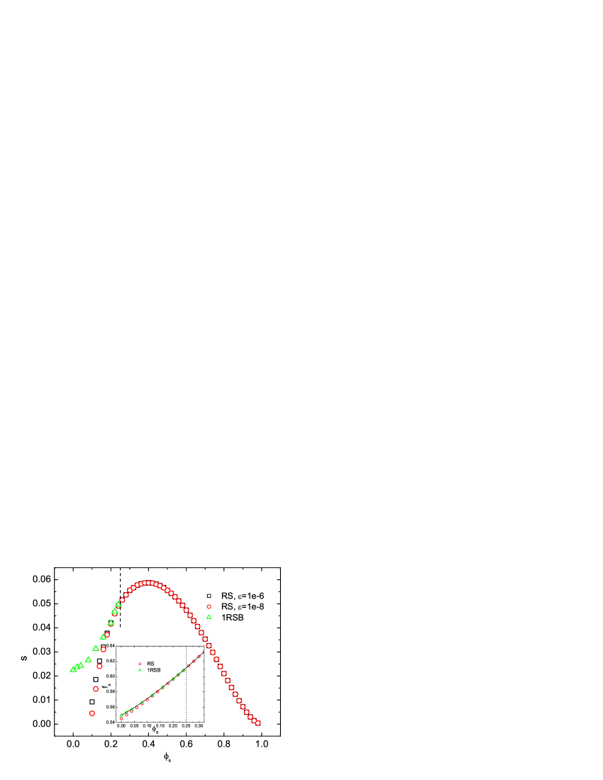
Figure 6: (Color online) Ground state entropy density versus the fraction of surplus nodes $\phi_{s}$. The vertical dashed line indicates the dynamical transition below which the RS description becomes incorrect. The RS results are obtained using different cutoffs $\varepsilon=10^{-6}$ and $10^{-8}$. The network parameter $C=3$ and the population size for RS computation is $\mathcal{N}=10^{5}$, and $(\mathcal{N},\mathcal{M})=(2048,1024)$ for $1$RSB computation. The inset gives the typical ground state fraction of source nodes in the final optimized network. The solid line is the asymptotic limit obtained by EO.

In the following studies, we choose $u=2/3$ and $C=3$ which fall within the range of the singlet regime $1/\sqrt{C}<u<\sqrt{(C+1)/[C(C-1)]}$ Yeung and Wong (2010). The entropy values of the ground state at both RS and $1$RSB levels are given in Fig. 6. We use $(\mathcal{T},\mathcal{T}_{0})=(5000,1000)$ for RS computation and $(\mathcal{T},\mathcal{T}_{0})=(1500,500)$ for $1$RSB computation. Only the mean value of the entropy density is plotted since the error bar is much smaller than the symbol size. In the RS population dynamics, the extremely small value for certain cavity probabilities can be observed when $\phi_{s}$ is sufficiently small, and this is equivalent to the divergence of the evanescent cavity fields Huang and Zhou (2009); Zhang et al. (2009). However, if we take a proper cutoff $\varepsilon$ for the nearly vanishing probability, this situation can be circumvented Zhou and Zhou (2009) and the resulting entropy value seems to be insensitive to the cutoff value as long as $\varepsilon\geq 10^{-6}$ in the stable region of RS solution. For the $1$RSB computation, we adopt $\varepsilon=10^{-6}$ (smaller values of $\varepsilon$ do not change much the result). In Fig. 6, the entropy density first increases when $\phi_{s}$ decreases, then reaches a maximum followed by the decreasing trend as the fraction of surplus nodes (disorder) further decreases. At a large value of $\phi_{s}$, most nodes are surplus nodes, the entropy should take a small value; when $\phi_{s}$ gets close to zero, most nodes are deficient nodes, which makes the source locations much more constrained and yields a small value of entropy. Due to the concavity of the entropy function, there should exist some maximum point and this point can be identified by the mean field computation in Fig. 6. The maximum implies that at the corresponding $\phi_{s}\simeq 0.40$, there exists the largest number of optimal assignments satisfying the singlet connection pattern among all values of $\phi_{s}$.

At $\phi_{s}=0.25$, the replica symmetric solution starts to be unstable against $1$RSB perturbations Yeung and Wong (2010). This is confirmed by the fact that above this transition point, the complexity calculated by $1$RSB equations (25) does not depend on the value of $y$ and is always zero, while it has a finite value below the transition point. This transition point is also called the dynamical transition threshold below which the local search process is usually trapped by the metastable states. For the source location problem, the replicated free energy reaches its maximum at finite $y$ and actually the maximum corresponds to the ground state Mézard and Parisi (2003). In the zero temperature limit, one can thus obtain the ground state energy. Within the current context, the ground state entropy value in the $1$RSB ansatz can also be computed improving the RS prediction. We also show the fraction of source nodes in the ground state in the inset of Fig. 6 where the $1$RSB ansatz predicts a higher value compared with the RS ansatz. The $1$RSB result is consistent with the asymptotic limit obtained by EO (see Sec. III.5). We compute $f_{s}$ through the linear relationship $f_{s}=(\epsilon-1/(2C)+\phi_{s}u^{2}/2)/\gamma$ since we have the identity $(1-f_{s})/(2C)+(f_{s}-\phi_{s})u^{2}/2=\epsilon$. In this sense, the $f_{s}$ serves as a measure of the ground state energy density. These values will be compared with those obtained from simulations on single instances in Sec. IV. As shown in the inset of Fig. 6, $f_{s}$ decreases as $\phi_{s}$ decreases. Actually, one deficient node causes an installation cost ($u^{2}/2$) when converted to a source node while it leads to an increment of $1/(2C)$ of the transportation cost when remaining as a consumer node. Notice that the consumer state is energetically favored since $\gamma>0$ in the singlet regime. Consequently, on one hand, as $\phi_{s}$ decreases, the number of deficient nodes increases, on the other hand, to yield the minimal energy cost, some deficient nodes need to remain as consumer nodes while consumer nodes are not allowed to be paired in the singlet regime. The competition of these two effects leads to the decreasing trend of $f_{s}$ with decreasing $\phi_{s}$.

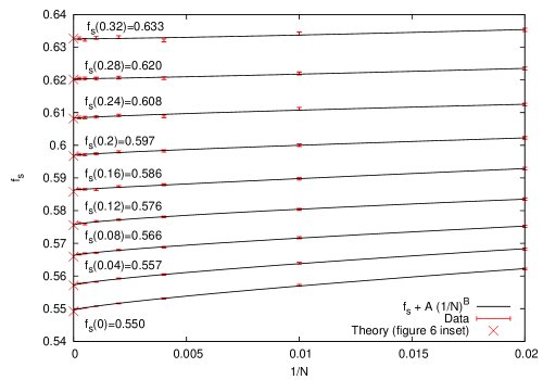
Figure 7: (Color online) Ground state energy achieved by EO. A power law fitting as $f_{s}(N,\phi_{s})=f_{s}(\phi_{s})+AN^{-B}$ is applied. For $\phi_{s}>0.25$, $B\simeq 1.0$, however, $B$ decreases to a value $\simeq 0.8$ for $\phi_{s}$ close to zero.

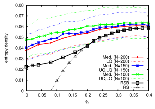
Figure 8: (Color online) The medians and upper and lower quartiles (Med, UQ and LQ) for the entropy distribution for a set of $1500$, $1000$ and $500$ graphs for $N=100$, $150$ and $N=200$ respectively. For $N=200$ the entropy becomes very large, meaning that only the median and lower quartile can be established.

III.5 Numerical verification by extremal optimization

Extremal Optimization (EO) is a local stochastic search method that has been employed successfully to understand the ground-state properties of spin-glass like systems Boettcher (2003a); Boettcher and Percus (2004); Raymond and Wong (2012). It succeeds by searching with a scale-free rule for changing states, in such a way that it reaches low energy states, but is not trapped by large energy barriers typical of systems that exhibit RSB behavior. In this paper it is employed to experimentally verify the energy and entropy of the singlet regime, as well as to investigate freezing properties. The implementation details of this procedure are shown in Appendix D. EO has been used to study the average ground state energy, backbone, entropy and local field distribution of spin glass models Boettcher (2003a, b); Boettcher and Percus (2004); Boettcher et al. (2008). Our use of EO in the exploration of extensive entropic properties is a new application, but can be justified along the same lines as previous studies: we know that EO will not sample uniformly the ground states, however to establish the entropy we need only count the ground states for which a biased sampler can be suitable as explained in the Appendix D and justified empirically.

Data from various system sizes can be combined to estimate asymptotic result and quantify finite size effects, as plotted in Fig. 7. We have fitted a curve of the form $f_{s}(N,\phi_{s})=f_{s}(\phi_{s})+AN^{-B}$, to our energy data, where $f_{s}(\phi_{s})$ is our estimate of the asymptotic ground state energy. Using the Marquardt-Levenberg method to fit the data, we acquire the curves in Fig. 7 in which the error bars associated to the sample mean are plotted, from which the limiting values are obtained with errors smaller than $10^{-3}$ in every case. The exponent $B$ varies from approximately $0.785\pm 0.025$ at $\phi_{s}=0$, to statistically indistinguishable from linear ($B\simeq 1.0$) for $\phi_{s}\gtrsim 0.25$. The asymptotic limit $f_{s}(\phi_{s})$ shown in the plot is consistent with the theoretical prediction in Fig. 6 (inset). Fig. 8 shows the entropy obtained by EO as described in Appendix D. The quartiles and medians of the statistics indicate a broad range of entropies. For low $\phi_{s}$ , especially in the glassy region described by RSB, the median curves of the EO statistics appear to approach a limiting curve from above. However, the combination of lower quartile and median curves indicates there may be a significant gap to the $1$RSB theory. Given the network size less than $200$, this may be due to finite size effects, or may be related to higher order RSB corrections. Since the numerical method employed involves recording and comparing all ground states, we are restricted to studying systems of size $N\lesssim 200$. The data, in particular the lower quartile curve, indicates a concentration of the entropy at an extensive value, in qualitative agreement with the $1$RSB result for smaller $\phi_{s}$, and in quantitative agreement with RS and $1$RSB for larger $\phi_{s}$, which furthermore confirms that $1$RSB becomes a better approximation than RS in the low $\phi_{s}$ regime.

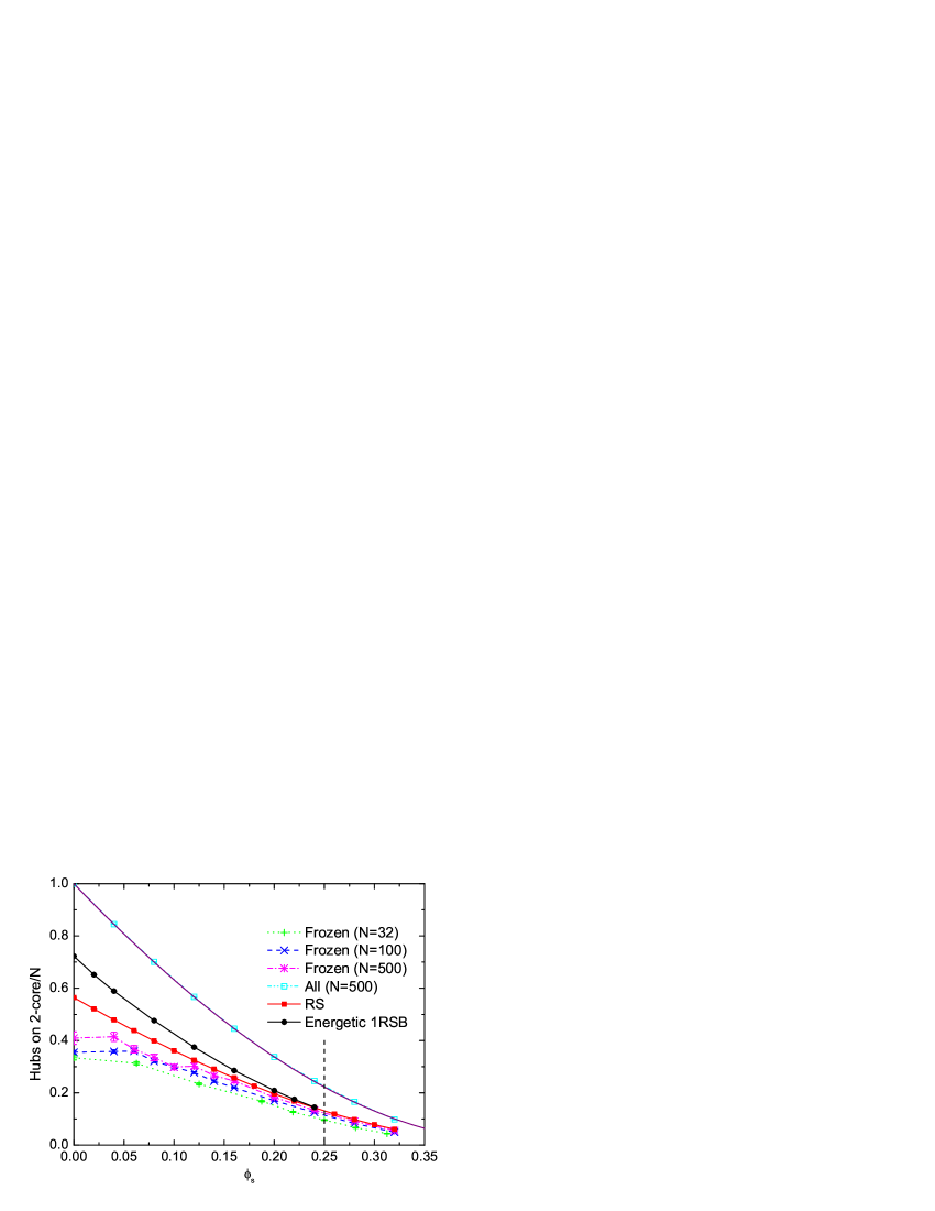
Figure 9: (Color online) Statistics of hubs on $2$-core versus the quenched disorder $\phi_{s}$. The upper solid line is the analytic prediction for the fraction of hubs on $2$-core. It predicts the numerical data on graphs of $N=500$ very well. The vertical dashed line indicates the dynamical transition point. The freezing phenomena is predicted well for $\phi_{s}\gtrsim 0.12$, at which point there is a deviation between the theory and numerical results.

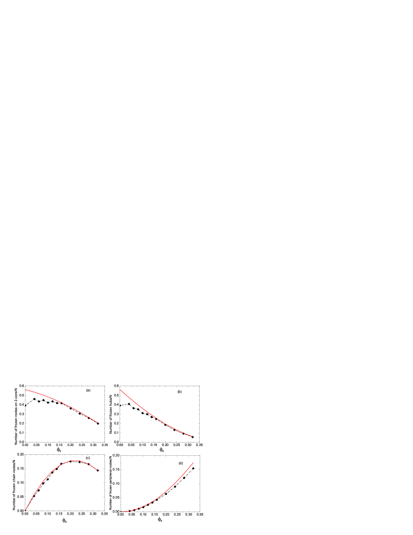
Figure 10: (Color online) The dependence of the fraction of frozen nodes on the fraction $\phi_{s}$ of surplus nodes. (a) All frozen $2$-core nodes considered. (b) Frozen hubs. (c) Frozen chain nodes. (d) Frozen peripheral nodes. Lines: RS prediction. Symbols: Results obtained by the EO algorithm, extrapolated linearly to the infinite size limit (based on data at $N=50,100,250,500$ and $1000$ with $2500,2500,1000,240$ and $60$ samples respectively).

The effect of freezing can also be probed with the EO numerical method (see Appendix D). Fig. 9 shows the mean density of hubs and density of frozen hubs (based on $2500,2500,240$ samples for graphs of $N=32,100,500$ respectively). We also plot the entropic RS prediction and energetic $1$RSB prediction for the frozen hubs in Fig. 9. The numerical data for high $\phi_{s}$ is consistent with the theoretical prediction, while for small $\phi_{s}$ the numerical results continue to evolve rapidly with $N$ towards the theoretical curves from below. We find that the $1$RSB theory predicts a higher value of the fraction of frozen hubs after the dynamical transition than RS. However, the theoretical prediction of the fraction of frozen hubs is higher than that measured in numerical experiments when replica symmetry is broken. This is because the theoretical prediction calculates the expected value of the fraction of frozen nodes in one (or a few) dominant pure state, whereas, the landscape at the system sizes studied by the EO algorithm has important finite size effects and strong sample to sample fluctuations. We propose an argument that could explain the convergence of the numerical results to the theoretical ones from below: In many samples, additional minima that would be negligible asymptotically are captured by EO, moreover, each minimum is significantly distant from the other minima, and so unfreezes a significant fraction of variables which are initially frozen in the dominating minima (that we expect to agree with the theory). This may also be one of reasons for the inconsistency of entropy values between theory and EO statistics at low $\phi_{s}$ in Fig. 8. The numerical results for the density of frozen variables approximately agree with the RS prediction when the RS entropy in Fig. 6 remains positive, but deviate significantly from theory in the strongly constrained regime, where the RS entropy becomes negative.

The effects of frozen hubs on the breakdown of the RS prediction are further illustrated in Fig. 10. We classify the deficient nodes in the network into $2$-core nodes and peripheral nodes (those that are not on $2$-core). Figure 10 (a) and (d) show that the fraction of $2$-core nodes deviates from the RS prediction when $\phi_{s}$ is small, whereas the fraction of frozen peripheral nodes is almost consistent with the RS prediction in the entire range of $\phi_{s}$. Among the $2$-core nodes, we further classify the deficient nodes into hubs (those connected to $3$ other $2$-core nodes) and chain nodes (non-hubs connected to only $2$ other $2$-core nodes) and compare their behaviors in Fig. 10 (b) and (c). We conclude that the deviation from the RS prediction is primarily attributed to the hubs rather than other substructures as shown in Fig. 10. There is freezing close to the quenched boundary, which is due to local RS-like features, and freezing on the core that relates to the graph-wide RSB phenomena; the latter becomes increasingly important as $\phi_{s}$ decreases. The strong deviation from theory indicates that optimization problems with quenched disorder, as analyzed in this paper, could provide an alternative test of theories of the relationship between the freezing and the RSB transition Zhou (2005a); Wei et al. (2012).

IV Numerical studies on single instances

In this section, we apply the entropic message passing approach derived in Sec. III.1 to study single instances of networks. Two kinds of decimation strategy are used to identify the optimal source location. One strategy is the maximal decimation in which the most polarized nodes are fixed once the algorithm converges and then the network is simplified correspondingly. This strategy can be thought as a hard decimation since it is equivalent to adding an external field of infinite intensity to the decimated nodes Braunstein et al. (2005); Montanari et al. (2007); Ricci-Tersenghi and Semerjian (2009). The other is the reinforcement strategy which can be viewed as a sort of soft decimation. In this strategy, the cavity probability is strengthened or attenuated at each step by an external bias whose intensity is updated with a rate increasing with the run time Chavas et al. (2005); Dall’Asta et al. (2008); Zdeborová and Mézard (2008). When the updating rate and the intensity of the external bias are correctly chosen, the external messages are able to drive the iterations towards some optimal assignment thanks to the fact that this soft decimation utilizes the global information of the network at each step. The belief propagation inspired decimation is also compared. Hereafter, we use the short-hand notations BPD for belief propagation inspired decimation, EMPD for entropic message passing inspired decimation and EMPR for entropic message passing reinforcement algorithm.

IV.1 Maximal decimation strategy

For the maximal decimation strategy, we fix a fraction $f_{d}$ of $N_{t}$ unfixed nodes with the largest full probability $\psi_{i}^{s}$ to their most probable states once the algorithm converges at the $t$-th sweep ($f_{d}=2\%$ in our simulations). Each sweep consists of a sequential update of the messages on all the edges of the network in a random order. When $f_{d}N_{t}<1$, only one node with the largest bias is fixed. In the glassy phase, the algorithm typically fails to converge, and this is due to the building up of the long range correlations of different parts of the network. Therefore, we carry out the decimation according to the time-averaged full probability (over a number of sweeps) instead of the instantaneous value of the probability Bounkong et al. (2006). When a node, say $i$ is fixed, the network is simplified by the following decimation procedure. If the node is fixed to the source state, it will send out the message $\psi_{i\rightarrow j}^{s}=1$ to all its neighbors $j\in\partial i$ regardless of the later recursions. Otherwise, all neighbors of node $i$ should take source state and are fixed at the same time since no paired consumer nodes are allowed in the singlet regime. Correspondingly, these fixed source nodes send out a constant message $\psi_{i\rightarrow j}^{s}=1$ to their neighbors. However, if at least one of neighbors of node $i$ has been fixed to consumer in this case, a contradiction will be reported and we restart the algorithm. After the decimation, the recursion is carried out on the unfixed nodes of the network until $N_{t}=0$ and an optimal assignment of source location is obtained. One can compute the marginal probability either based on the belief propagation $\psi_{i\rightarrow j}^{s}=\delta_{\Lambda_{i},A}+\delta_{\Lambda_{i},-1}\left[1-\prod_{k\in\partial i\backslash j}\psi_{k\rightarrow i}^{s}\right]$ derived using the energetic cavity method, or according to the entropic message passing equations derived in Sec. III.1. The pseudocode of EMPD is given as follows:

 
EMPD algorithm
INPUT: the network with a fraction $\phi_{s}$ of surplus nodes; a maximal number of iterations $T_{max}$; a predefined precision $\eta$.
OUTPUT: one assignment in the singlet regime or ’probably no solutions’.

• Initialize randomly $\psi_{i\rightarrow j}^{s},\Delta S_{i\rightarrow j}$ for all edges of the network except for the edges connected to the surplus nodes;

• for $t=1$ to $t=T_{max}$ do:

  • a sweep of random sequential update of the messages $\{\psi_{i\rightarrow j}^{s},\Delta S_{i\rightarrow j}\}$ for all edges according to Eqs. (11), (12) and (13);

  • if $|\psi_{i\rightarrow j}^{s}(t)-\psi_{i\rightarrow j}^{s}(t-1)|<\eta$ and $|\Delta S_{i\rightarrow j}(t)-\Delta S_{i\rightarrow j}(t-1)|<\eta$ for all edges and the iteration has converged: goto line 3;

• if $t<T_{max}$, compute the full probability $\psi_{i}^{s}$ for unfixed nodes and decimate the network, else do the time average of the full probability over the later $T_{max}/2$ sweeps and decimate the network;

• if an optimal assignment is found, return the solution and stop; else if no contradiction is found, continue the decimation procedure on the smaller network (goto line 2); else if a contradiction is meet, return ’probably no solutions’ and stop.

 

IV.2 Soft decimation strategy

The reinforcement strategy has been used to find solutions for random constraint satisfaction problems Chavas et al. (2005); Dall’Asta et al. (2008); Zdeborová and Mézard (2008). Here, we introduce an external bias $\mu_{i}$ for each node, and its intensity is updated with a probability increasing with the running time as $1-t^{-r}$. The external bias $\mu_{i}$ is updated as $\mu_{i}=\pi$ if $\psi_{i}^{s}<0.5$ and $1-\pi$ otherwise. The bias strength $\pi\in[0,0.5]$. This implies that the current value of the cavity probability of one node will be enhanced by a factor if its full probability at the preceding iteration is biased towards the source state. Thus the only modification to the original recursive equation Eqs. (11a), (12a) and (13a) is

$$\tilde{\psi}_{i\rightarrow j}^{s}=\frac{\mu_{i}\psi_{i\rightarrow j}^{s}}{\mu_{i}\psi_{i\rightarrow j}^{s}+(1-\mu_{i})(1-\psi_{i\rightarrow j}^{s})}$$ (30)

where $\tilde{\psi}_{i\rightarrow j}^{s}$ is the reinforced cavity probability while $\psi_{i\rightarrow j}^{s}$ is the original one computed from Eqs. (11a), (12a) and (13a). Both $\pi$ and $r$ should be optimized so as to properly guide the iteration to converge to an optimal assignment. In the numerical simulation, we fix $r=0.1$ although other choices also lead to find a solution, e.g., $r=0.3$. The algorithm is precisely described as follows:

 
EMPR algorithm
INPUT: the network with a fraction $\phi_{s}$ of surplus nodes; a maximal number of iterations $T_{max}$; two empirical parameters $\pi$ and $r$.
OUTPUT: one assignment in the singlet regime or ’probably no solutions’.

• Initialize randomly $\psi_{i\rightarrow j}^{s},\Delta S_{i\rightarrow j}$ for all edges of the network except for the edges connected to the surplus nodes and initialize the external biases $\{\mu_{i}\}$ at random;

• for $t=1$ to $t=T_{max}$ do:

  • a sweep of random sequential update of the messages $\{\psi_{i\rightarrow j}^{s},\Delta S_{i\rightarrow j}\}$ for all edges according to Eqs. (11), (12), (13) and Eq. (30);

  • update all the external biases with probability $1-t^{-r}$;

  • assign $s_{i}=1$ if $\mu_{i}>0.5$ and $0$ otherwise; if $\{s_{i}\}$ is an optimal assignment (no contradiction), return the solution and stop.

• if $t=T_{max}$, return ’no solutions at current values of $\pi$ and $r$’.

 

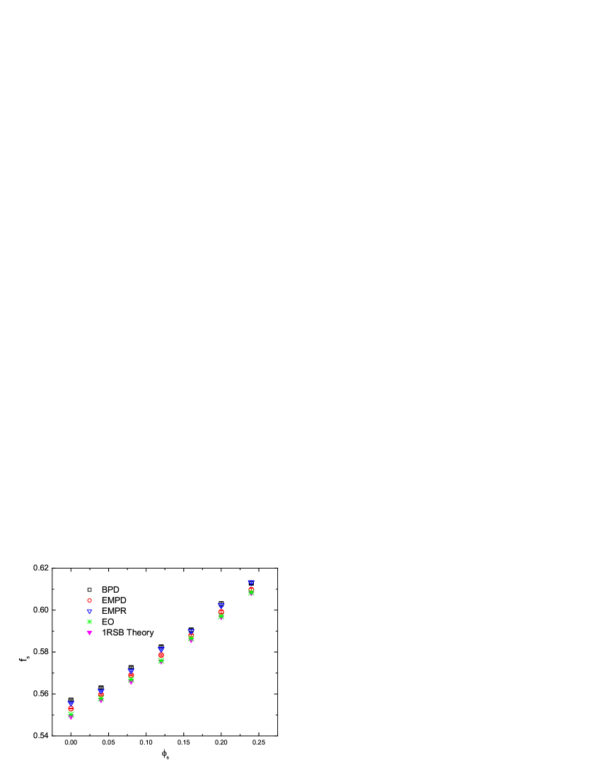
Figure 11: (Color online) The fraction of source nodes in the optimized network ($N=2000$) obtained by different algorithms. For BPD and EMPD, $f_{d}=2\%$, $T_{max}=2000$ and $\eta=10^{-3}$ and additionally for EMPD, $\varepsilon=10^{-6}$. $T_{max}=10^{4}$ for EMPR. $\tau=1.8$ for EO. The data point is the mean over $30$ random regular networks with $C=3$ and the error bar is also shown.

The inference results using the above proposed algorithms on single instances of size $N=2000$ are compared in Fig. 11. BPD has been compared with GSAT algorithm which randomly selects a small cluster of nodes and then update its configuration to the one with lowest network energy, however, GSAT yields a higher energy Yeung and Wong (2010). As shown apparently in Fig. 11, the entropic message passing algorithm yields a lower value of $f_{s}$ than the belief propagation without taking the entropic effects into account, and hence achieves a more optimal cost. Its value is also closer to the theoretical $1$RSB prediction. This indicates the advantages of employing entropic information in message passing procedure to differentiate states that are locally ambiguous but possibly lead to frustrations in the long range.

It should be mentioned that EMPR can find the optimal assignments faster than other strategies in the glassy regime. This is because, on the one hand, the presence of an updating external bias manages to drive the evolution of the reinforced cavity probabilities towards the ground state where the satisfying assignment is maximally aligned with the externally imposed direction; on the other hand, the hard decimation fails to converge in this regime and the time-average of the marginal probabilities is required, which increases the time complexity of the algorithm. In the RS region, EMPR becomes slow because the proper values of $(\pi,r)$ could not be easily found, probably due to the presence of the many background messages sent out by the surplus nodes. In contrast, the EMPD and BPD are typically convergent in this regime and thus fast to identify the optimal assignment. In the glassy regime, the estimated $f_{s}$ by message passing algorithms is higher than the ground state value predicted by the $1$RSB theory. The physical interpretation is, in the glassy region, exponentially many metastable states act as dynamical arrests for various simple heuristics. Furthermore, the ground state predicted by the $1$RSB theory can be unstable towards further steps of RSB or full RSB (an infinite hierarchy of nested states) Yeung and Wong (2010); Mézard and Montanari (2009), and the lower bound to the true dynamical threshold of $f_{s}$ is predicted by the Gardner value Gardner (1985) above which the $1$RSB metastable states become unstable Montanari et al. (2004). However, the entropic message passing algorithm on single instances yields a lower value of $f_{s}$, and particularly the EMPD can give a lowest value of $f_{s}$ among all message passing algorithms in the glassy region. Note that the attained energy can be further lowered for the hard decimation by taking smaller $f_{d}$ at the expense of larger computational time. We also put the inference result by EO algorithm (see Appendix D) in Fig. 11. The time complexity for EO to find a ground state is of the order $\mathcal{O}(N^{3})$ while the hard decimation converges in $\mathcal{O}(N^{2})$ when fixing at each step only one variable and the soft decimation converges in the order of $\mathcal{O}(N)$. When we fix a given fraction of variables at each step, the time complexity for the hard decimation reduces to be of the order $\mathcal{O}(N\ln N)$.

V Conclusion

We have considered the entropic effects in the ground state of the source location problem and derived the associated entropic message passing algorithms as an improvement over the previous energetic computation of the problem. Using the $1$RSB ansatz, the ground state entropy predicted by the RS solution is improved and yields a better approximation. Although the formula for the entropy in the RS ansatz is equivalent to that of the minimal vertex cover problem, computation of the entropy in the $1$RSB ansatz requires additional energetic information different from that in the vertex cover problem. In particular, the energy changes we used to compute the entropy values in the $1$RSB case include the influence of the forward links, which is necessary for the case where flows on the links also contribute to the energy. We found that the $1$RSB recursions can be computed in a way similar to that in Ref. Yeung and Wong (2010) which did not consider the entropy but only the energy, but by carefully monitoring the free energy changes due to restoration and reconnection of nodes and links, we found an alternative derivation. This also provides tools to analyze network optimization problems dependent on both node and link conditions.

The predicted $f_{s}$ are checked by the simulations on single instances of transportation networks. Using the message passing inspired decimation algorithms, we find that the entropic information helps to lower the inference value of $f_{s}$ making it closer to the ground state value. This advantage is due to the extra information gained from entropy considerations guiding us to choose one of the two possible bistable states correctly and hence resolve potential conflicts arising from long-range frustrations.

The theoretical results of ground state energy agree with those obtained independently by the EO method. However, the agreement of the entropy value at low $\phi_{s}$ is less satisfactory. Large finite size effects and strong sample-to-sample fluctuations are present. We also found that the entropy is extensive when the RS prediction becomes unstable, matching theoretical predictions in the $1$RSB framework. By studying the fraction of frozen nodes according to their topological classification, it was revealed that frozen hubs are the primary cause for the breakdown of the RS prediction in its unstable regime. On the technical aspect, large size measurements of frozen set of variables and entropies are useful in understanding the RSB phenomena, but the sampling of ground states is numerically challenging.

As the installation cost parameter $u$ increases, another important configuration of source and consumer nodes, namely the doublet regime will appear. Extension of the current method to this regime would be very interesting. In this case, to derive the recursive equations, we need to define two extra cavity messages, one for singly consuming state and the other for doubly consuming state. Due to many more ways of clustering the consumer nodes, we anticipate that entropic effects will be very significant at the commensurate points in the doublet regime Yeung and Wong (2010). The present work has established the foundation, and one can extend the analysis by including one more term for the doubly consumer state in the free energy expression. It is also of interest to extend the current analysis to the lattice glass models Biroli and Mézard (2002); Rivoire et al. (2004) where for example each site in the (finite dimensional or Bethe) lattice can have at most one particle and any particle has at most a fixed number of occupied nearest neighbor. Other possible applications may be found in routing and path selection problems on sparse graphs Yeung and Saad (2012).

Appendix A Cavity analysis of the model

Here we briefly present a theoretical analysis of the model defined in Eq. (3) based on the cavity method Mézard and Montanari (2009) and finally demonstrate its relation to the minimal vertex cover problem. The original derivation was given in Ref. Yeung and Wong (2010).

The network we consider here has a locally tree-like structure, as described in Fig. 2 or Fig. 3. We define $E_{i\rightarrow j}(x_{ji})$ as the cavity energy of the tree terminated at node $i$ without consideration of its ancestor node $j$, and $E_{i\rightarrow j}(x_{ji})$ is determined by

$$\begin{split}E_{i\rightarrow j}(x_{ji})&=\mathcal{E}(E_{k_{1}\rightarrow i},E_{k_{2}\rightarrow i},\ldots,E_{k_{C-1}\rightarrow i};\Lambda_{i},x_{ji})\\ &\equiv\min_{\{x_{ik}\}}\left[\sum_{k\in\partial i\backslash j}E_{k\rightarrow i}(x_{ik})+\frac{u^{2}}{2}\Theta\left(-\Lambda_{i}-\sum_{k\in\partial i\backslash j}x_{ik}+x_{ji}\right)+\frac{x_{ji}^{2}}{2}\right],\end{split}$$ (31)

in the zero-temperature limit. The first term sums over all energies of descendants, while the second and last terms refer to the penalty for negative final resource and transportation cost respectively. To write a recursion of an intensive energy, we separate the extensive quantity $E_{i\rightarrow j}(x_{ji})$ into two terms:

$$E_{i\rightarrow j}(x_{ji})=E_{i\rightarrow j}^{V}(x_{ji})+E_{i\rightarrow j}(0),$$ (32)

where $E_{i\rightarrow j}^{V}(x_{ji})$ is called a vertex-dependent intensive energy such that $E_{i\rightarrow j}^{V}(0)=0$. In fact, $E_{i\rightarrow j}^{V}(x_{ji})$ describes the energy variation from $E_{i\rightarrow j}(0)$ as $x_{ji}$ changes. This allows us to recast Eq. (31) into

$$E_{i\rightarrow j}^{V}(x_{ji})=\mathcal{E}(E_{k_{1}\rightarrow i}^{V},E_{k_{2}\rightarrow i}^{V},\ldots,E_{k_{C-1}\rightarrow i}^{V};\Lambda_{i},x_{ji})-\mathcal{E}(E_{k_{1}\rightarrow i}^{V},E_{k_{2}\rightarrow i}^{V},\ldots,E_{k_{C-1}\rightarrow i}^{V};\Lambda_{i},0).$$ (33)

From the above definition, one arrives at the energy change due to addition of a node:

$$\Delta E_{{\rm node}}=\mathcal{E}(E_{k_{1}\rightarrow i}^{V},E_{k_{2}\rightarrow i}^{V},\ldots,E_{k_{C}\rightarrow i}^{V};\Lambda_{{\rm node}},0),$$ (34)

and the energy change due to addition of a link between nodes $L$ and $R$:

$$\Delta E_{{\rm link}}=\min_{x}\left[E_{L}^{V}(x)+E_{R}^{V}(-x)-\frac{x^{2}}{2}\right].$$ (35)

Finally, the typical energy per node (energy density) is given by $\left<E\right>=\left<\Delta E_{{\rm node}}\right>-\frac{C}{2}\left<\Delta E_{{\rm link}}\right>$ Mézard and Parisi (2001).

Solving Eq. (33) is in general infeasible. However, the form of Eq. (3) implies a piecewise quadratic expression for $E^{V}$, which greatly simplifies our analysis. We can write the cavity energy functions as composite functions

$$E_{i\rightarrow j}^{V}(x_{ji})=\min_{n_{i\rightarrow j}}[f_{n_{i\rightarrow j}}(x_{ji})],$$ (36)

where $f_{n_{i\rightarrow j}}(x)$ is a quadratic function of the form

$$f_{n}(x)=a_{n}(x-\tilde{x}_{n})^{2}+d_{n}.$$ (37)

The state $n=0$ represents the s-state and $n\geq 1$ represents various consumer states. Thus, for $n=0$, $a_{0}=1/2,\tilde{x}_{0}=0$ and

$$d_{n_{i\rightarrow j}=0}=\frac{u^{2}}{2}+\sum_{k\in\partial i\backslash j}d_{n^{*}_{k\rightarrow i}}-\Delta E_{i\rightarrow j},$$ (38)

where $\{n^{*}_{k\rightarrow i}\}$ is the set of $n_{k\rightarrow i}$ that minimizes $d_{n_{i\rightarrow j}=0}$ and $\Delta E_{i\rightarrow j}\equiv E_{i\rightarrow j}(0)-\sum_{k\in\partial i\backslash j}E_{k\rightarrow i}(0)$ is the cavity energy change. For node $i$ being the c-state, the cavity equations read

$$a_{i\rightarrow j} =\frac{1}{2}\left[1+\frac{1}{\sum_{k\in\partial i\backslash j}(2a_{k\rightarrow i})^{-1}}\right],$$ (39a)

$$\tilde{x}_{i\rightarrow j} =\frac{-1+\sum_{k\in\partial i\backslash j}\tilde{x}_{k\rightarrow i}}{1+\sum_{k\in\partial i\backslash j}(2a_{k\rightarrow i})^{-1}},$$ (39b)

$$d_{n_{i\rightarrow j}} =\frac{\left(-1+\sum_{k\in\partial i\backslash j}\tilde{x}_{k\rightarrow i}\right)^{2}}{2\left[1+\sum_{k\in\partial i\backslash j}(2a_{k\rightarrow i})^{-1}\right]}+\sum_{k\in\partial i\backslash j}d_{n_{k\rightarrow i}}-\Delta E_{i\rightarrow j}.$$ (39c)

In the singlet regime for networks with fixed connectivity $C$, we only need to consider the case that all nodes $k\in\partial i\backslash j$ are in the s-state. In this case, $a_{i\rightarrow j}=C/(2C-2),\tilde{x}_{i\rightarrow j}=-1/C$, and $d_{n_{i\rightarrow j}}=1/(2C)+\sum_{k\in\partial i\backslash j}d_{n_{k\rightarrow i}=0}-\Delta E_{i\rightarrow j}$. Other combinations of the states of $k\in\partial i\backslash j$ yield higher energies and can be ignored. Since the coefficients $a_{i\rightarrow j}$ and $\tilde{x}_{i\rightarrow j}$ are fixed, the recursion relations can be further simplified to those of the energy minima $d_{n_{i\rightarrow j}=0}$ and $d_{n_{i\rightarrow j}=1}$, where

$$d_{n_{i\rightarrow j}=0} =\frac{u^{2}}{2}+\sum_{k\in\partial i\backslash j}\min(d_{n_{k\rightarrow i}=0},d_{n_{k\rightarrow i}=1})-\Delta E_{i\rightarrow j},$$ (40a)

$$d_{n_{i\rightarrow j}=1} =\frac{1}{2C}+\sum_{k\in\partial i\backslash j}d_{n_{k\rightarrow i}=0}-\Delta E_{i\rightarrow j}.$$ (40b)

To determine the cavity states, it is sufficient to consider the energy difference $\epsilon_{i\rightarrow j}\equiv d_{n_{i\rightarrow j}=1}-d_{n_{i\rightarrow j}=0}$, given by Eq. (4) in the main text.

Furthermore, derivation in Sec. III.1.1 gives back not only the ground state entropy but also the ground state energy (see also Fig. 2). Due to this feature of the model, one should consider the flow on the forward link when determining the cavity state of a node, which leads to the analysis in Sec. III.1.2 and has significant implications for further analysis of more complex connection patterns when $u$ increases to a higher value. Note also that the cavity energy derived in Sec. III.1.2 can be used to calculate the reweighting factor in $1$RSB equations (25), which is different from the case in the minimal vertex cover problem Weigt and Zhou (2006), particularly when metastable states with high-lying energies are considered during the cavity iterations. In the singlet regime, Eq.(3) describes the same set of ground state configurations as Eq.(53), but the $1$RSB picture of the ground state entropy in the thermodynamic limit can only be obtained using both cavity energy and entropy information presented in the main text. More explanations are also given in Appendix D.

Appendix B Alternative derivation of entropic message passing equations

In this appendix, we present an alternative derivation of the entropic message passing equations in Sec. III.1. The recursive relations for the cavity probability and entropy are obtained in a probabilistic way by focusing on the change of the ground state size under the cavity iterations Zhou and Zhou (2009). The value for the cavity probability $\psi_{i\rightarrow j}^{s}$ of node $i$ depends on the incoming cavity probabilities from its neighbors other than node $j$, which can be categorized into three cases Yeung and Wong (2010).

In the first case as depicted in Fig. 3 (a), all neighbors of node $i$ have non-zero cavity probabilities $\{\psi_{k\rightarrow i}^{s}\}$. In this case, the cavity state of node $i$ must be a consumer. We assume that the number of optimal assignments before addition of node $i$ is $\Omega_{N-1}$. After the node addition in Fig. 3 (a), $\Omega_{N-1}$ should be reduced since node $i$ is now in the consumer state and should remain as a singlet. Hence all its neighbors other than $j$ should take source state and only those configurations with $s_{k}=1$ $(k\in\partial i\backslash j)$ in the ground state of the system with $N-1$ nodes are valid after the addition of node $i$. In this case, $\psi_{i\rightarrow j}^{s}=0$, and the number of optimal assignments $\Omega_{N}=\Omega_{N-1}\prod_{k\in\partial i\backslash j}\psi_{k\rightarrow i}^{s}$ where the product comes from the weak correlation assumption. The cavity entropy change is readily obtained as

$$\Delta S_{i\rightarrow j}=\ln\frac{\Omega_{N}}{\Omega_{N-1}}=\sum_{k\in\partial i\backslash j}\ln\psi_{k\rightarrow i}^{s}.$$ (41)

The second case (Fig. 3 (b)) gets a bit more involved. In this case, only one neighbor of node $i$, say node $k$, is frozen to the consumer state in the absence of node $i$, i.e., $\psi_{k\rightarrow i}^{s}=0$. According to Fig. 3 (b), the outcome is that the cavity source and consumer states of node $i$ are degenerate. In Ref. Yeung and Wong (2010), node $i$ in this case was treated as the so-called bistable node. To consider the entropy change, we note that before the addition of node $i$, the number of optimal assignments in the ground state is $\Omega_{N-1}=\Omega_{N-2}\prod_{k^{\prime}\in\partial k\backslash i}\psi_{k^{\prime}\rightarrow k}^{s}$ where $\Omega_{N-2}$ is the number of optimal assignments in the ground state of the network without node $k$ and $i$. Note that when node $k$ is frozen to the consumer state, the same constraint as the first case, namely, that $\psi_{k^{\prime}\rightarrow k}^{s}>0$ for all $k^{\prime}\in\partial k\backslash i$, is already imposed on node $k$. Following the discussion on the first case, this also implies that $\Omega_{N-1}$ can be simplified to $\Omega_{N-1}=\Omega_{N-2}e^{\Delta S_{k\rightarrow i}}$ where $\Delta S_{k\rightarrow i}=\sum_{k^{\prime}\in\partial k\backslash i}\ln\psi_{k^{\prime}\rightarrow k}^{s}$. The following two paragraphs analyze separately the possibilities that node $i$ takes the source or consumer states.

If node $i$ takes the source state as shown in the middle panel of Fig. 3 (b), node $k$ needs not change its state, therefore the number of optimal assignments after node addition with $s_{i}=1$ is the same as $\Omega_{N-1}$. Hence we have $\Omega_{N}|_{s_{i}=1}=\Omega_{N-2}e^{\Delta S_{k\rightarrow i}}$.

However, if node $i$ chooses the consumer state, then the node $k$ should change its state from consumer to source since we focus on the singlet regime where no paired consumer nodes are allowed. This change does not impose any further restrictions on the set of its neighbors $\partial k\backslash i$, since the neighbors of a source node can either be sources or consumers. On the other hand, assigning node $i$ to be in the consumer state restricts all its neighbors other than $k$ to be in source states only. Consequently, the number of optimal assignments after node addition with $s_{i}=0$ is $\Omega_{N}|_{s_{i}=0}=\Omega_{N-2}\prod_{l\in\partial i\backslash k,j}\psi_{l\rightarrow i}^{s}$ where node $i$ is fixed to the consumer state (see the right panel of Fig. 3 (b)).

Since node $i$ has the choices to be in those ground state assignments that have $s_{i}=0$ or $s_{i}=1$, the total number of optimal assignments after addition of node $i$ is $\Omega_{N}=\Omega_{N-2}e^{\Delta S_{k\rightarrow i}}+\Omega_{N-2}\prod_{l\in\partial i\backslash k,j}\psi_{l\rightarrow i}^{s}$. The associated entropy change can be expressed as

$$\Delta S_{i\rightarrow j}=\ln\frac{\Omega_{N}}{\Omega_{N-1}}=\ln\left[1+e^{-\Delta S_{k\rightarrow i}}\prod_{l\in\partial i\backslash k,j}\psi_{l\rightarrow i}^{s}\right].$$ (42)

At the same time, the cavity probability $\psi_{i\rightarrow j}^{s}$ is determined by

$$\begin{split}\psi_{i\rightarrow j}^{s}&=\frac{\Omega_{N}|_{s_{i}=1}}{\Omega_{N}|_{s_{i}=1}+\Omega_{N}|_{s_{i}=0}}\\ &=\frac{1}{1+e^{-\Delta S_{k\rightarrow i}}\prod_{l\in\partial i\backslash k,j}\psi_{l\rightarrow i}^{s}}.\end{split}$$ (43)

The third case where at least two of incoming $\psi_{k\rightarrow i}^{s}$ for node $i$ vanish is presented in Fig. 3 (c). The added node $i$ should take the source state, i.e., $\psi_{i\rightarrow j}^{s}=1$. In Fig. 3 (c), both $\psi_{k\rightarrow i}^{s}$ and $\psi_{l\rightarrow i}^{s}$ are equal to zero, thus the number of optimal assignments before the node addition is $\Omega_{N-1}=\Omega_{N-3}\prod_{k^{\prime}\in\partial k\backslash i}\psi_{k^{\prime}\rightarrow k}^{s}\prod_{l^{\prime}\in\partial l\backslash i}\psi_{l^{\prime}\rightarrow l}^{s}$ where $\Omega_{N-3}$ is the number of optimal assignments in the ground state of the network without node $k$,$l$ and $i$. After node $i$ is added, node $i$ is frozen to the source state and the neighbors $k$ and $l$ need not change their states, as a result, the number of optimal assignments $\Omega_{N}$ after addition of node $i$ is identical to $\Omega_{N-1}$. We conclude that the cavity entropy change for the third case is zero.

The full entropy change on adding a node $i$ to the network can be derived by extending the above analysis to cover all neighbors of the node. Hence the expression of $\Delta S_{i}$ is given by Eqs. (41) and (42) in the first and second cases respectively, except that the neighboring set $\partial i\backslash j$ is replaced by $\partial i$, and $\Delta S_{i}=0$ in the third case.

To obtain the entropy density of the network, we need to add the link between two randomly selected nodes and consider the entropy change due to this link addition. This includes two cases as depicted in Fig. 5 (a) and (b) respectively. In the first case where at most one end of the link takes positive cavity probability, then after the link addition, those configurations where both node $i$ and $j$ take the consumer state should be excluded from the ground state whose size is denoted by $\Omega$, therefore, the number of the optimal assignments in the current ground state should be $\Omega^{\prime}=\Omega-\Omega(1-\psi_{i\rightarrow j}^{s})(1-\psi_{j\rightarrow i}^{s})$ with the entropy change $\Delta S_{\left(ij\right)}=\ln\left[1-(1-\psi_{i\rightarrow j}^{s})(1-\psi_{j\rightarrow i}^{s})\right]$. In the second case where both ends of the added link are frozen into the consumer state before the link addition, the number of optimal assignments in the ground state without the link is $\Omega=\Omega_{N-2}\prod_{l\in\partial i\backslash j}\psi_{l\rightarrow i}^{s}\prod_{l^{\prime}\in\partial j\backslash i}\psi_{l^{\prime}\rightarrow j}^{s}=\Omega_{N-2}e^{\Delta S_{i\rightarrow j}}e^{\Delta S_{j\rightarrow i}}$ where $\Omega_{N-2}$ is the number of optimal assignments in the ground state without node $i$ and $j$. After the link addition, either node $i$ or node $j$ changes its state to the source state. The number of optimal assignments in the current ground state becomes $\Omega^{\prime}=\Omega^{\prime}|_{s_{i}=1}+\Omega^{\prime}|_{s_{j}=1}$ where $\Omega^{\prime}|_{s_{i}=1}=\Omega_{N-2}\prod_{l^{\prime}\in\partial j\backslash i}\psi_{l^{\prime}\rightarrow j}^{s}=\Omega_{N-2}e^{\Delta S_{j\rightarrow i}}$ and $\Omega^{\prime}|_{s_{j}=1}=\Omega_{N-2}\prod_{l^{\prime}\in\partial i\backslash j}\psi_{l^{\prime}\rightarrow i}^{s}=\Omega_{N-2}e^{\Delta S_{i\rightarrow j}}$. Thus the entropy change due to the link addition in the second case is $\Delta S_{\left(ij\right)}=\ln\left[e^{-\Delta S_{i\rightarrow j}}+e^{-\Delta S_{j\rightarrow i}}\right]$. To sum up, the entropy change due to the edge addition is written as

$$\begin{split}\Delta S_{\left(ij\right)}&=\Theta(\psi_{i\rightarrow j}^{s}+\psi_{j\rightarrow i}^{s})\ln\left[1-(1-\psi_{i\rightarrow j}^{s})(1-\psi_{j\rightarrow i}^{s})\right]\\ &+\left[1-\Theta(\psi_{i\rightarrow j}^{s}+\psi_{j\rightarrow i}^{s})\right]\ln\left[e^{-\Delta S_{i\rightarrow j}}+e^{-\Delta S_{j\rightarrow i}}\right].\end{split}$$ (44)

Appendix C Removing and restoring a node and a link

For a network with $N$ nodes and $L$ links, we consider an initial configuration with $N-1$ nodes and $L-C$ links, obtained by removing node $i$ and its adjacent links. Note that for each node $k\in\partial i$, the forward link $k\rightarrow i$ is no longer present, so that the flow $x_{ik}$ is no longer considered in optimizing the cavity energy of node $k$. Now we consider the energy of node $k$ taking the c state when all neighboring nodes in the set $\partial k\backslash i$ take the s state. Each of these neighbors provides a flow of $1/(C-1)$ to node $k$, so that the transportation cost becomes $1/(2C-2)$. In the singlet regime, this is higher than the energy of node $k$ taking the s state, which is $u^{2}/2$. Hence in the low temperature limit, the initial free energy only consists of contributions from the nodes $k$ taking the s states, given by

$$F_{N-1,L-C}=-T\sum_{k\in\partial i}\ln Z_{k\rightarrow i}^{s}.$$ (45)

Then we consider the final free energy after the node $i$ and all its adjacent links are restored to this configuration as shown in Fig. 4 (e). Extending Eq. (8) to include all neighbors of node $i$, we have

$$F_{N,L}=\frac{u^{2}}{2}-T\ln\left[\prod_{k\in\partial i}(Z_{k\rightarrow i}^{s}+Z_{k\rightarrow i}^{c})+e^{\beta\gamma}\prod_{k\in\partial i}Z_{k\rightarrow i}^{s}\right].$$ (46)

Hence the free energy change on restoring node $i$ and its links is given by

$$\Delta F_{i}^{{\rm res}}=\frac{u^{2}}{2}-T\ln\left[1+e^{\beta\gamma}\prod_{k\in\partial i}\psi_{k\rightarrow i}^{s}\right]+T\sum_{k\in\partial i}\ln\psi_{k\rightarrow i}^{s}.$$ (47)

Eq. (47) is derived by subtracting Eq. (45) from Eq. (46) and using the definition of Eq. (10). The entropy change $\Delta S_{i}^{\rm res}$ of restoring node $i$ and its links can then be computed in the zero temperature limit as

$$\Delta S_{i}^{{\rm res}}=\Delta S_{i}^{{\rm rec}}+\sum_{l\in\partial i}\Delta S_{l\rightarrow i}.$$ (48)

To obtain the last term of Eq. (48), we have used $\psi_{l\rightarrow i}^{s}=e^{-\Delta S_{l\rightarrow i}}$ and Eq. (11a) for non-vanishing and vanishing input cavity probabilities respectively.

The cavity free energy change akin to a restoration process can be defined according to the node-headed diagrams in Fig. 4 (d). In this case, the flow energy in the forward link $i\rightarrow j$ is excluded, and the cavity free energy change in this restoration case can be expressed as

$$\Delta F_{i\rightarrow j}^{{\rm res}}=\frac{u^{2}}{2}+T\sum_{k\in\partial i}\ln\psi_{k\rightarrow i}^{s},$$ (49)

from which the ground state cavity energy change computed in Ref. Yeung and Wong (2010) can be recovered.

To obtain the entropy contribution of an edge, we consider an initial configuration with $N$ nodes and $L-1$ links, obtained by removing the link between nodes $i$ and $j$. The initial free energy is given by

$$F_{N,L-1}=u^{2}-T\ln\left[\prod_{k\in\partial i\backslash j}(Z_{k\rightarrow i}^{s}+Z_{k\rightarrow i}^{c})\right]-T\ln\left[\prod_{l\in\partial j\backslash i}(Z_{l\rightarrow j}^{s}+Z_{l\rightarrow j}^{c})\right].$$ (50)

Now we consider the final free energy after the link between nodes $i$ and $j$ is added back to this configuration as shown in Fig. 4 (f). Following the analysis of the reconnection process in Sec. III.1.2, we analyze the free energy change starting from the network with $N-2$ nodes obtained by excluding nodes $i$ and $j$ and the link between them. This leads to the following free energy change

$$\Delta F_{(ij)}^{{\rm res}}=\Delta F_{(ij)}^{{\rm rec}}-T\ln\left[1+e^{\beta\gamma}\prod_{k\in\partial i\backslash j}\psi_{k\rightarrow i}^{s}\right]-T\ln\left[1+e^{\beta\gamma}\prod_{l\in\partial j\backslash i}\psi_{l\rightarrow j}^{s}\right].$$ (51)

We have used Eq. (50) and the definition of the cavity probability $\psi_{i\rightarrow j}^{s}$ in Eq. (10) to derive Eq. (51). Taking the zero temperature limit, we obtain

$$\Delta S_{\left(ij\right)}^{{\rm res}}=\Delta S_{\left(ij\right)}^{{\rm rec}}+\Delta S_{i\rightarrow j}+\Delta S_{j\rightarrow i}.$$ (52)

Comparing Eq. (48) with the entropy change in the reconnection process and Appendix B, we see that extra cavity entropy terms are present in the expression for restoration. Similarly, comparing Eq. (52) with the entropy change in the reconnection process and Appendix B, we find additional cavity entropy terms. This is due to the fact that the contributions of the forward links are excluded before restoration, while they are included before reconnection, as evident from a comparison between Figs. 4 (b) and (e), and between Figs. 4 (c) and (f). This difference is a consequence of the distribution of energy among both nodes and links in the source location problem.

Appendix D EO algorithm to analyze ground state energy and entropy

In this section, we briefly introduce a stochastic local search algorithm named EO algorithm Boettcher (2003a); Boettcher and Percus (2004) to study the statistics of ground state energy and entropy for moderate network size. For convenience in the following analysis, we take $s_{i}=-1$ for source nodes and $+1$ for consumer nodes. In the singlet regime, we write an energy cost for the algorithm to minimize as

$$\mathcal{H}(\mathbf{s})=\sum_{i}\frac{1-s_{i}}{2}+\sum_{(ij)}\frac{(1+s_{i})(1+s_{j})}{2}.$$ (53)

The first term penalizes configurations with excess resource suppliers and the second term penalizes the link whose both ends are occupied by resource consumers. Thus minimizing $\mathcal{H}$ is equivalent to finding the singlet state with maximal number of consumers. As explained in Sec. II, it is always strictly energetically favorable in the singlet regime for two consumers to form a consumer-supplier pair, thus Eq. (53) describes the same set of ground states of Eq. (3) in the singlet regime, but disagrees on all the excitation levels. This new Hamiltonian has discrete energy levels, and high degeneracy of local energy levels, which makes the ranking subroutine in EO more efficient. The marginal probability of $s_{i}$, given all other variables, is described by

$$P(s_{i}|\mathbf{s}\backslash s_{i})\propto\exp\left[\sum_{s}\beta h_{i}^{s}\delta_{s_{i},s}\right],$$ (54)

where the local field in the ground state has only energetic content, and is given by $h_{i}^{-1}=-1$ and $h_{i}^{1}=-\sum_{j\in\partial i}(1+s_{j})$. Thus we can define fitness used in the EO algorithm as

$$f_{i}=\frac{s_{i}}{2}\sum_{s}sh_{i}^{s}.$$ (55)

Thus a node with high fitness is favored to minimize the energy cost in Eq. (53). To find the ground state configurations, the EO procedure ranks fitness for all nodes and then determines which spin $s_{i}$ should be flipped, which is described by the following implementation Raymond and Wong (2012).

 
EO algorithm
INPUT: the network with a fraction $\phi_{s}$ of surplus nodes; a maximal number of iterations $T_{E}$; the power law exponent $\tau$.
OUTPUT: ground state energy.

• Initialize randomly $s_{i}$ for all node $i$ and set the corresponding energy $E_{0}$;

• for $t=1$ to $t=T_{E}$ do:

  • Select at random a variable according to its fitness rank (probability of selection follows a power law like $k^{-\tau}$ where $k$ is the variable’s rank);

  • Flip the selected variable and update its fitness, and the fitness of its neighbors;

  • Rerank the flipped variable and its neighbors;

  • Update the energy; if the new energy is lower than $E_{0}$, reset $E_{0}$ to be the new energy.

 

After $T_{E}$ updates, we have searched a fraction of the configuration space, with a strong bias towards low energy states. If $\tau$ is well chosen and $T_{E}$ is large enough, we avoid being trapped by a local minimum, but manage to explore many such minima.

$\tau$ should be fixed in the range $1<\tau<2$, closer to one for more challenging energy landscapes, based on theoretical arguments Boettcher (2003a); Raymond and Wong (2012). In practice, $\tau=1.8$ has been used. The value $T_{E}$ is chosen as $T_{E}=t_{0}(50+(N/5)^{3})$ where $t_{0}\sim\mathcal{O}(10^{3})$. We run for small system a fixed large number of trials, which increases asymptotically as $\mathcal{O}(N^{3})$ for larger systems. This is exactly the scaling used for the Edward Anderson problem Boettcher and Percus (2001) and also working well for the next nearest neighbor Ising problem Raymond and Wong (2012). In practice, the EO is first run $X$ times (by default, $X_{0}=3$) from new random initial conditions; if the ground state energy on run $r$ is smaller than that found on all previous runs ($1,2,\ldots,r-1$), then $X$ is reset as $X=X_{0}+2r$ Boettcher and Percus (2001); Boettcher (2003a). In this way, we found that EO searches the space very efficiently from arbitrary initial conditions, and we can have high confidence in the values obtained.

EO not only reaches the ground state once, but resamples different ground states many times. From these visits we can identify which variables take the same state in a large collection of ground states (frozen variables). To calculate the frozen set of variables we followed in spirit the method laid out by Boettcher and Percus Boettcher and Percus (2004) for sampling a range of states with EO; our problem is easier given that the symmetry between spin-states is broken. To do this we allow a sequence of $O(N^{3.5})$ updates from a random initial condition. In this extended routine, we measure the number of frozen variables, the number of variables that take always the same state in every ground state. When the first ground state is visited, this number is $N$, then as subsequent ground states are sampled, this value will decrease to its correct asymptotic value. To implement this calculation, we simply store the marginal magnetization $m_{i}=\left<s_{i}\right>$ averaged over visits to the ground states, for every variable. The EO is run at a particular value of $\tau$ and a fixed number of iterations $T_{F}$ ($\sim 10^{3}(50+(N/5)^{3.5})$), with the following additional procedures:

• If the new energy of the system is smaller than the current ground state estimate, reset the marginal magnetization to the current configuration, and the size of the frozen set to $N$;

• If the new energy of the system is equal to the current ground state estimate, update magnetizations, and the size of the frozen set is reduced by one once observing a spin whose magnetization is no longer $\pm 1$.

The above procedure provides an upper bound on the true number of frozen variables at the identified ground state energy level. When $\tau$ is well chosen and $T_{F}$ is large enough, it will identify all frozen variables. As for the case of energy, we run the algorithm $X_{0}$ times: if on a run $r$ we reduce the ground state energy or decrease the set of frozen variables, we reset $X=X_{0}+2r$. The set of frozen variables can be systematically improved with each run; to do this we use the current ground state energy estimate and current list of frozen variables as the initial estimate for subsequent runs.

The above procedure can also be used to evaluate the entropy value. We must now keep a record of the set of distinct ground states visited ($\Omega_{gs}$), and only when a new ground state is visited do we append this set. We first set the number of ground states to $1$ and store the current configuration as a ground state in the set $\Omega_{gs}$. If we visit all ground states we know $s=\ln(|\Omega_{gs}|)/N$. The EO is run at a particular value of $\tau$ and a fixed number of iterations $T_{S}$ (since the time to discover frozen variables is precisely the time required to sample a large fraction of the ground state space, we chose $T_{S}=T_{F}$), with the following additional procedures:

• If the new energy of the system is smaller than the current ground state estimate, reset $\Omega_{gs}$ to include only the current configuration, and reset the number of the ground states to one;

• If the new energy of the system is equal to the current ground state estimate, check whether the current configuration is in $\Omega_{gs}$. If not, the number of ground states increases by one and the current configuration is added into $\Omega_{gs}$.

In practice, we run the algorithm $X_{0}$ times and if on run $r$ we decrease the ground state energy, or increase $|\Omega_{gs}|$, we reset $X=X_{0}+2r$. The set $\Omega_{gs}$ is systematically improved with each run by using the current ground state energy estimate and $\Omega_{gs}$ as the initial estimates for subsequent runs. If $\tau$ is well chosen and $T_{S}$ is large enough, we sample a significant fraction of all ground states on a single run, and hence a lower bound for the true entropy is obtained. However, for our system we anticipate and observe extensive entropy, but storing and comparing $O(\exp(Ns))$ unique ground states is a fundamental limitation on the size of systems we can explore. We also observe that the time required to visit all ground states grows exponential with system size, however $T_{S}$ is chosen large enough that for the systems studied this is not a limitation.

It is important to note that the freezing and entropic results do not claim to produce unbiased samples of the frozen set of variables, and ground states. In order to calculate the entropy of the ground state, or the set of frozen variables, it is simply necessary to enumerate the ground states and fair sampling is sufficient but not necessary. Simple examples can be constructed to show that EO is a biased sampler of ground states, thus convergence to the correct sets will be non-uniform and possibly inefficient. However, the empirical success of the energetic method indicates that the algorithm is not trapped or strongly biased, and hence such a scheme can be successful on ensembles where the energetic method works well. As is found empirically, with reasonable runtime for the small systems considered.

References

- Mézard and Parisi (2001) M. Mézard and G. Parisi, Eur. Phys. J. B 20, 217 (2001).
- Mézard and Parisi (2003) M. Mézard and G. Parisi, J. Stat. Phys 111, 1 (2003).
- Mézard and Montanari (2009) M. Mézard and A. Montanari, Information, Physics, and Computation (Oxford University Press, Oxford, 2009).
- Wong and Saad (2006) K. Y. M. Wong and D. Saad, Phys. Rev. E 74, 010104(R) (2006).
- Yeung and Wong (2009a) C. H. Yeung and K. Y. M. Wong, Phys. Rev. E 80, 021102 (2009a).
- Yeung and Wong (2009b) C. H. Yeung and K. Y. M. Wong, J. Stat. Mech P03029 (2009b).
- Yeung and Wong (2010) C. H. Yeung and K. Y. M. Wong, J. Stat. Mech P04017 (2010).
- Yeung and Saad (2012) C. H. Yeung and D. Saad, Phys. Rev. Lett 108, 208701 (2012).
- Rardin (1998) R. L. Rardin, Optimization in Operations Research (Prentice-Hall, Englewood Cliffs, New Jersey, 1998).
- Zhou (2005a) H. Zhou, Phys. Rev. Lett 94, 217203 (2005a).
- Zhou (2005b) H. Zhou, New J. Phys 7, 123 (2005b).
- Zhou and Zhou (2009) J. Zhou and H. Zhou, Phys. Rev. E 79, 020103(R) (2009).
- Huang and Zhou (2009) H. Huang and H. Zhou, Phys. Rev. E 80, 056113 (2009).
- Altarelli et al. (2009) F. Altarelli, A. Braunstein, J. Realpe-Gomez, and R. Zecchina, J. Stat. Mech P07002 (2009).
- Boettcher and Percus (2001) S. Boettcher and A. G. Percus, Phys. Rev. Lett 86, 5211 (2001).
- Revelle et al. (1977) C. Revelle, D. Bigman, D. Schilling, J. Cohon, and R. Church, Health Services Res. (Summer 1977), 129 (1977).
- Revelle (1986) C. Revelle, Journal of Regional Science 26, 343 (1986).
- Al-Karaki and Kamal (2004) J. Al-Karaki and A. Kamal, IEEE Wireless Communications 11, 6 (2004).
- Frey et al. (2009) H. Frey, S. Rührup, and I. Stojmenović, Guide to Wireless Sensor Networks (Springer, London, 2009), ed. by S. Misra, S.C. Misra, and I. Woungang.
- Pirkul and Jayaraman (1998) H. Pirkul and V. Jayaraman, Computers and Oper. Res. 25, 869 (1998).
- Banavar et al. (2000) J. R. Banavar, F. Colaiori, A. Flammini, A. Maritan, and A. Rinaldo, Phys. Rev. Lett 84, 4745 (2000).
- Shao and Zhou (2007) Z. Shao and H. Zhou, Phys. Rev. E 75, 066112 (2007).
- Bohn and Magnasco (2007) S. Bohn and M. O. Magnasco, Phys. Rev. Lett 98, 088702 (2007).
- Wong and Saad (2007) K. Y. M. Wong and D. Saad, Phys. Rev. E 76, 011115 (2007).
- Weigt and Zhou (2006) M. Weigt and H. Zhou, Phys. Rev. E 74, 046110 (2006).
- Zhang et al. (2009) P. Zhang, Y. Zeng, and H. Zhou, Phys. Rev. E 80, 021122 (2009).
- Rivoire et al. (2004) O. Rivoire, G. Biroli, O. C. Martin, and M. Mézard, Eur. Phys. J. B 37, 55 (2004).
- Monasson (1995) R. Monasson, Phys. Rev. Lett 75, 2847 (1995).
- Montanari et al. (2008) A. Montanari, F. Ricci-Tersenghi, and G. Semerjian, J. Stat. Mech. P04004 (2008).
- Mézard et al. (2005) M. Mézard, M. Palassini, and O. Rivoire, Phys. Rev. Lett 95, 200202 (2005).
- Zdeborová and Krzakala (2007) L. Zdeborová and F. Krzakala, Phys. Rev. E 76, 031131 (2007).
- Zhou (2008) H. Zhou, Phys. Rev. E 77, 066102 (2008).
- Boettcher and Percus (2004) S. Boettcher and A. G. Percus, Phys. Rev. E 69, 066703 (2004).
- Boettcher (2003a) S. Boettcher, Phys. Rev. B 67, 060403(R) (2003a).
- Raymond and Wong (2012) J. Raymond and K. Y. M. Wong, J. Stat. Mech P09007 (2012).
- Boettcher (2003b) S. Boettcher, Eur. Phys. J. B 31, 29 (2003b).
- Boettcher et al. (2008) S. Boettcher, H. G. Katzgraber, and D. Sherrington, J. Phys. A 41, 324007 (2008).
- Wei et al. (2012) W. Wei, R. Zhang, B. Guo, and Z. Zheng, Phys. Rev. E 86, 016112 (2012).
- Braunstein et al. (2005) A. Braunstein, M. Mézard, and R. Zecchina, Random Struct. Algorithms 27, 201 (2005).
- Montanari et al. (2007) A. Montanari, F. Ricci-Tersenghi, and G. Semerjian, in Proc. 45th Allerton Conf (2007), pp. 352–359.
- Ricci-Tersenghi and Semerjian (2009) F. Ricci-Tersenghi and G. Semerjian, J. Stat. Mech P09001 (2009).
- Chavas et al. (2005) J. Chavas, C. Furtlehner, M. Mézard, and R. Zecchina, J. Stat. Mech P11016 (2005).
- Dall’Asta et al. (2008) L. Dall’Asta, A. Ramezanpour, and R. Zecchina, Phys. Rev. E 77, 031118 (2008).
- Zdeborová and Mézard (2008) L. Zdeborová and M. Mézard, J. Stat. Mech P12004 (2008).
- Bounkong et al. (2006) S. Bounkong, J. van Mourik, and D. Saad, Phys. Rev. E 74, 057101 (2006).
- Gardner (1985) E. Gardner, Nucl. Phys. B 257, 747 (1985).
- Montanari et al. (2004) A. Montanari, G. Parisi, and F. Ricci-Tersenghi, J. Phys. A 37, 2073 (2004).
- Biroli and Mézard (2002) G. Biroli and M. Mézard, Phys. Rev. Lett 88, 025501 (2002).