New Analytical Results for Poissonian and non-Poissonian Statistics of Cosmic Voids

Este documento describe ..

Abstract

Stereology allows shifting from the 3D distribution of the volumes of Poissonian Voronoi Diagrams to their 2D cross-sections. The basic assumption is that the 3D statistics of the volumes of the voids in the local Universe has a distribution function of the gamma-type. The standard rule of conversion from 3D volumes to 2D circles, adopting the standard rules of stereology, produces a new probability density function of the radii which contains the Meijer $G$-function. A non-Poissonian distribution of volumes is also considered. The distribution of the 3D radii of the Sloan Digital Sky Survey Data Release 7 is best fitted by a non-Poissonian distribution in volumes as given by the Kiang function with argument of about two.

statistical distributions galaxies clusters of galaxies

0.1 Introduction

The astronomical analysis of the cellular nature of the large scale structure of our universe started with the second CFA2 redshift Survey which produced slices showing that the spatial distribution of galaxies is not random but is organized in filaments which represent the 2D projection of 3D bubbles, see Geller & Huchra (1989). The organization of astronomical observations continued with the 2dF Galaxy Redshift Survey (2dFGRS), see Colless et al. (2001), and with the Sloan Digital Sky Survey (SDSS), see York et al. (2000); Abazajian et al. (2009). These catalogs of slices allow the determination of the size of the voids as approximated by circles of a given radius. A visual inspection of these slices allows a rough evaluation of the largest void, which turns to be $\approx$ 34/h Mpc. A refined statistics requires a digital version of the radii as given by the catalog of cosmic voids of SDSS R7, see Pan et al. (2011).

A possible approach to the statistics of these voids is given by the Voronoi tessellation, after the two historical papers by Voronoi (1907, 1908).

Following the nomenclature introduced by Okabe et al. (1992), we call the intersection between a plane and the Poissonian Voronoi tessellation (PVT) $V_{p}(2,3)$. We briefly recall that the first application of the PVT to astrophysics is due to Kiang (1966). The applications of Voronoi Diagrams to the galaxies started with Icke & van de Weygaert (1987), where a sequential clustering process was adopted in order to insert the initial seeds, and continued with van de Weygaert & Icke (1989); Pierre (1990); Barrow & Coles (1990); Coles (1991); van de Weygaert (1991, 1991); Zaninetti (1991); Ikeuchi & Turner (1991); Subba Rao & Szalay (1992); van de Weygaert (1994); Goldwirth et al. (1995); van de Weygaert (2002, 2003); Zaninetti (2006). An updated review of 3D Voronoi Diagrams applied to cosmology can be found in van de Weygaert (2002, 2003). The 3D PVT can also be applied to identify groups of galaxies in the structure of a super-cluster, see Ebeling & Wiedenmann (1993); Bernardeau & van de Weygaert (1996); Schaap & van de Weygaert (2000); Marinoni et al. (2002); Melnyk et al. (2006); van de Weygaert & Schaap (2009); Elyiv et al. (2009).

A different approach to the intersections between bubbles and a plane is given by stereology, which is the science of the geometrical relationships between structures that exists in three dimensions (3D) and their images, which are fundamentally two-dimensional (2D). The absence of a probability density function (PDF) for the main parameters of the PVT area in 2D and the volume in 3D has not allowed the development of a PDF in radii of the $V_{p}(2,3)$ problem. The publication with a relative test of a new PDF for the cell of PVT as given by Ferenc & Néda (2007), allows a simple parametrization of the cell. The integral connected with the $V_{p}(2,3)$ problem can now be expressed in analytical terms rather than numerical. The previous comments can also be rewritten in the form of some key questions.

• Is it possible to derive the probability density function for the radii of 2D sections in the Poissonian case?

• Is it possible to obtain an analytical expression for the survival function, see Eq. (29), of the radii of 2D sections in the Poissonian case?

• Is it possible to derive analytical results for the radii of 2D sections in the case of non-Poissonian seeds or volumes?

• Can we apply such obtained analytical results to the catalog of cosmic voids as given, for example, by the SDSS R7?

In this paper we analyze in Section 0.2 the two main PDFs adopted in order to model the cells of PVT which are the old but still widely used Kiang function Kiang (1966) and the recent Ferenc–Neda function Ferenc & Néda (2007) . Section 0.3 reviews the probability of a plane intersecting a given sphere , the stereological approach, and then insert in the fundamental integral of the stereology the cell’s radius of the new PDF. Section 0.4 contains the observed statistics of 1054 cosmic voids , a theoretical comparison with the radii of PVT and a comparison of the observed survival function of 2dFGRS with our survival function as given by the stereology. An example of non Poissonian Voronoi Tessellation (NPVT) statistics at the light of the Kiang function is given in Section 0.5.

0.2 The distributions adopted for PVT

We briefly review the PDFs which regulate the main parameters of PVTs: area in 2D, and volume in 3D.

0.2.1 The Kiang function

The gamma variate $H(x;c)$ (Kiang (1966)) is

$$H(x;c)=\frac{c}{\Gamma(c)}(cx)^{c-1}\exp(-cx),$$ (1)

where $0\leq x<\infty$, $c\leavevmode\nobreak\ >0$, and $\Gamma$ is the gamma function. The Kiang PDF has a mean of

$$\mu=1,$$ (2)

and variance

$$\sigma^{2}=\frac{1}{c}.$$ (3)

In the case of a 1D PVT, $c=2$ is an exact analytical result and conversely $c$ is supposed to be 4 or 6 for 2D or 3D PVTs, respectively, the so called Kiang conjecture Kiang (1966).

0.2.2 Ferenc–Neda function

A new PDF has been recently introduced, Ferenc & Néda (2007), in order to model the normalized area/volume in 2D/3D PVT

$$FN(x;d)=C\times x^{\frac{3d-1}{2}}\exp{(-(3d+1)x/2)},$$ (4)

where $C$ is a constant,

$$C=\frac{\sqrt{2}\sqrt{3\,d+1}}{2\,{2}^{3/2\,d}\left(3\,d+1\right)^{-3/2\,d}\Gamma\left(3/2\,d+1/2\right)},$$ (5)

and $d(d=1,2,3)$ is the dimension of the space under consideration. We will call this function the Ferenc–Neda PDF; it has a mean of

$$\mu=1,$$ (6)

and variance

$$\sigma^{2}=\frac{2}{3d+1}.$$ (7)

The Ferenc–Neda PDF can be obtained from the Kiang function (Kiang (1966)) by the transformation

$$c=\frac{3d+1}{2}.$$ (8)

0.2.3 Numerical results

In the following, we will model the PVT in which the seeds are computed through a random process. The $\chi^{2}$ is computed according to the formula

$$\chi^{2}=\sum_{i=1}^{N}\frac{(T_{i}-O_{i})^{2}}{T_{i}},$$ (9)

where $N$ is the number of bins, $T_{i}$ is the theoretical value, and $O_{i}$ is the experimental value. A first test of the PDFs presented in the previous section can be made by analyzing the Voronoi cell normalized area-distribution in 2D and normalized volume-distribution in 3D, see Table 1.

Table 1: The values of $\chi^{2}$ for the cell normalized area-distribution function in 2D and the cell normalized volume-distribution function in 3D ; here $T_{i}$ are the theoretical frequencies and $O_{i}$ are the sample frequencies. Here we have 25 087 Poissonian seeds in 2D, 21 378 Poissonian seeds in 3D, and $40$ intervals in the histogram.

$$\begin{array}[]{llll}\hline\cr dimension&PDF\nobreak\leavevmode&parameters&\chi^{2}\\ \vskip 3.0pt plus 1.0pt minus 1.0pt\cr\hline\cr\vskip 3.0pt plus 1.0pt minus 1.0pt\cr 2D&H(x;c)(Eq.(\ref{kiang}))&c=3.55&83.48\\ \vskip 3.0pt plus 1.0pt minus 1.0pt\cr\hline\cr 2D&f(x;d)(Eq.(\ref{rumeni}))&d=2&71.83\\ \hline\cr\vskip 3.0pt plus 1.0pt minus 1.0pt\cr 3D&H(x;c)\leavevmode\nobreak\ (Eq.(\ref{kiang}))&c=5.53&93.86\\ \vskip 3.0pt plus 1.0pt minus 1.0pt\cr\hline\cr 3D&f(x;d)\leavevmode\nobreak\ (Eq.(\ref{rumeni}))&d=3&134.15\\ \vskip 3.0pt plus 1.0pt minus 1.0pt\cr\hline\cr\end{array}$$

In this comparison $f(x;d)$ by Ferenc & Néda (2007), the number of free parameters is zero because $d=2$ or $d=3$ fixes the distribution. In the case of $H(x;c)$ by Kiang (1966), we have one free parameter which is fixed by the sample.

0.3 Stereology

We first briefly review how a PDF $f(x)$ changes to $g(y)$ when a new variable $y(x)$ is introduced. We limit ourselves to the case in which $y(x)$ is a one-to-one transformation. The rule for transforming a PDF is

$$g(y)=\frac{f(x)}{|\frac{dy}{dx}|}.$$ (10)

Analytical results have shown that sections through D-dimensional Voronoi tessellations are not themselves D-1 Voronoi tessellations, see Møller (1989, 1994); Chiu et al. (1996). According to Blower et al. (2002), the probability of a plane intersecting a given sphere is proportional to the sphere’s radius, $R$. Cross-sections of radius $r$ may be obtained from any sphere with a radius greater than or equal to $r$. We may now write a general expression for the probability of obtaining a cross-section of radius $r$ from the whole distribution (which is denoted $F(R)$):

$$f(r)=\int_{r}^{\infty}F(R)R\frac{1}{R}\frac{r}{\sqrt{R^{2}-r^{2}}}dR,$$ (11)

which is formula (A7) in Blower et al. (2002). That is to say, $f(r)$ is the probability of finding a bubble of radius $R$, multiplied by the probability of intersecting this bubble, multiplied by the probability of obtaining a slice of radius $r$ from this bubble, integrated over the range of $R\geq r$. A first example is given by the so called monodisperse bubble size distribution (BSD) which are bubbles of constant radius $R$ and therefore

$$F(R)=\frac{1}{R},$$ (12)

which is defined in the interval $[0,R]$ and

$$f(r)={\frac{r}{\sqrt{{R}^{2}-{r}^{2}}R}},$$ (13)

which is defined in the interval $[0,R]$, see Eq. (A4) in Blower et al. (2002). The average value of the radius of the 2D-slices is

$$\overline{r}=1/4\,R\pi,$$ (14)

the variance is

$$\sigma^{2}=2/3\,{R}^{2}-1/16\,{R}^{2}{\pi}^{2},$$ (15)

and finally,

$$Skewness=-1.151,\quad Kurtosis=0.493.$$ (16)

0.3.1 PVT stereology

In order to find our $F(R)$, we now analyze the distribution in effective radius $R$ of the 3D PVT. We assume that the volume of each cell, $v$, is

$$v=\frac{4}{3}\pi R^{3}.$$ (17)

In the following, we derive the PDF for the radius and related quantities relative to the Ferenc–Neda function. The PDF as a function of the radius according to the rule of change of variables (10), is obtained from (4) on inserting $d=3$:

$$F(R)={\frac{400000}{243}}\,{\pi}^{5}{R}^{14}{{\rm e}^{-{\frac{20}{3}}\,\pi\,{R}^{3}}}.$$ (18)

The average radius is

$$\overline{R}=0.6065,$$ (19)

and the variance is

$$\sigma^{2}(R)=0.00853.$$ (20)

The introduction of the scale factor, $b$, with the new variable $R=R^{\prime}/b$ transforms Eq. (18) into

$$F(R^{\prime},b)=\frac{400000\,{\pi}^{5}{R^{\prime}}^{14}{{\rm e}^{-{\frac{20}{3}}\,{\frac{\pi\,{R^{\prime}}^{3}}{{b}^{3}}}}}}{243\,{b}^{15}}.$$ (21)

We now have $F(R)$ as given by Eq. (18) and the fundamental integral (11), as derived in Ferraro & Zaninetti (2011), is

$$f(r)= 2/3\,{\it K}\,\sqrt[6]{3}\sqrt[3]{10}\sqrt[3]{\pi}rG^{4,1}_{3,5}\left({\frac{100}{9}}\,{\pi}^{2}{r}^{6}\,\Big{|}\,^{5/6,1/6,1/2}_{7/3,2/3,1/3,0,{\frac{17}{6}}}\right)$$

$$\quad 0\leq r\leq 1,$$

where ${K}$ is a constant,

$${K}=1.6485,$$ (23)

and the Meijer $G$-function is defined as in Meijer (1936, 1941); Olver et al. (2010). Details on the real or complex parameters of the Meijer $G$-function are given in the Appendix, .7. Table 2 shows the average value, variance, mode, skewness, and kurtosis of the already derived $f(r)$.

Table 2: The parameters of f(r), Eq. (0.3.1), relative to the $PVT$ case.

$$\begin{array}[]{ll}\hline\cr Parameter&value\\ \vskip 3.0pt plus 1.0pt minus 1.0pt\cr\hline\cr\vskip 3.0pt plus 1.0pt minus 1.0pt\cr Mean&0.4874\\ \vskip 3.0pt plus 1.0pt minus 1.0pt\cr\hline\cr Variance&0.02475\\ \vskip 3.0pt plus 1.0pt minus 1.0pt\cr\hline\cr Mode&0.553\\ \hline\cr Skewness&-.5229\\ \hline\cr Kurtosis&-.1115\\ \hline\cr\end{array}$$

Asymptotic series are

$$f(r)\sim 2.7855\,r$$ (24)

$$when\quad\quad r\rightarrow 0,$$

and

$$f(r)\sim-0.006\,\left(r-1\right)+0.136\,\left(r-1\right)^{2}$$ (25)

$$when\quad r\rightarrow 1.$$

The distribution function (DF) is

$$DF(r)=$$

$${\frac{1}{90}}\,{\it K}\,{3}^{5/6}{10}^{2/3}G^{4,2}_{4,6}\left({\frac{100}{9}}\,{\pi}^{2}{r}^{6}\,\Big{|}\,^{1,7/6,1/2,5/6}_{8/3,1,2/3,1/3,{\frac{19}{6}},0}\right){\frac{1}{\sqrt[3]{\pi}}}$$ (26)

$$\quad 0\leq r\leq 1.$$

The already defined PDF is defined in the interval $0\leq r\leq 1$. In order to make a comparison with a normalized sample which has a unitarian mean or an astronomical sample which has the mean expressed in Mpc, a transformation of scale should be introduced. The change of variable is $r=x/b$ and the resulting PDF is

$$f(x,b)=$$

$$\frac{2}{3}\,{\it K}\,\sqrt[6]{3}\sqrt[3]{10}\sqrt[3]{\pi}xG^{4,1}_{3,5}\left({\frac{100}{9}}\,{\frac{{\pi}^{2}{x}^{6}}{{b}^{6}}}\,\Big{|}\,^{5/6,1/6,1/2}_{7/3,2/3,1/3,0,{\frac{17}{6}}}\right)(\frac{1}{b})^{2}$$ (27)

$$\quad 0\leq r\leq b.$$

As an example, Table 3 shows the statistical parameters for two different values of $b$. Skewness and kurtosis do not change with a transformation of scale.

Table 3: Parameters of f(x,b), Eq. (0.3.1), relative to the $PVT$ case.

$$\begin{array}[]{lll}\hline\cr Parameter\nobreak\leavevmode&b=2.051&b=34\\ \vskip 3.0pt plus 1.0pt minus 1.0pt\cr\hline\cr\vskip 3.0pt plus 1.0pt minus 1.0pt\cr Mean&1.&16.57Mpc\\ \vskip 3.0pt plus 1.0pt minus 1.0pt\cr\hline\cr Variance&0.104&28.62Mpc^{2}\\ \vskip 3.0pt plus 1.0pt minus 1.0pt\cr\hline\cr Mode&1.134&18.80Mpc\\ \hline\cr\end{array}$$

We briefly recall that a PDF $f(x)$ is the first derivative of a distribution function (DF) $F(x)$ with respect to $x$. When the DF is unknown but the PDF known, we have

$$F(x)=\int_{0}^{x}f(x)dx.$$ (28)

The survival function (SF) $S(x)$ is

$$S(x)=1-F(x),$$ (29)

and represents the probability that the variate takes a value greater than $x$. The SF with the scaling parameter $b$ is

$$SF(x,b)=$$

$$1-0.01831\,{3}^{5/6}{10}^{2/3}G^{4,2}_{4,6}\left({\frac{100}{9}}\,{\frac{{x}^{6}{\pi}^{2}}{{b}^{6}}}\,\Big{|}\,^{1,7/6,1/2,5/6}_{8/3,1,2/3,1/3,{\frac{19}{6}},0}\right){\frac{1}{\sqrt[3]{\pi}}}$$ (30)

$$\quad 0\leq r\leq b.$$

A first application can be a comparison between the real distribution of radii of $V_{p}(2,3)$, see Fig. 1, and the already obtained rescaled PDF $f(x,b)$.

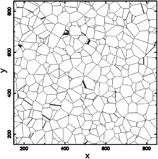
Figure 1: PVT diagram $V_{p}(2,3)$ when 789 2D cells generated by 15 000 3D seeds are considered.

The fit with the rescaled $f(x,b)$ is shown in Fig. 2 and Table 4 shows the $\chi^{2}$ of three different fitting functions.

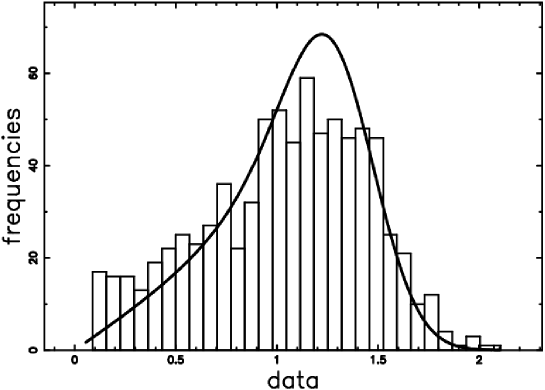
Figure 2: Histogram (step-diagram) of PVT $V_{p}(2,3)$ when 789 2D cells, generated by 15 000 3D seeds, are considered. The superposition of the $f(x,b)$, Eq. (0.3.1), is displayed.

Table 4: The values of $\chi^{2}$ for the cell normalized area-distribution of $V_{p}(2,3)$. The number of 2D cells is 789, the 3D seeds are 15 000 and the number of bins in the histogram is 30.

$$\begin{array}[]{lll}\hline\cr PDF\nobreak\leavevmode&parameters&\chi^{2}\\ \vskip 3.0pt plus 1.0pt minus 1.0pt\cr\hline\cr\vskip 3.0pt plus 1.0pt minus 1.0pt\cr H(x;c)(Eq.\leavevmode\nobreak\ (\ref{kiang}))&c=5.8&250.8\\ \vskip 3.0pt plus 1.0pt minus 1.0pt\cr\hline\cr f(x;d)(Eq.\leavevmode\nobreak\ (\ref{rumeni}))&d=3.53&250.8\\ \vskip 3.0pt plus 1.0pt minus 1.0pt\cr\hline\cr f(x,b)(Eq.\leavevmode\nobreak\ (\ref{FRMEIJERB}))&b=2.0514&127\\ \hline\cr\end{array}$$

The PDF $f_{A}$ of the areas of $V_{p}(2,3)$ can be obtained from $f(r)$ by means of the transformation, see Ferraro & Zaninetti (2011),

$$f_{A}(A)=f(r)\left(\left(\frac{A}{\pi}\right)^{1/2}\right)\frac{\pi^{-1/2}}{2}{A}^{-1/2},$$ (31)

that is,

$$f_{A}(A)=0.549\,\sqrt[6]{3}\sqrt[3]{10}G^{4,1}_{3,5}\left({\frac{100}{9}}\,{\frac{{A}^{3}}{\pi}}\,\Big{|}\,^{5/6,1/6,1/2}_{7/3,2/3,1/3,0,{\frac{17}{6}}}\right){\pi}^{-2/3}.$$ (32)

The already derived $f_{A}(A)$ has average value, variance, mode, skewness and kurtosis as shown in Table 5.

Table 5: Parameters of $f_{A}(A)$, Eq. (32), relative to the $PVT$ case.

$$\begin{array}[]{ll}\hline\cr Parameter\nobreak\leavevmode&value\\ \vskip 3.0pt plus 1.0pt minus 1.0pt\cr\hline\cr\vskip 3.0pt plus 1.0pt minus 1.0pt\cr Mean&0.824\\ \vskip 3.0pt plus 1.0pt minus 1.0pt\cr\hline\cr Variance&0.204\\ \vskip 3.0pt plus 1.0pt minus 1.0pt\cr\hline\cr Mode&0.858\\ \hline\cr Skewness&0.278\\ \hline\cr Kurtosis&-0.337\\ \hline\cr\end{array}$$

Since, for $r$ close to $0$, $f(r)\sim r$ from Eq. (32) it follows that $f_{A}(0)\neq 0$, in particular $f_{A}(0)=0.443$ and Fig. 3 shows the graph of $f_{A}$.

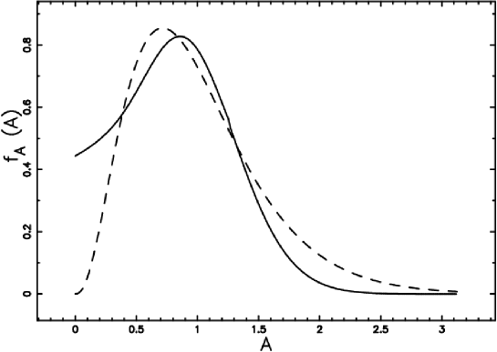
Figure 3: The PDF $f_{A}$, Eq. (32), as a function of $A$ (full line) and FN(x;d), Eq. (4), when d=2 (dotted line).

The previous figure shows that sections through 3-dimensional Voronoi tessellations are not themselves 2-dimensional Voronoi tessellations because $f_{A}(0)$ has a finite value rather than 0 as does the 2D area distribution; this fact can be considered a numerical demonstration in agreement with Chiu et al. (1996). The distribution function $F_{A}$ is given by

$$F_{A}=0.018\,{3}^{5/6}{10}^{2/3}G^{4,2}_{4,6}\left({\frac{100}{9}}\,{\frac{{A}^{3}}{\pi}}\,\Big{|}\,^{1,7/6,1/2,5/6}_{8/3,1,2/3,1/3,{\frac{19}{6}},0}\right){\frac{1}{\sqrt[3]{\pi}}}.$$ (33)

Consider a three-dimensional Poisson Voronoi diagram and suppose it intersects a randomly oriented plane $\gamma$: the resulting cross sections are polygons.

A comparison between $F_{A}$ and the area of the irregular polygons is shown in Fig. 4. In this case the number of seeds is $300000$ and we processed $100168$ irregular polygons obtained by adding together results of cuts by $41$ triples of mutually perpendicular planes. The maximum distance between the two curves is $d_{max}=0.039$.

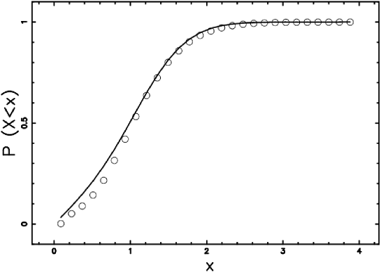
Figure 4: Comparison between data (empty circles) and theoretical curve (continuous line) of the distribution of areas of the planar cross sections.

As concerns the linear dimension, in our approximation the two-dimensional cells were considered circles and thus, for consistency, the radius $r$ of an irregular polygon was defined as

$$r=\left(\frac{A}{\pi}\right)^{1/2},$$ (34)

that is, $r$ is the radius of a circle with the same area, $A$, as the polygon. The assumption of sphericity can be considered an axiom of the theory here presented, but for a more realistic situation the stereological results will be far more complex.

0.4 Statistics of the voids

This section first processes 1024 observed cosmic voids and then derives the same results from the stereological point of view.

0.4.1 Observed statistics

The distribution of the effective radius and the radius of the maximal enclosed sphere between galaxies of the Sloan Digital Sky Survey Data Release 7 (SDSS DR7) has been reported in Pan et al. (2011). This catalog contains 1054 voids: Table 6 shows the basic statistical parameters of the effective radius, and Table 7, the radius of the maximal enclosed sphere.

Table 6: The statistical parameters of the effective radius in SDSS DR7.

$$\begin{array}[]{lc}\hline\cr\hline\cr\vskip 3.0pt plus 1.0pt minus 1.0pt\cr parameter&value\\ \vskip 3.0pt plus 1.0pt minus 1.0pt\cr elements&1024\\ \vskip 3.0pt plus 1.0pt minus 1.0pt\cr mean&18.23h^{-1}\leavevmode\nobreak\ Mpc\\ \vskip 3.0pt plus 1.0pt minus 1.0pt\cr variance&23.32h^{-2}\leavevmode\nobreak\ Mpc^{2}\\ \vskip 3.0pt plus 1.0pt minus 1.0pt\cr standard\leavevmode\nobreak\ deviation&4.82h^{-1}\leavevmode\nobreak\ Mpc\\ \vskip 3.0pt plus 1.0pt minus 1.0pt\cr skewness&0.51\\ \vskip 3.0pt plus 1.0pt minus 1.0pt\cr kurtosis&0.038\\ \vskip 3.0pt plus 1.0pt minus 1.0pt\cr maximum\leavevmode\nobreak\ value&34.12h^{-1}\leavevmode\nobreak\ Mpc\\ \vskip 3.0pt plus 1.0pt minus 1.0pt\cr minimum\leavevmode\nobreak\ value&9.9h^{-1}\leavevmode\nobreak\ Mpc\\ \vskip 3.0pt plus 1.0pt minus 1.0pt\cr\hline\cr\hline\cr\end{array}$$

Table 7: The statistical parameters of the radius of the maximal enclosed sphere in SDSS DR7.

$$\begin{array}[]{lc}\hline\cr\hline\cr\vskip 3.0pt plus 1.0pt minus 1.0pt\cr parameter&value\\ \vskip 3.0pt plus 1.0pt minus 1.0pt\cr elements&1054\\ \vskip 3.0pt plus 1.0pt minus 1.0pt\cr mean&12.95h^{-1}\leavevmode\nobreak\ Mpc\\ \vskip 3.0pt plus 1.0pt minus 1.0pt\cr variance&6.99^{-2}\leavevmode\nobreak\ Mpc^{2}\\ \vskip 3.0pt plus 1.0pt minus 1.0pt\cr standard\leavevmode\nobreak\ deviation&2.64h^{-1}\leavevmode\nobreak\ Mpc\\ \vskip 3.0pt plus 1.0pt minus 1.0pt\cr skewness&1.47\\ \vskip 3.0pt plus 1.0pt minus 1.0pt\cr kurtosis&2.401\\ \vskip 3.0pt plus 1.0pt minus 1.0pt\cr maximum\leavevmode\nobreak\ value&25.69h^{-1}\leavevmode\nobreak\ Mpc\\ \vskip 3.0pt plus 1.0pt minus 1.0pt\cr minimum\leavevmode\nobreak\ value&10h^{-1}\leavevmode\nobreak\ Mpc\\ \vskip 3.0pt plus 1.0pt minus 1.0pt\cr\hline\cr\hline\cr\end{array}$$

0.4.2 PVT statistics

Fig. 5 shows a superposition of the effective radius of the voids in the SDSS DR7 with a the curve of the theoretical PDF in the radii, $F(R,b)$, as given by Eq. (21). Table 8 shows the theoretical statistical parameters.

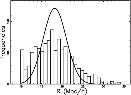
Figure 5: Histogram (step-diagram) of the effective radius in SDSS DR7 with a superposition of the PDF in radius of the PVT spheres, $F(R,b)$, as represented by Eq. (21). The number of bins is 30, and b = 30.05 Mpc.

Table 8: The statistical parameters of the theoretical radius of the PVT spheres as represented by Eq. (21) when b=30.05 Mpc.

$$\begin{array}[]{lc}\hline\cr\hline\cr\vskip 3.0pt plus 1.0pt minus 1.0pt\cr parameter&value\\ \vskip 3.0pt plus 1.0pt minus 1.0pt\cr mean&18.23h^{-1}\leavevmode\nobreak\ Mpc\\ \vskip 3.0pt plus 1.0pt minus 1.0pt\cr variance&7.70h^{-2}\leavevmode\nobreak\ Mpc^{2}\\ \vskip 3.0pt plus 1.0pt minus 1.0pt\cr standard\leavevmode\nobreak\ deviation&2.77h^{-1}\leavevmode\nobreak\ Mpc\\ \vskip 3.0pt plus 1.0pt minus 1.0pt\cr mode&18.49h^{-1}\leavevmode\nobreak\ Mpc\\ \vskip 3.0pt plus 1.0pt minus 1.0pt\cr skewness&0.0142\\ \vskip 3.0pt plus 1.0pt minus 1.0pt\cr kurtosis&-0.0514\\ \vskip 3.0pt plus 1.0pt minus 1.0pt\cr\hline\cr\end{array}$$

Table 9 shows the values of $\chi^{2}$ for the main PDFs here considered.

Table 9: Values of $\chi^{2}$ for the effective radius in SDSS DR7 for different distributions when the number of bins is 30. In this comparison, the averaged value of the astronomical radii is one.

$$\begin{array}[]{lll}\hline\cr PDF\nobreak\leavevmode&parameters&\chi^{2}\\ \vskip 3.0pt plus 1.0pt minus 1.0pt\cr\hline\cr\vskip 3.0pt plus 1.0pt minus 1.0pt\cr H(x;c),(Eq.(\ref{kiang}))&c=14.24&53\\ \vskip 3.0pt plus 1.0pt minus 1.0pt\cr\hline\cr f(x;d),(Eq.(\ref{rumeni}))&d=9.1&53\\ \vskip 3.0pt plus 1.0pt minus 1.0pt\cr\hline\cr f(x,b),(Eq.(\ref{FRMEIJERB}))&b=2.051&182\\ \hline\cr F(R,b),(Eq.(\ref{RUMENIRB}))&b=1.648&407\\ \hline\cr F_{K}(R,b,c),(Eq.(\ref{KIANGVARC})&b=31.33\leavevmode\nobreak\ c=1.76&66.121\\ \hline\cr\end{array}$$

The statistics of the voids can also be visualized through the SF, see an application to the 2dFGRS as given by Patiri et al. (2006); von Benda-Beckmann & Müller (2008).

The statistics of the voids between galaxies have been also analysed in von Benda-Beckmann & Müller (2008) with the following self-similar SF in the following, $S_{SS}$,

$$S_{SS}={{\rm e}^{-\left({\frac{R}{s_{{1}}\lambda}}\right)^{p_{{1}}}-\left({\frac{R}{s_{{2}}\lambda}}\right)^{p_{{2}}}}},$$ (35)

where $\lambda$ is the mean separation between galaxies, $s_{1}$ and $s_{2}$ are two length factors, and $p_{1}$ and $p_{2}$ two powers. A final comparison between the four samples of void size statistics as represented in Fig. 4 of von Benda-Beckmann & Müller (2008) and our survival function of the radius for $V_{p}(2,3)$ as given by Eq. (0.3.1) is shown in Fig. 6.

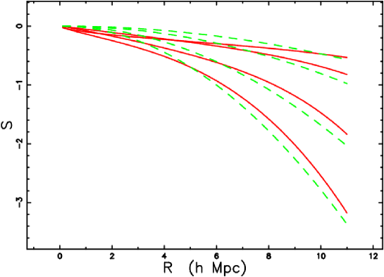
Figure 6: The survival function, $S_{SS}$, for the self-similar distribution in radius of $N/S1$, $N/S2$, $N/S3$ and $N/S4$, as reported in Fig. 4 of von Benda-Beckmann & Müller (2008) (full red lines), as represented by (35). The survival function, $SF(x,b)$, of the radius of the distribution which involves the Meijer $G$-function for $V_{p}(2,3)$ as represented by (0.3.1) when $b=12$ Mpc, $b=14$ Mpc, $b=17$ Mpc, and $b=19$ Mpc (dashed green lines).

More details as well the PDF of the self-similar distribution can be found in Zaninetti (2010).

0.5 NPVT statistics

An example of non NPVT is represented by a distribution in volume which follows a Kiang function as given by Eq. (1). The case of PVT volumes indicates $c=5$, see Eq. (8), or $c=6$, the so called Kiang conjecture: we will take $c$ as a variable. The resulting distribution in radius once the scaling parameter $b$ is introduced is

$$F_{K}(R,b,c)=\frac{4\,c\left(4/3\,{\frac{c\pi\,{R}^{3}}{{b}^{3}}}\right)^{c-1}{{\rm e}^{-4/3\,{\frac{c\pi\,{R}^{3}}{{b}^{3}}}}}\pi\,{R}^{2}}{\Gamma\left(c\right){b}^{3}}.$$ (36)

The average radius is

$$\overline{R}=\frac{\sqrt[3]{2}\sqrt[3]{3}b\Gamma\left(1/3+c\right)}{2\,\sqrt[3]{c}\sqrt[3]{\pi}\Gamma\left(c\right)},$$ (37)

and the variance is

$$\sigma^{2}(R)=\frac{-{3}^{2/3}{2}^{2/3}{b}^{2}\left(-\Gamma\left(2/3+c\right)\Gamma\left(c\right)+\left(\Gamma\left(1/3+c\right)\right)^{2}\right)}{4\,{c}^{2/3}{\pi}^{2/3}\left(\Gamma\left(c\right)\right)^{2}}.$$ (38)

The skewness is

$$\gamma=\frac{\left(\Gamma\left(c\right)\right)^{3}c-3\,\Gamma\left(c\right)\Gamma\left(1/3+c\right)\Gamma\left(2/3+c\right)+2\,\left(\Gamma\left(1/3+c\right)\right)^{3}}{\left(\Gamma\left(2/3+c\right)\Gamma\left(c\right)-\left(\Gamma\left(1/3+c\right)\right)^{2}\right)^{3/2}},$$ (39)

and the kurtosis is given by a complicated analytical expression. Fig. 7 shows a superposition of the effective radii of the voids in SDSS DR7 with a superposition of the curve of the theoretical PDF in the radius, $F_{K}(R,b,c)$, as represented by Eq. (36). Table 9 shows the values of $\chi^{2}$ . Table 10 shows the theoretical statistical parameters.

Figure 7: Histogram (step-diagram) of the effective radius in the SDSS DR7 with a superposition of the PDF in radius of the NPVT spheres, $F_{K}(R,b,c)$, as represented by Eq. (36). The number of bins is 30, $b$=31.33 Mpc, and $c=1.768$.

Table 10: The statistical parameters of the theoretical radius of the NPVT spheres as represented by Eq. (36) when ${b}$=31.33 Mpc and ${c}=1.768$.

$$\begin{array}[]{lc}\hline\cr\hline\cr\vskip 3.0pt plus 1.0pt minus 1.0pt\cr parameter&value\\ \vskip 3.0pt plus 1.0pt minus 1.0pt\cr mean&18.23h^{-1}\leavevmode\nobreak\ Mpc\\ \vskip 3.0pt plus 1.0pt minus 1.0pt\cr variance&23.31h^{-2}\leavevmode\nobreak\ Mpc^{2}\\ \vskip 3.0pt plus 1.0pt minus 1.0pt\cr standard\leavevmode\nobreak\ deviation&4.82h^{-1}\leavevmode\nobreak\ Mpc\\ \vskip 3.0pt plus 1.0pt minus 1.0pt\cr skewness&0.072\\ \vskip 3.0pt plus 1.0pt minus 1.0pt\cr kurtosis&-0.162\\ \vskip 3.0pt plus 1.0pt minus 1.0pt\cr\hline\cr\end{array}$$

The result of the integration of the fundamental Eq. (11) inserting $c$=2 gives the following PDF for the radius of the cuts

$$f(r)_{NPVTK}=3.4148\,\sqrt[6]{3}\sqrt[3]{\pi}r{2}^{2/3}G^{4,0}_{2,4}\left({\frac{16}{9}}\,{\pi}^{2}{r}^{6}\,\Big{|}\,^{1/6,1/2}_{4/3,2/3,1/3,0}\right)$$ (40)

$$\quad 0\leq r\leq 1.$$

The statistics of NPVT cuts with $c$=2 are shown in Table 11.

Table 11: NPVT parameters of $f(r)_{NPVTK}$, Eq. (0.5).

$$\begin{array}[]{ll}\hline\cr Parameter\nobreak\leavevmode&value\\ \vskip 3.0pt plus 1.0pt minus 1.0pt\cr\hline\cr\vskip 3.0pt plus 1.0pt minus 1.0pt\cr Mean&0.488\\ \vskip 3.0pt plus 1.0pt minus 1.0pt\cr\hline\cr Variance&0.0323\\ \vskip 3.0pt plus 1.0pt minus 1.0pt\cr\hline\cr Mode&0.517\\ \hline\cr Skewness&-.114\\ \hline\cr Kurtosis&2.614\\ \hline\cr\end{array}$$

On introducing the scaling parameter $b$, the PDF which describes the radius of the cut becomes

$$f(x,b)_{NPVTK}=3.4148\,\sqrt[6]{3}\sqrt[3]{\pi}x{2}^{2/3}G^{4,0}_{2,4}\left({\frac{16}{9}}\,{\frac{{\pi}^{2}{x}^{6}}{{b}^{6}}}\,\Big{|}\,^{1/6,1/2}_{4/3,2/3,1/3,0}\right){b}^{-2}$$ (41)

$$\quad 0\leq r\leq b.$$

The SF of the second NPVT case, $SF_{NPVTK}$, with the scaling parameter $b$, is

$$SF(x,b)_{NPVTK}=1-0.2845\,{3}^{5/6}\sqrt[3]{2}G^{4,1}_{3,5}\left({\frac{16}{9}}\,{\frac{{\pi}^{2}{x}^{6}}{{b}^{6}}}\,\Big{|}\,^{1,1/2,5/6}_{5/3,1,2/3,1/3,0}\right){\frac{1}{\sqrt[3]{\pi}}}$$ (42)

$$\quad 0\leq r\leq b.$$

A careful exploration of the distribution in effective radius of SDSS DR7 reveals that the detected voids have radius $\geq$ 10/h Mpc. This observational fact demands the generation of random numbers in the distribution in radii of the 3D cells as given by Eq. (36) with a minimal value of 10/h Mpc. The artificial sample is generated through a numerical computation of the inverse function Brandt & Gowan (1998) and displayed in Fig. 8; the sample’s statistics are shown in Table 12.

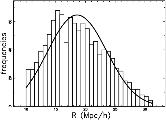
Figure 8: Histogram (step-diagram) of the simulated effective radius of SDSS DR7 with a superposition of the PDF in radius of the PVT spheres as represented by Eq. (36). The artificial sample has a minimum value of 10/h Mpc, the number of bins is 30, $b$= 31.5/h Mpc, and $c=1.3$.

Table 12: The statistical parameters of the artificially generated radius with a lower bound of 10 /h Mpc, $c=1.3$ and $b$ =31.5/h Mpc.

$$\begin{array}[]{lc}\hline\cr\hline\cr\vskip 3.0pt plus 1.0pt minus 1.0pt\cr parameter&value\\ \vskip 3.0pt plus 1.0pt minus 1.0pt\cr mean&18.69h^{-1}\leavevmode\nobreak\ Mpc\\ \vskip 3.0pt plus 1.0pt minus 1.0pt\cr variance&22.74h^{-2}\leavevmode\nobreak\ Mpc^{2}\\ \vskip 3.0pt plus 1.0pt minus 1.0pt\cr standard\leavevmode\nobreak\ deviation&4.76h^{-1}\leavevmode\nobreak\ Mpc\\ \vskip 3.0pt plus 1.0pt minus 1.0pt\cr skewness&0.33\\ \vskip 3.0pt plus 1.0pt minus 1.0pt\cr kurtosis&-0.623\\ \vskip 3.0pt plus 1.0pt minus 1.0pt\cr maximum\leavevmode\nobreak\ value&31.27h^{-1}\leavevmode\nobreak\ Mpc\\ \vskip 3.0pt plus 1.0pt minus 1.0pt\cr minimum\leavevmode\nobreak\ value&10h^{-1}\leavevmode\nobreak\ Mpc\\ \vskip 3.0pt plus 1.0pt minus 1.0pt\cr\hline\cr\hline\cr\end{array}$$

0.6 Conclusions

PVT Statistics The approach as given by the stereology to the PDF in radii of the circles which result from the intersection between a plane and a randomly disposed spheres of radius $R$ is actually limited to the case of mono-disperse spheres of radius $R$ and to a power law with radius $\propto R^{-\alpha}$ Blower et al. (2002). Here adopting the same type of demonstration we simply substitute into formula (11) a new distribution for the generalized radii, $(R)$, of PVT. The resulting distribution in radii, $(r)$, of the circles of intersection involves the Meijer $G$-function. A first test on this new PDF for the radii was performed on the 2dFGRS catalog and the theoretical $V_{p}(2,3)$ cells were compared with other fitting functions, see Fig. 6.

NPVT Statistics

Among the infinite number of 3D seeds which are non-Poissonian, we selected a distribution in volume which follows a Kiang function as given by Eq. (1) with $c\approx$2.

A careful comparison with the measured effective radii permits us to say that the NPVT case here considered is a good model because it can reproduce the 3D average radius and the variance, see Table 10. The model for the effective radius of the voids as given by the Kiang distribution in volumes with $c$ variable can also be used to generate an artificial sample of the effective radius of the voids, see Fig. 8 and Table 12.

.7 The Meijer $G$-function

In general the Meijer $G$-function is defined by the following Mellin–Barnes type integral on the complex plane,

$${cc}G_{p,q}^{m,n}(z) \equiv G_{p,q}^{m,n}\left(z\left|\begin{array}[]{c}(a_{i})_{1}^{p}\\ \\ (b_{j})_{1}^{q}\end{array}\right.\right)\equiv G_{p,q}^{m,n}\left(z\left|\begin{array}[]{cc}a_{1},\dots,a_{p}\\ \\ b_{1},\dots,b_{q}\end{array}\right.\right)$$ (49)

$$= \displaystyle\frac{1}{2\pi i}\displaystyle\int_{\mathcal{L}}\frac{\displaystyle\prod_{j=1}^{m}\Gamma(b_{j}+s)\prod_{j=1}^{n}\Gamma(1-a_{j}-s)}{\displaystyle\prod_{j=n+1}^{p}\Gamma(a_{j}+s)\prod_{j=m+1}^{q}\Gamma(1-b_{j}-s)}z^{-s}ds,$$ (50)

where the contour of integration $\mathcal{L}$ is arranged to lie between the poles of $\Gamma(a_{i}+s)$ and the poles of $\Gamma(b_{j}+s)$. The $G$-function is defined under the following hypothesis.

• $0\leq m\leq q,0\leq n\leq p$, and $p\leq q-1$;

• $z\neq 0$;

• no pair of $b_{j}$, $j$ distinct, $j=1,2,\dots,m$ differ by an integer or zero;

• the parameters $a_{i}\in\mathrm{C}$ and $b_{j}\in\mathrm{C}$ are such that no pole of $\Gamma(b_{j}+s),j=1,2,\dots,m$ coincide with any pole of $\Gamma(a_{i}+s),i=1,2,\dots,n$;

• $a_{i}-b_{j}\neq 1,2,3,\dots$ for $i=1,2,\dots,n$ and $j=1,2,\dots,m$; and

• if $p=q$, then the definition makes sense only for $|z|<1$, see Meijer (1936, 1941); Ho et al. (2007); Olver et al. (2010).

References

- Abazajian et al. (2009) Abazajian, K. N., Adelman-McCarthy, J. K., Agüeros, M. A., Allam, S. S., Allende Prieto, C., & et al. 2009, ApJS , 182, 543
- Barrow & Coles (1990) Barrow, J. D. & Coles, P. 1990, MNRAS , 244, 188
- Bernardeau & van de Weygaert (1996) Bernardeau, F. & van de Weygaert, R. 1996, MNRAS , 279, 693
- Blower et al. (2002) Blower, J., Keating, J., Mader, H., & Phillips, J. 2002, Journal of Volcanology and Geothermal Research, 120, 1
- Brandt & Gowan (1998) Brandt, S. & Gowan, G. 1998, Data Analysis: Statistical and Computational Methods for Scientists and Engineers (New York: Springer-Verlag).
- Bratley, P. and Fox, B. L. (1988) Bratley, P. and Fox, B. L. 1988, ACM Trans. Math. Softw., 14, 88
- Chiu et al. (1996) Chiu, S. N., Weygaert, R. V. D., & Stoyan, D. 1996, Adv. in Appl. Prob., 28, 356
- Coles (1991) Coles, P. 1991, Nature , 349, 288
- Colless et al. (2001) Colless, M., Dalton, G., Maddox, S., & et al. 2001, MNRAS , 328, 1039
- Ebeling & Wiedenmann (1993) Ebeling, H. & Wiedenmann, G. 1993, Phys. Rev. E , 47, 704
- Elyiv et al. (2009) Elyiv, A., Melnyk, O., & Vavilova, I. 2009, MNRAS , 394, 1409
- Ferenc & Néda (2007) Ferenc, J.-S. & Néda, Z. 2007, Phys. A , 385, 518
- Ferraro & Zaninetti (2011) Ferraro, M. & Zaninetti, L. 2011, Phys. Rev. E , 84, 041107
- Geller & Huchra (1989) Geller, M. J. & Huchra, J. P. 1989, Science, 246, 897
- Goldwirth et al. (1995) Goldwirth, D. S., da Costa, L. N., & van de Weygaert, R. 1995, MNRAS , 275, 1185
- Ho et al. (2007) Ho, M.-W., James, L. F., & Lau, J. W. 2007, ArXiv e-prints
- Icke & van de Weygaert (1987) Icke, V. & van de Weygaert , R. 1987, A&A , 184, 16
- Ikeuchi & Turner (1991) Ikeuchi, S. & Turner, E. L. 1991, MNRAS , 250, 519
- Kiang (1966) Kiang, T. 1966, Z. Astrophys. , 64, 433
- Marinoni et al. (2002) Marinoni, C., Davis, M., Newman, J. A., & Coil, A. L. 2002, ApJ , 580, 122
- Meijer (1936) Meijer, C. 1936, Nieuw Arch. Wiskd., 18, 10
- Meijer (1941) —. 1941, Proc. Akad. Wet. Amsterdam, 44, 1062
- Melnyk et al. (2006) Melnyk, O. V., Elyiv, A. A., & Vavilova, I. B. 2006, Kinematika i Fizika Nebesnykh Tel, 22, 283
- Møller (1989) Møller, J. 1989, Adv. Appl. Probab., 21, 37
- Møller (1994) —. 1994, Lectures on Random Voronoi Tessellations. (Lecture Notes in Statistics. 87) (New York: Springer-Verlag).
- Okabe et al. (1992) Okabe, A., Boots, B., & Sugihara, K. 1992, Spatial tessellations. Concepts and Applications of Voronoi diagrams (Chichester, NY: Wiley)
- Olver et al. (2010) Olver, F., Lozier, D., Boisvert, R., & Clark, C. 2010, NIST Handbook of Mathematical Functions. (Cambridge: Cambridge University Press.)
- Pan et al. (2011) Pan, D. C., Vogeley, M. S., Hoyle, F., Choi, Y.-Y., & Park, C. 2011, ArXiv e-prints:1103.4156
- Patiri et al. (2006) Patiri, S. G., Betancort-Rijo, J. E., Prada, F., Klypin, A., & Gottlöber, S. 2006, MNRAS , 369, 335
- Pierre (1990) Pierre, M. 1990, A&A , 229, 7
- Press et al. (1992) Press, W. H., Teukolsky, S. A., Vetterling, W. T., & Flannery, B. P. 1992, Numerical Recipes in FORTRAN. The Art of Scientific Computing (Cambridge: Cambridge University Press)
- Schaap & van de Weygaert (2000) Schaap, W. E. & van de Weygaert, R. 2000, A&A , 363, L29
- Sobol, I.M. (1967) Sobol, I.M. 1967, U.S.S.R. Comput. Math. Math. Phys., 7, 86
- Subba Rao & Szalay (1992) Subba Rao, M. U. & Szalay, A. S. 1992, ApJ , 391, 483
- van de Weygaert (1991) van de Weygaert , R. 1991, MNRAS , 249, 159
- van de Weygaert (1991) van de Weygaert, R. 1991, Ph.D. thesis, University of Leiden
- van de Weygaert (1994) —. 1994, A&A , 283, 361
- van de Weygaert (2002) —. 2002, arXiv:astro-ph/0206427
- van de Weygaert (2003) —. 2003, Statistics of Galaxy Clustering - Commentary (Statistical Challenges in Astronomy), 156–186
- van de Weygaert & Icke (1989) van de Weygaert, R. & Icke, V. 1989, A&A , 213, 1
- van de Weygaert & Schaap (2009) van de Weygaert, R. & Schaap, W. 2009, in V. J. Martinez, E. Saar, E. M. Gonzales, & M. J. Pons-Borderia, eds, Lecture Notes in Physics Vol. 665 (Berlin: Springer-Verlag), pp. 291–311.
- von Benda-Beckmann & Müller (2008) von Benda-Beckmann, A. M. & Müller, V. 2008, MNRAS , 384, 1189
- Voronoi (1907) Voronoi, G. 1907, J. Reine Angew. Math., 133, 97
- Voronoi (1908) —. 1908, J. Reine Angew. Math., 134, 198
- York et al. (2000) York, D. G., Adelman, J., Anderson Jr., J. E., Anderson, S. F., Annis, J., Bahcall, N. A., Bakken, J. A., & et al. 2000, AJ , 120, 1579
- Zaninetti (1991) Zaninetti, L. 1991, A&A , 246, 291
- Zaninetti (2006) —. 2006, Chinese J. Astron. Astrophys. , 6, 387
- Zaninetti (2010) —. 2010, Serbian Astr. Jour., 181, 19