Hyperon vector form factor from 2+1 flavor lattice QCD

Abstract

We present the first result for the hyperon vector form factor $f_{1}$ for $\Xi^{0}\rightarrow\Sigma^{+}l\bar{\nu}$ and $\Sigma^{-}\rightarrow nl\bar{\nu}$ semileptonic decays from fully dynamical lattice QCD. The calculations are carried out with gauge configurations generated by the RBC and UKQCD collaborations with (2+1)-flavors of dynamical domain-wall fermions and the Iwasaki gauge action at $\beta=2.13$, corresponding to a cutoff $a^{-1}=1.73$ GeV. Our results, which are calculated at the lighter three sea quark masses (the lightest pion mass down to approximately 330 MeV), show that a sign of the second-order correction of SU(3) breaking on the hyperon vector coupling $f_{1}(0)$ is negative. The tendency of the SU(3) breaking correction observed in this work disagrees with predictions of both the latest baryon chiral perturbation theory result and large $N_{c}$ analysis.

I Introduction

Greater knowledge of the vector form factor $f_{1}$ in $\Delta S=1$ semileptonic hyperon decays paves the way for an alternative determination of the element $V_{us}$ of the Cabibbo-Kobayashi-Maskawa (CKM) matrix in addition to kaon semileptonic ($K_{l3}$) decays, leptonic decays of kaons and pions, and hadronic decays of $\tau$ leptons . A stringent test of CKM unitarity through the first row relation $|V_{ud}|^{2}+|V_{us}|^{2}+|V_{ub}|^{2}=1$ can be accomplished with the precision of $|V_{us}|$ BM . A theoretical estimation of the vector coupling $f_{1}(0)$ is required to extract $V_{us}$ from the experimental rate of hyperon beta decay Cabibbo:2003cu ; Mateu:2005wi .

The matrix element for hyperon beta decays, $B_{1}\rightarrow B_{2}l\bar{\nu}$, is composed of the vector and axial-vector transitions, $\langle B_{2}(p^{\prime})|V_{\alpha}(x)+A_{\alpha}(x)|B_{1}(p)\rangle$, which are described by six form factors: the vector ($f_{1}$), weak magnetism $(f_{2})$, and induced scalar $(f_{3})$ form factors for the vector current, and the axial-vector $(g_{1})$, weak electricity $(g_{2})$, and induced pseudo-scalar $(g_{3})$ form factors for the axial current Cabibbo:2003cu . The experimental decay rate of the hyperon beta decay, $B_{1}\rightarrow B_{2}$, is given by

$$\Gamma = \frac{G_{F}^{2}}{60\pi^{3}}(M_{B_{1}}-M_{B_{2}})^{5}(1-3\delta)|V_{us}|^{2}|f^{B_{1}\rightarrow B_{2}}_{1}(0)|^{2}$$ (2)

$$\times(1+\Delta_{\rm RC})\left[1+3\left|\frac{g^{B_{1}\rightarrow B_{2}}_{1}(0)}{f^{B_{1}\rightarrow B_{2}}_{1}(0)}\right|^{2}+\cdot\cdot\cdot\right],$$

where $G_{F}$ is the Fermi constant measured from the muon life time, which already includes some electroweak radiative corrections Cabibbo:2003cu . The remaining radiative corrections to the decay rate are approximately represented by $\Delta_{\rm RC}$ Garcia:1985xz . Here, $M_{B_{1}}$ ($M_{B_{2}}$) denotes the rest mass of the initial (final) octet baryon state. The ellipsis can be expressed in terms of a power series in the small parameter $\delta=(M_{B_{1}}-M_{B_{2}})/(M_{B_{1}}+M_{B_{2}})$, which is regarded as a size of flavor SU(3) breaking Gaillard:1984ny . The first linear term in $\delta$, which should be given by $-4\delta[g_{2}(0)g_{1}(0)/f_{1}(0)^{2}]_{B_{1}\rightarrow B_{2}}$ , is safely ignored as small as ${\cal O}(\delta^{2})$ since the nonzero value of the second-class form factor $g_{2}$ Weinberg:1958ut should be induced at first order of the $\delta$ expansion Gaillard:1984ny . The absolute value of $g_{1}(0)/f_{1}(0)$ can be determined by measured asymmetries such as electron-neutrino correlation Cabibbo:2003cu ; Gaillard:1984ny . A theoretical attempt to evaluate SU(3)-breaking corrections on the vector coupling $f_{1}(0)$, whose value is given by SU(3) Clebsch-Gordan coefficients in the exact SU(3) limit, is primarily required for the precise determination of $|V_{us}|$.

The value of $f_{1}(0)$ should be equal to the SU(3) Clebsch-Gordan coefficients up to the second order in SU(3) breaking, thanks to the Ademollo-Gatto theorem (AGT) Ademollo:1964sr . As the mass splittings among octet baryons are typically of the order of 10-15%, an expected size of the second-order corrections is a few percent level. However, either the size or the sign of their corrections is somewhat controversial among various theoretical studies at present as summarized in Table 1. A model independent evaluation of SU(3)-breaking corrections is highly desired. Although recent quenched lattice studies suggest that the second-order correction on $f_{1}(0)$ is likely negative Guadagnoli:2006gj ; Sasaki:2008ha , we need further confirmation from (2+1)-flavor dynamical lattice QCD near the physical point.

Our paper is organized as follows. In Sec. II, we first summarize the numerical lattice QCD ensembles used for this work and then give the details of our Monte Carlo simulations. The numerical results are presented in Sec. III. We begin with our determination of the scalar form factor $f_{S}(q^{2})$, which will be defined in the later session, at finite momentum transfer. We discuss in detail the interpolation of the form factor to zero momentum transfer and also the chiral extrapolation of the hyperon vector coupling $f_{1}(0)$. Finally, in Sec. VI, we summarize our results and conclusions.

Table 1: Theoretical uncertainties of $\tilde{f}_{1}(0)=f_{1}(0)/f_{1}^{\rm SU(3)}(0)$ for various hyperon beta-decays. HBChPT and EOMS-CBChPT stand for heavy baryon chiral perturbation theory and covariant baryon chiral perturbation theory with the extended on-mass-shell (EOMS) renormalization scheme.

Type of result (reference)	$\Lambda\rightarrow p$	$\Sigma^{-}\rightarrow n$	$\Xi^{-}\rightarrow\Lambda$	$\Xi^{0}\rightarrow\Sigma^{+}$
Bag model Donoghue:1981uk	0.97	0.97	0.97	0.97
Quark model  Donoghue:1986th	0.987	0.987	0.987	0.987
Quark model Schlumpf:1994fb	0.976	0.975	0.976	0.976
$1/N_{c}$ expansion Flores-Mendieta:1998ii	1.02(2)	1.04(2)	1.10(4)	1.12(5)
Full ${\cal O}(p^{4})$ HBChPT Villadoro:2006nj	1.027	1.041	1.043	1.009
Full ${\cal O}(p^{4})$ + partial ${\cal O}(p^{5})$ HBChPT Lacour:2007wm	1.066(32)	1.064(6)	1.053(22)	1.044(26)
Full ${\cal O}(p^{4})$ EOMS-CBChPT Geng:2009ik	0.943(21)	1.028(02)	0.989(17)	0.944(16)
Full ${\cal O}(p^{4})$ EOMS-CBChPT + Decuplet Geng:2009ik	1.001(13)	1.087(42)	1.040(28)	1.017(22)
Quenched lattice QCD Guadagnoli:2006gj ; Sasaki:2008ha	N/A	0.988(29)	N/A	0.987(19)

II Simulation details

In this paper, we will present the first result for the hyperon vector form factor for $\Xi^{0}\rightarrow\Sigma^{+}l\bar{\nu}$ and $\Sigma^{-}\rightarrow nl\bar{\nu}$ semileptonic decays from simulations with 2+1 flavors of domain wall fermions (DWFs). We use the RBC and UKQCD collaboration ensembles, which are generated on a $24^{3}\times 64$ lattice with two light degenerate quarks and a single flavor heavier quark and the Iwasaki gauge action at $\beta=2.13$ Allton:2008pn . The dynamical light and strange quarks are described by DWF actions with fifth dimensional extent $L_{s}=16$ and the domain-wall height of $M_{5}=1.8$, which give a residual mass of $am_{\rm res}\approx 0.003$. Each ensemble of configurations uses the same dynamical strange quark mass, $am_{s}=0.04$, which is close to its physical value Allton:2008pn . We have already published our findings in nucleon structure from the same ensembles in three publications, Refs. Yamazaki:2008py ; Yamazaki:2009zq ; Aoki:2010xg .

The inverse of lattice spacing is $a^{-1}=1.73(3)$ [$a$=0.114(2) fm], which is determined from the $\Omega^{-}$ baryon mass Allton:2008pn . Accordingly, the physical spatial extent is approximately 2.7 fm, where the nucleon vector form factor at low $q^{2}$ doesn’t suffer much from the finite size effect though such effect may influence other nucleon form factors Yamazaki:2008py ; Yamazaki:2009zq . We choose three values for the light quark masses, $am_{ud}=0.005$, 0.01, and 0.02, which correspond to about 330 MeV, 420 MeV and 560 MeV pion masses . We use 4780, 2350, and 1580 trajectories separated by 20 trajectories for $am_{ud}=0.005$, 0.01, and 0.02 Allton:2008pn . The total number of configurations is 240 for $am_{ud}=0.005$, 120 for $am_{ud}=0.01$, and 80 for $am_{ud}=0.02$ as summarized in Table 2.

We make four (two) measurements on each configuration using a single source location, which is located at $(x,y,z,t)=(6n,6n,6n,16n)$ with $n=0,1,2,3$ ($n=0,2$) for $am_{ud}=0.02$ ($am_{ud}=0.01$ and $0.005$), and then they are averaged on each configuration in order to reduce possible autocorrelations among measurements. The statistical errors are estimated by the jackknife method on such blocked measurements. The quark propagators are calculated by gauge-invariant Gaussian smearing at the source with smearing parameters $(N,\omega)=(100,7)$. Details of our calculation of the quark propagators are described in Ref. Yamazaki:2009zq .

Table 2: $N_{\rm conf}$, $N_{\rm sep}$, and $N_{\rm meas}$ denote the number fo gauge configurations, trajectory separation between each measured configuration, and the number of measurements on each configuration, respectively. The table contains the pion, kaon, nucleon, $\Sigma$-baryon, and $\Xi$-baryon mass for each ensemble.

$m_{ud}$	$N_{\rm conf}$	$N_{\rm sep}$	$N_{\rm meas}$	$M_{\pi}$ [GeV]	$M_{K}$ [GeV]	$M_{N}$ [GeV]	$M_{\Sigma}$ [GeV]	$M_{\Xi}$ [GeV]
0.005	240	20	2	0.3297(7)	0.5759(8)	1.140(12)	1.330(9)	1.431(6)
0.01	120	20	2	0.4200(12)	0.6064(11)	1.237(13)	1.386(12)	1.465(8)
0.02	80	20	4	0.5580(11)	0.6651(11)	1.412(10)	1.501(9)	1.544(8)

III Numerical Results

III.1 Scalar form factor $f_{S}(q^{2})$ at $q^{2}=q_{\rm max}^{2}$

We focus on vector couplings $f_{1}(0)$ for two different hyperon beta-decays, $\Xi^{0}\rightarrow\Sigma^{+}l\bar{\nu}$ and $\Sigma^{-}\rightarrow nl\bar{\nu}$. These decays are simply denoted by $\Xi\rightarrow\Sigma$ and $\Sigma\rightarrow N$ hereafter. We recall that $f^{\Xi\rightarrow\Sigma}_{1}(0)=+1$ and $f^{\Sigma\rightarrow N}_{1}(0)=-1$ in the exact SU(3) limit. For convenience in numerical calculations, instead of the vector form factor $f_{1}(q^{2})$, we consider the so-called scalar form factor

$$f^{B_{1}\rightarrow B_{2}}_{S}(q^{2})=f^{B_{1}\rightarrow B_{2}}_{1}(q^{2})+\frac{q^{2}}{M_{B_{1}}^{2}-M_{B_{2}}^{2}}f^{B_{1}\rightarrow B_{2}}_{3}(q^{2}),$$ (3)

where $f_{3}$ represents the second-class form factor, which is identically zero in the exact SU(3) limit Weinberg:1958ut . The renormalized value of $f_{S}(q^{2})$ at $q_{\rm max}^{2}=-(M_{B_{1}}-M_{B_{2}})^{2}<0$  can be precisely evaluated by the double ratio method proposed in Ref. Guadagnoli:2006gj , where all relevant three-point functions are determined at zero three-momentum transfer $|{\bf q}|=0$. For the three-point functions, we use the sequential source method. We use the source-sink separation of 12 lattice units following previous works related to nucleon structure Yamazaki:2008py ; Yamazaki:2009zq ; Aoki:2010xg . Details of the construction of the three-point functions from the sequential quark propagator are described in Ref. Sasaki:2003jh .

Here we note that the absolute value of the renormalized $f_{S}(q_{\rm max}^{2})$ is exactly unity in the flavor SU(3) symmetric limit, where $f_{S}(q^{2}_{\rm max})$ becomes $f_{1}(0)$, for the hyperon decays considered here. Thus, the deviation from unity in $|f_{S}(q^{2}_{\rm max})|$ is attributed to three types of the SU(3) breaking effect: (1) the recoil correction ($q^{2}_{\rm max}\neq 0$) stemming from the mass difference of $B_{1}$ and $B_{2}$ states, (2) the presence of the second-class form factor $f_{3}(q^{2})$, and (3) the deviation from unity in the renormalized $f_{1}(0)$. Taking the limit of zero four-momentum transfer of $f_{S}(q^{2})$ can separate the third effect from the others, since the scalar form factor at $q^{2}=0$, $f_{S}(0)$, is identical to $f_{1}(0)$. Indeed, our main target is to measure the third one.

In Fig. 1, we plot the absolute value of the renormalized $f_{S}(q_{\rm max}^{2})$ as a function of the current insertion time slice. Good plateaus are observed in the middle region between the source and sink points. The lines represent the average value (solid lines) and their 1 standard deviations (dashed lines) over range of $3\leq t/a\leq 8$. The obtained values of $|f_{S}(q_{\rm max}^{2})|$, which are naturally renormalized in the double ratio method, as well as $q_{\rm max}^{2}$ values are summarized in Table 3.

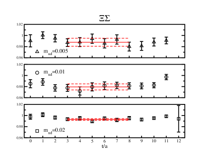
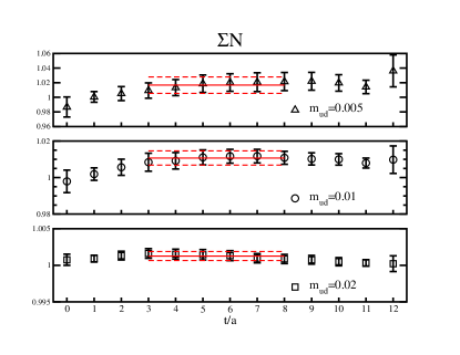
Figure 1: The absolute value of $f_{S}^{\rm ren}(q_{\rm max}^{2})$ as a function of the current insertion time slice. The upper (lower) panel is for $\Xi\rightarrow\Sigma$ ($\Sigma\rightarrow N$) decay. In each panel, results for $am_{ud}=0.005$, 0.01, and 0.02 are plotted from top to bottom. The lines represent the average value (solid lines) and their 1 standard deviations (dashed lines) over range of $3\leq t/a\leq 8$.

III.2 Interpolation to zero four-momentum squared

The scalar form factor $f_{S}(q^{2})$ at $q^{2}>0$ is also calculable with nonzero three-momentum transfer ($|{\bf q}|\neq 0$). To avoid unnecessary repetition, we simply give a reference Sasaki:2008ha , where all the technical details are available.

We use the four lowest nonzero momenta: ${\bf q}=2\pi/L\times(1,0,0)$, $(1,1,0)$, $(1,1,1)$, and $(2,0,0)$, corresponding to a $q^{2}$ range from about 0.2 to 0.8 GeV². We then can make the $q^{2}$ interpolation of $f_{S}(q^{2})$ to $q^{2}=0$ by the values of $f_{S}(q^{2})$ at $q^{2}>0$ together with the precisely measured value of $f_{S}(q^{2})$ at $q^{2}=q^{2}_{\rm max}<0$ from the double ratio.

In Fig. 2, we plot the absolute value of the renormalized $f_{S}(q^{2})$ as a function of $q^{2}$ for $\Xi\rightarrow\Sigma$ (upper panels) and $\Sigma\rightarrow N$ (lower panels) at $am_{ud}=0.005$ (left), 0.01 (middle) and 0.02 (right). In this work, we also calculate the time-reversal process $B_{2}\rightarrow B_{1}$ as well as $B_{1}\rightarrow B_{2}$, to get more data points in the $q^{2}>0$ region. Open circles are $|f_{S}(q^{2})|$ at the simulated $q^{2}$. The solid (dashed) curve is the fitting result with the seven lowest-$q^{2}$ data points by using the monopole (quadratic) interpolation form Sasaki:2008ha , while the open diamond (square) represents the interpolated value to $q^{2}=0$.

As shown in Fig. 2, two determinations to evaluate $f_{S}(0)=f_{1}(0)$ from measured points are indeed consistent with each other. Thus, this observation indicates that the choice of the interpolation form does not affect the interpolated value $f_{1}(0)$ significantly. We simply prefer to use the values obtained from the monopole fit in the following discussion.

III.3 Chiral extrapolation of $f_{1}(0)$

In order to estimate $f_{1}(0)$ at the physical point, we perform the chiral extrapolation of $f_{1}(0)$. The ratio of $f_{1}(0)/f_{1}^{\rm SU(3)}$ can be parametrized as $\tilde{f}_{1}(0)=f_{1}(0)/f_{1}^{\rm SU(3)}(0)=1+\Delta f$, where $\Delta f$ represents all SU(3)-breaking corrections on $f_{1}(0)$. We then introduce the following ratio Guadagnoli:2006gj ; Sasaki:2008ha :

$$R_{\Delta f}(M_{K},M_{\pi})=\frac{\Delta f}{(M_{K}^{2}-M_{\pi}^{2})^{2}},$$ (4)

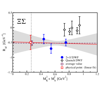
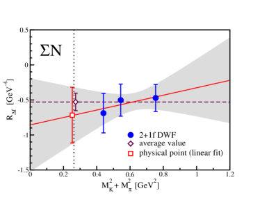
Figure 3: Chiral extrapolation of $R_{\Delta f}$ for $\Xi\rightarrow\Sigma$ (left) and $\Sigma\rightarrow N$ (right). In each panel, solid and dashed lines represent the fitting results obtained by a linear and a constant fit, respectively. The dotted vertical lines mark the position of the physical point. The open square (circle) symbols, which have been shifted slightly to the left (right), represent the extrapolated values at the physical point. In the right panel, quenched DWF results Sasaki:2008ha are also included as open diamonds for a comparison.

where the leading symmetry-breaking correction, which is predicted by the Ademollo-Gatto theorem, is explicitly factorized out. The remaining dependence related to either the higher order corrections of the SU(3) breaking or simulated pion and kaon masses is hardly observed within the statistical errors as shown in Fig. 3.

Indeed, if we simply adopt a linear fit form on $\Delta R$ as a function of $M_{K}^{2}+M_{\pi}^{2}$ to extrapolate the value at the physical point:

$$R_{\Delta f}(M_{K},M_{\pi})=R_{0}+R_{1}\cdot(M_{K}^{2}+M_{\pi}^{2}),$$ (5)

the resulting coefficient $R_{1}$, which is approximately zero, ensures that the remaining dependence of either $M_{K}$ or $M_{\pi}$ is negligible at least within the current statistics. This observation suggests that although the simulated strange quark mass is slightly heavier than the physical mass, the corresponding systematic error is likely to be small in the chiral extrapolation of $R_{\Delta f}$.

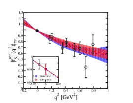
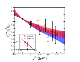
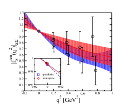
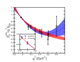
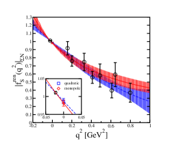
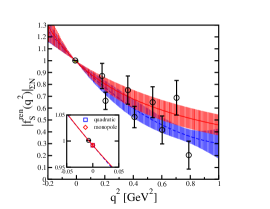
Figure 2: Interpolation of $f_{S}(q^{2})$ to $q^{2}=0$. The upper (lower) panels are for $\Xi\rightarrow\Sigma$ ($\Sigma\rightarrow N$) decay at $am_{ud}=0.005$ (left), 0.01 (middle), and 0.02 (right). Open circles are $|f_{S}(q^{2})|$ at the simulated $q^{2}$. The solid (dashed) curve is the fitting result by using monopole (quadratic) interpolation form, while the open diamond (square) represents the interpolated value to $q^{2}=0$.

We may rather use fitting the data of $R_{\Delta f}$ to a constant to estimate the value at the physical point. The two fits are mutually consistent, but the latter provides the smaller error as shown in Fig. 3. All fitted results are also tabulated in Table 4 as well as the values of $R_{\Delta f}$ given at all simulated quark masses. We thus quote the value of $R_{\Delta f}$ at the physical point:

$$R_{\Delta f}(M_{K}^{\rm phys},M_{\pi}^{\rm phys})=\left\{\begin{array}[]{ll}-0.524(77)&{\rm for}\;\Xi\rightarrow\Sigma\cr-0.529(125)&{\rm for}\;\Sigma\rightarrow N,\end{array}\right.$$ (6)

in $({\rm GeV})^{-4}$, which is obtained from the latter fit, as our best estimate. We evaluate the SU(3)-breaking correction $\Delta f$ via Eq. (4) together with the physical kaon and pion masses and then get

$$\tilde{f}^{\rm AGT}_{1}(0)=1+\Delta f=\left\{\begin{array}[]{ll}0.9737(39)&{\rm for}\;\Xi\rightarrow\Sigma\cr 0.9734(63)&{\rm for}\;\Sigma\rightarrow N,\end{array}\right.$$ (7)

which we call the AGT fit result hereafter. Alternatively, we may perform a global fit of the data on $\tilde{f}_{1}(0)$ as multiple functions of $M_{K}^{2}-M_{\pi}^{2}$ and $M_{K}^{2}+M_{\pi}^{2}$

$$\tilde{f}_{1}(0)=C_{0}+\left(C_{1}+C_{2}\cdot(M_{K}^{2}+M_{\pi}^{2})\right)\cdot(M_{K}^{2}-M_{\pi}^{2})^{2},$$ (8)

whose form is motivated by the AGT fit. Our simulations are performed with a strange quark mass slightly heavier than the physical mass. To take into account this slight deviation in this global analysis of the chiral extrapolation, we simply evaluate a correction using the Gell-Mann-Oakes-Renner relation for the pion and kaon masses, which corresponds to the quark mass dependence of pseudo-scalar meson masses at the leading order of ChPT. This correction could be accurate in as much as the ratio of $R_{\Delta f}$ have shown neither any higher-order corrections of SU(3) breaking nor the remaining $M_{K}$ and $M_{\pi}$ dependences.

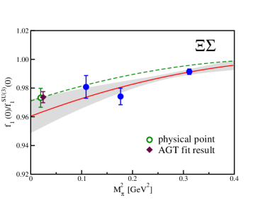
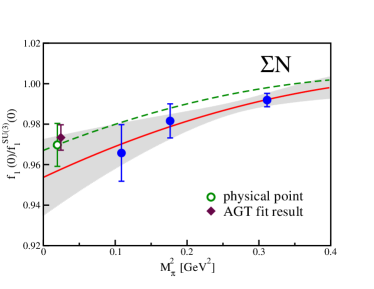
Figure 4: Chiral extrapolation of $\tilde{f}_{1}(0)$ for $\Xi\rightarrow\Sigma$ (left) and $\Sigma\rightarrow N$ (right). In each panel, the filled circles denote our results obtained with the three ensembles, while open circles are extrapolated results at the physical point using a global fitting procedure described in the text. Fitting curves indicated by dashed and solid curves represent the fitting results for the physical strange mass and the simulated one ($am_{s}=0.04$), respectively. The AGT fit results are also included as filled diamond symbols, which have been moved slightly to the right, for comparison.

In Fig. 4, we present the results of $\tilde{f}_{1}(0)$ (filled circles) as a function of the pion mass squared for $\Xi\rightarrow\Sigma$ (left panel) and $\Sigma\rightarrow N$ (right panel). In each panel, fitting curves indicated by dashed and solid curves represent the fitting results with and without the correction for the strange quark mass, respectively. The extrapolated results of $\tilde{f}_{1}(0)$ at the physical point, which are denoted as open circles, agree very well with the AGT fit results indicated by filled diamond symbols. Both results are tabulated in Table 5 together with the data calculated at all simulated quark masses. The statistical errors from the AGT fit are rather smaller than those of the global fits.

Table 3: Results for $|f^{\rm ren}_{S}(q_{\rm max}^{2})|$, where $q_{\rm max}^{2}=-(M_{B_{1}}-M_{B_{2}})^{2}$ with $(B_{1},B_{2})=(\Xi,\Sigma)$ and $(\Sigma,N)$.

	$\Xi\rightarrow\Sigma$		$\Sigma\rightarrow N$
$m_{ud}$	$q_{\rm max}^{2}$ [${\rm GeV}^{2}$]	$|f^{\rm ren}_{S}(q_{\rm max}^{2})|$	$q_{\rm max}^{2}$ [${\rm GeV}^{2}$]	$|f^{\rm ren}_{S}(q_{\rm max}^{2})|$
0.005	$-0.0103(16)$	0.9879(71)	$-0.0360(30)$	1.0166(112)
0.01	$-0.0063(15)$	0.9795(55)	$-0.0223(28)$	1.0108(39)
0.02	$-0.0019(4)$	0.9928(16)	$-0.0080(7)$	1.0013(6)

Table 4: Results for $R_{\Delta f}$ in $({\rm GeV})^{-4}$.

$m_{ud}$	$\Xi\rightarrow\Sigma$	$\Sigma\rightarrow N$
0.005	$-0.386(159)$	$-0.689(281)$
0.01	$-0.706(160)$	$-0.503(229)$
0.02	$-0.501(114)$	$-0.472(193)$
physical point (linear)	$-0.498(243)$	$-0.717(398)$
physical point (average)	$-0.524(77)$	$-0.529(125)$

The excellent agreement observed here between two different fitting procedures indicates that the systematic uncertainty stemming from the small deviation of the strange quark mass appears to be relatively small in the AGT fit, where we directly insert the physical kaon and pion masses into Eq. (4) with the weighted average of $R_{\Delta f}$ in order to determine $\tilde{f}_{1}(0)$ at the physical point. However, we conservatively quote the global fit results as our final estimates. The differences between two determinations may be regarded as the reliability of the extrapolation to the physical point in our current uncertainty. Hence our final results are

$$f_{1}(0)=\left\{\begin{array}[]{ll}+0.9732(66)(7)(5)&{\rm for}\;\Xi\rightarrow\Sigma\cr-0.9698(106)(15)(36)&{\rm for}\;\Sigma\rightarrow N,\end{array}\right.$$ (9)

where the first error is statistical, and the second and third are estimates of the systematic errors due to our choice of $q^{2}$ interpolation and the reliability of the extrapolation to the physical point, respectively. Note that since we simulate at a single lattice spacing, the systematic error introduced by the lattice discretization is not estimated there.

It is worth emphasizing that the signs of the second-order corrections on $f_{1}(0)$ are consistent with what was reported in earlier quenched lattice studies Guadagnoli:2006gj ; Sasaki:2008ha and preliminary results from mixed action calculation Lin:2008rb and $n_{f}=2+1$ dynamical improved Wilson fermion calculations Gockeler:2011se . However, we recall that the tendency of the SU(3)-breaking correction observed here disagrees with predictions of both the latest baryon ChPT result Geng:2009ik and large $N_{c}$ analysis Flores-Mendieta:1998ii ; FloresMendieta:2004sk .

We additionally remark that the latter has received some criticism from Mateu and Pich Mateu:2005wi . They pointed out that the large $N_{c}$ fit including second-order SU(3)-breaking effects on $f_{1}(0)$ becomes unreliable within the present experimental uncertainties .

Table 5: Results for $[f_{1}(0)/f^{\rm SU(3)}_{1}(0)]_{\Xi\rightarrow\Sigma}$ and $[f_{1}(0)/f^{\rm SU(3)}_{1}(0)]_{\Sigma\rightarrow N}$, where $f^{\rm SU(3)}_{1}(0)=+1$ for $\Xi\rightarrow\Sigma$ and $f^{\rm SU(3)}_{1}(0)=-1$ for $\Sigma\rightarrow N$. The final column gives the global fit results for the physical strange mass.

		$m_{ud}$			physical point
	$q^{2}$ interpolation	0.005	0.01	0.02	AGT fit	Global fit
$[f_{1}(0)/f^{\rm SU(3)}_{1}(0)]_{\rm\Xi\rightarrow\Sigma}$	monopole	0.9808(79)	0.9742(58)	0.9914(19)	0.9737(39)	0.9732(66)
	quadratic	0.9806(81)	0.9744(57)	0.9910(19)	0.9730(38)	0.9731(67)
$[f_{1}(0)/f^{\rm SU(3)}_{1}(0)]_{\rm\Sigma\rightarrow N}$	monopole	0.9656(140)	0.9816(84)	0.9919(33)	0.9734(63)	0.9698(106)
	quadratic	0.9641(140)	0.9870(74)	0.9918(31)	0.9759(57)	0.9748(99)

IV Summary

We have studied the flavor SU(3)-breaking effect on hyperon vector coupling $f_{1}(0)$ for the $\Xi^{0}\rightarrow\Sigma^{+}$ and $\Sigma^{-}\rightarrow n$ decays in (2+1)-flavor QCD using domain wall quarks. We have observed that the second-order correction on $f_{1}(0)$ is still negative for both decays at simulated pion masses of $M_{\pi}=330-558$ MeV. The size of the second-order corrections observed here is also comparable to what was observed in our DWF calculations of $K_{l3}$ decays Boyle:2007qe . Using the best estimate of $|V_{us}|=0.2254(6)$ with imposing CKM unitarity Antonelli:2010yf , we then predict the values $|V_{us}f_{1}(0)|_{\Xi\rightarrow\Sigma}=0.2194(8)_{V_{us}}(15)_{f_{1}}$ and $|V_{us}f_{1}(0)|_{\Sigma\rightarrow N}=0.2186(8)_{V_{us}}(24)_{f_{1}}$. The former is barely consistent with a single experimental result of $|V_{us}f_{1}(0)|_{\Xi\rightarrow\Sigma}=0.209(27)$ AlaviHarati:2001xk , albeit with its large experimental error. However, the latter is slightly deviated from the currently available experimental result of $|V_{us}f_{1}(0)|_{\Sigma\rightarrow N}=0.2282(49)$ Cabibbo:2003cu due to reaching the value of $f_{1}(0)$ with an accuracy of less than one percent. We plan to extend our research to evaluate the systematic uncertainty due to the lattice discretization error and also to decrease the reliance on the chiral extrapolation using RBC/UKQCD 2+1 flavor DWF dynamical ensembles at a second, finer, lattice spacing with simulated pion masses closer to the physical point.

- (1) C. Sachrajda, PoS LATTICE 2010, 018 (2010).
- (2) E. Blucher and W. J. Marciano, “, , Cabibbo Angle, and CKM Unitarity,” in J. Beringer et al. (Particle Data Group), Phys. Rev. D 86, 010001 (2012).
- (3) For a review of hyperon beta decays, see N. Cabibbo, E. C. Swallow and R. Winston, Ann. Rev. Nucl. Part. Sci. 53, 39 (2003) and references therein.
- (4) V. Mateu and A. Pich, JHEP 0510, 041 (2005).
- (5) A. Garcia and P. Kielanowski, Lect. Notes Phys. 222, 1 (1985).
- (6) J. M. Gaillard and G. Sauvage, Ann. Rev. Nucl. Part. Sci. 34, 351 (1984).
- (7) D. Guadagnoli, V. Lubicz, M. Papinutto and S. Simula, Nucl. Phys. B 761, 63 (2007).
- (8) S. Sasaki and T. Yamazaki, Phys. Rev. D 79, 074508 (2009).
- (9) S. Weinberg, Phys. Rev. 112, 1375 (1958).
- (10) M. Ademollo and R. Gatto, Phys. Rev. Lett. 13, 264 (1964).
- (11) J. F. Donoghue and B. R. Holstein, Phys. Rev. D25, 206 (1982).
- (12) J. F. Donoghue, B. R. Holstein and S. W. Klimt, Phys. Rev. D 35, 934 (1987).
- (13) F. Schlumpf, Phys. Rev. D 51, 2262 (1995).
- (14) R. Flores-Mendieta, E. Jenkins and A. V. Manohar, Phys. Rev. D 58, 094028 (1998).
- (15) G. Villadoro, Phys. Rev. D 74, 014018 (2006).
- (16) A. Lacour, B. Kubis and U. G. Meissner, JHEP 0710, 083 (2007).
- (17) L. S. Geng, J. Martin Camalich and M. J. Vicente Vacas, Phys. Rev. D 79, 094022 (2009).
- (18) C. Allton et al. [RBC-UKQCD Collaboration], Phys. Rev. D 78, 114509 (2008).
- (19) T. Yamazaki et al. [RBC+UKQCD Collaboration], Phys. Rev. Lett. 100, 171602 (2008).
- (20) T. Yamazaki et al. [RBC+UKQCD Collaboration], Phys. Rev. D 79, 114505 (2009).
- (21) Y. Aoki et al. [RBC+UKQCD Collaboration], Phys. Rev. D 82, 014501 (2010).
- (22) S. Sasaki, AIP Conf. Proc. 1388 (2011) 443-446; arXiv:1102.4934 [hep-lat].
- (23) S. Sasaki, K. Orginos, S. Ohta and T. Blum, [RIKEN-BNL-Columbia-KEK Collaboration], Phys. Rev. D 68, 054509 (2003).
- (24) H. W. Lin, Nucl. Phys. Proc. Suppl. 187, 200 (2009).
- (25) M. Gockeler et al. [QCDSF Collaboration and UKQCD Collaboration], PoS LATTICE2010, 165 (2010).
- (26) R. Flores-Mendieta, Phys. Rev. D 70, 114036 (2004).
- (27) P. A. Boyle et al. [RBC+UKQCD Collaboration], Phys. Rev. Lett. 100, 141601 (2008).
- (28) M. Antonelli, V. Cirigliano, G. Isidori, F. Mescia, M. Moulson, H. Neufeld, E. Passemar, M. Palutan, et al., Eur. Phys. J. C 69, 399 (2010).
- (29) A. Alavi-Harati et al. [KTeV Collaboration], Phys. Rev. Lett. 87, 132001 (2001).