Superiorization of EM Algorithm and Its Application in Single-Photon Emission Computed Tomography(SPECT)

Abstract

In this paper, we presented an efficient algorithm to implement the regularization reconstruction of SPECT. Image reconstruction with priori assumptions is usually modeled as a constrained optimization problem. However, there is no efficient algorithm to solve it due to the large scale of the problem. In this paper, we used the superiorization of the expectation maximization (EM) iteration to implement the regularization reconstruction of SPECT. We first investigated the convergent conditions of the EM iteration in the presence of perturbations. Secondly, we designed the superiorized EM algorithm based on the convergent conditions, and then proposed a modified version of it. Furthermore, we gave two methods to generate desired perturbations for two special objective functions. Numerical experiments for SPECT reconstruction were conducted to validate the performance of the proposed algorithms. The experiments show that the superiorized EM algorithms are more stable and robust for noised projection data and initial image than the classic EM algorithm, and outperform the classic EM algorithm in terms of mean square error and visual quality of the reconstructed images.

Keywords: EM algorithm, superiorization, SPECT.

1 Introduction

Single-photon emission computed tomography (SPECT), which can visualize the physiological information of various organs with the help of radiopharmaceuticals [1, 2, 3], a biochemical molecule labeled with radioactivity. The gamma-rays emitted by the injected radioactive material are recorded by a gamma camera rotated around the patient. The goal of SPECT is to reconstruct the radionuclide distribution from the measurements numerically. The variety of existing SPECT reconstruction algorithms can be split into a family of analytical methods [4, 5, 6, 7, 8] and a wide class of iterative techniques [9, 10, 11].
From the analytic point of view, the SPECT reconstruction problem [3, 4, 7] is to invert the attenuated Radon transform(aRt) of $f$(distribution of radiopharmaceutical)

$$R_{a}f(s,\varphi)=\int_{R}f(s\theta+t\theta^{\perp})e^{-\int_{t}^{\infty}\mu(s\theta+\tau\theta^{\perp}){d\tau}}dt,$$ (1)

where $\mu$ is a known function, referred to as the attenuation map of gamma-rays, $\theta=(\cos\varphi,\sin\varphi)$ and $\theta^{\perp}=(-\sin\varphi,\cos\varphi)$. In practice, $f$ and $\mu$ are two functions with compact support $\Omega$. Therefore, the integrand in (1) is zero outside a bounded interval, and this integral is written over $(-\infty,+\infty)$ for convenience.
For the iterative methods, the SPECT reconstruction problem is to solve the following linear system [9],

$$Ax=b,$$ (2)

where the elements of the observed data $b=(b_{1},b_{2}\cdots,b_{M})^{t}\in\mathbb{R}^{M}$, the unknown image $x=(x_{1},x_{2}\cdots,x_{N})^{t}\in\mathbb{R}^{N}$ and the system matrix $A=(a_{ij})\in\mathbb{R}^{M\times N}$ are all nonnegative. Here and in the following, the superscript ^t denotes the transpose of vector. The aim is to reconstruct the unknown $x$ as an image from the projection data $b$ via stable algorithms. A solution is not feasible with conventional methods directly because of the noisy projection data $b$, the ill-posedness and large scale of the problem. For the SPECT reconstruction, the system matrix $A$ not only can model the attenuation of the gamma-rays, but also can fuse some realistic factors, such as photon scattering and camera blurring.
The expectation maximization (EM) algorithm [9, 12] and the algebraic reconstruction technique (ART)[13, 14] are two widely used technologies in imaging sciences, due to their simplicity, efficiency and performance. In practice, the EM algorithm is more appropriate for emission tomography including SPECT. Firstly, the EM algorithm maintains the nonnegative constraint in the iteration procedure. Secondly, the EM algorithm is relatively robust against data inconsistencies introduced by Poisson noise, because it seeks to minimize the Kullback-Liebler(K-L) distance between the measured data $b$ and the projection of the estimated image $Ax$, which is equivalent to maximizing the likelihood of Poisson distribution.
For SPECT reconstruction, it is one of the main issues to estimate the radionuclide distribution from low-counts projection data. This issue occurs quite frequently because of practical constraints, such as imaging hardware and scanning geometry. Furthermore, in order to reduce acquisition time, radiation dose and imaging cost efficiently, we should decrease the counts of the projection data. However, this would cause the strong deterioration of the observed data and the under-determinacy ($m\ll n$) of the linear system (2). In these situations, the reconstructed images by the EM algorithm are usually dominated by various distortions, because the EM algorithm accepts any solution which minimizes the K-L distance and depends on the initial point.
The qualities of the reconstructed images can be improved by regularization reconstruction methods. Regularization methods are often used techniques to improve the quality of reconstructed images. There are two regularization reconstruction models: unconstraint optimization[15, 16, 17, 18, 19, 20]

$$\min_{x}\{\phi(x)+{1\over\lambda}{D(b,Ax)}\}$$ (3)

and constraint optimization [21, 22, 23]

$$\min\phi(x)\text{\quad s.t.\quad}x\in\{x|D(b,Ax)<\epsilon\}$$ (4)

where $\phi$ is a convex function, representing the prior knowledge. $D(\cdot,\cdot)$ denotes a distance function, such as $l^{2}$ and K-L distances. The parameters $\lambda,\epsilon$ are nonnegative and related to the noise level. The lower the noise level is, the smaller the parameters are.
For the first optimization problem (3), there are different algorithms [17, 18, 20, 24]. In this paper, we focus on the second optimization problem (4). To our knowledge, there is no optimal algorithm to solve the constraint optimization problem (4) efficiently due to the large scale. In this paper, we resort to an emerging approach called superiorization [25] to implement the regularization reconstruction of SPECT.
The superiorization of iterative methods, which was first proposed by the authors of [21], is a relaxation technology for the constrained optimization problem. The superiorized algorithm lies between the feasibility-seeking algorithms, which seek a feasible point in the constrained set, and the optimal algorithms, which seek the minimum point of objective function in the constrained set. The aim of superiorization algorithm is to look for a superior instead of the optimal point of the objective function or just a feasible point in the constrained set. The basic idea of superiorization is to do the feasibility-seeking algorithms with perturbations about the objective function.
The superiorization of ART algorithms has been studied and applied to the regularization reconstruction of computed tomography(CT) [21, 22, 25, 26, 27]. The authors of [21, 26] first investigated the convergence of the two variants of ART under summable perturbations for consistent case. For inconsistent case, the authors of [27] proved the convergence of symmetric version of ART in the presence of summable perturbations. The superiorization of the EM algorithm was firstly proposed in [28], and applied to bioluminescence tomography. However, to our knowledge, it is still an open problem about the convergence of the superiorized EM algorithm.
In this paper, we first discussed the convergence of the EM algorithm in the presence of perturbation in section 2. A so-called bounded perturbation resilient (BPR) property of ART is vital in the proof of convergence for the perturbed version of ART. However, we cannot prove the BPR property of the EM iteration so far, because of the nonlinearity of the EM operator. Therefore, we investigated the convergence of the perturbed EM algorithm under the following assumptions. Firstly, the perturbations should maintain the positivity of iterations. Secondly, the perturbations should go to zero with the increase of iterates. Lastly, the perturbed EM iteration should gradually decrease the K-L distance between the observed data and the projection of estimation by each iteration.
Based on the convergent conditions, we presented the superiorized EM algorithm and its modified version in section 3. Furthermore, practicable techniques were given to produce ideal perturbations for two special objective functions, total variation(TV) [29] and $l^{1}$-norm [30], widely used in imaging sciences. While the proposed algorithms are applicable to diverse inverse problems, in this paper we restricted ourselves to demonstrate its usefulness to the SPECT reconstruction. Numerical results for SPECT reconstruction were given in section 4. As our expectation, the superiorization algorithms output superior image comparing with the classic EM algorithm in terms of MSE and visual quality. Some conclusions and discussions were given in section 5.

2 Perturbations Resilience of EM Iteration

For the sake of reference, we first introduce some notations and assumptions. In this paper, an image $x$ is described as a vector of length $N$ with individual elements $x_{j}$, $j=1,2,\cdots,N$. When it is necessary to refer to pixels in the context of a two-dimensional (2D) image we use the double subscript form $x_{p,q}$ , where

$$j=(q-1)W+p,p=1,2,\cdots,H,q=1,2,\cdots,W,$$ (5)

and integers $W$ and $H$ are, respectively, the width and height of the 2D image array, which has a total number of pixels $N=W\times H$. Denote by $\mathbb{R}^{N}_{+}$ the region $\{x\geq 0|x\in\mathbb{R}^{N}\}$. For the system matrix $A$, we set $H_{j}=\sum_{i=1}^{M}a_{ij}$ and $d_{i}(x)=\sum_{j=1}^{N}a_{ij}x_{j}$ for convenience. Furthermore, we introduce

$$g_{ij}(x) = \frac{a_{ij}b_{i}}{d_{i}(x)},$$ (6)

and

$$f_{j}(x) = {1\over H_{j}}\sum_{i=1}^{M}\frac{a_{ij}b_{i}}{d_{i}(x)}={1\over H_{j}}\sum_{i=1}^{M}g_{ij}(x).$$ (7)

Let $P$ denote the EM operator, and then the EM iteration $x^{k+1}=P(x^{k})=(P_{1}(x^{k}),\cdots,P_{N}(x^{k}))^{t}$ for the problem (2) is defined as

$$x^{k+1}_{j} = P_{j}(x^{k})={x^{k}_{j}\over H_{j}}\cdot\sum\limits_{i=1}^{M}{b_{i}a_{ij}\over{\sum_{t=1}^{N}a_{it}x_{t}^{k}}}=x_{j}^{k}\cdot f_{j}(x^{k}),$$ (8)

with an initial image $x^{0}>0$. Similarly, the perturbed version of the EM iteration is defined as

$$x^{k+1}_{j}=P_{j}(x^{k}+\beta_{k}v^{k})={y^{k}_{j}\over H_{j}}\cdot\sum_{i=1}^{M}\frac{b_{i}a_{ij}}{\sum_{t=1}^{N}a_{it}y^{k}_{t}}=y^{k}_{j}\cdot f_{j}(y^{k}),$$ (9)

where $y^{k}=x^{k}+\beta_{k}v^{k}$. Here, the vector $v^{k}\in\mathbb{R}^{N}$ and number $\beta_{k}\geq 0$ represent the direction and length of the perturbation of the $k$th iteration, respectively. Hereafter, we call the EM iteration without perturbation as the classic EM iteration to distinguish from each other.
It has been established that the sequence $\{x^{n}\}$ generated by the classic EM iteration converges to a minimizer of the K-L distance $I_{A}^{b}(x)$ between $b$ and $Ax$ on $R_{+}^{N}$, where $I_{A}^{b}(x)$ is defined as

$$I_{A}^{b}(x) = I(b,Ax)=\sum\limits_{i=1}^{M}b_{i}\ln\frac{b_{i}}{d_{i}(x)}-\sum\limits_{i=1}^{M}(b_{i}-d_{i}(x)),$$ (10)

where $I(\cdot,\cdot)$ denote the K-L distance function of any two nonnegative vectors. An important inequality used in this paper is

$$\ln t\geq 1-{1\over t},$$ (11)

for $t>0$, and the inequality holds with equality if and only if $t=1$. By using the inequality (11), we have that $I(x,y)\geq 0$ for all vectors $x,y\geq 0$, and the inequality holds with equality if and only if $x=y$.
Obviously, if $\beta_{k}=0$, the perturbed EM iteration is the same as the classic EM iteration, in which we are not interested. Therefore, in the following we assume $\beta_{k}>0$. A natural question is that under what assumptions the sequence $\{x^{n}\}$ generated by the perturbed EM iteration (9) converges to a minimizer of (10) as well. Before discussing the convergent conditions of the perturbed EM iteration, we first summarize some propositions of the classic EM iteration [9, 12, 31]. Without loss of generality, we assume that all the elements $b_{i}>0$ for all $i$, and $H_{j}=\sum_{i=1}^{M}a_{ij}=1$ for all $j$ for simplicity.

Theorem 2.1

For any initial image $x^{0}>0$, denote by $x^{k}$ the estimate of the classic EM algorithm after $k$ iterations. Then the following propositions hold:

1. $x^{k}>0$ and $\sum_{j=1}^{N}x_{j}^{k}=\sum_{i=1}^{M}b_{i}$, for all $k>0$.

2. $I_{A}^{b}(x^{k+1})\leq I_{A}^{b}(x^{k})$, and $I(x^{k+1},x^{k})\leq I_{A}^{b}(x^{k})-I_{A}^{b}(x^{k+1})$.

3. $\{x^{k}\}$ converges to a minimizer $x^{\ast}$ of $I_{A}^{b}(x)$ on $\mathbb{R}_{+}^{N}$, and $x^{\ast}$ is a fixed point of the EM operator.

4. $I(x^{\ast},x^{k+1})\leq I(x^{\ast},x^{k})$.

The inequalities in second and fourth items above hold with equalities if and only if $x^{k}$ is a fixed point of the EM operator.

Remark 2.2

Obviously, $x$ is a fixed point of the EM operator if and only if $f_{j}(x)=1$ for $x_{j}\neq 0$.

From the propositions above, we have that the sequence $\{I_{A}^{b}(x^{k})\}$ monotonically converges to the minimum of $I_{A}^{b}(\cdot)$ on $\mathbb{R}_{+}^{N}$, and $\{x^{k}\}$ approximates to the minimizer $x^{\ast}$ gradually. Next, we investigate the convergence of the perturbed EM iteration, and prove the similar propositions as far as we can.

Theorem 2.3

Given any initial image $x^{0}$, denote by $\{x^{k}\}_{k\in\mathbb{N}}$ the sequence generated by the perturbed EM iteration (9).

$$x^{k+1}_{j} = ({x_{j}^{k}+\beta_{k}{v^{k}_{j}}})\cdot f_{j}(x^{k}+\beta_{k}v^{k})={{y^{k}_{j}}}\cdot f_{j}(y^{k}),$$ (12)

where $y_{j}^{k}=x^{k}_{j}+\beta_{k}v_{j}^{k}$, and $\{v^{k}\}$ is a bounded sequence. Suppose that

1. Positivity: $y_{j}^{k}>0$.

2. Vanishing: $\beta_{k}\longrightarrow 0$.

3. Decreasing

   $$\beta_{k}\max_{j\in{S_{k}^{-}}}\{-\frac{v_{j}^{k}}{y_{j}^{k}}\}B_{k}^{-}-\beta_{k}\min_{j\in{S_{k}^{+}}}\{\frac{v_{j}^{k}}{y_{j}^{k}}\}B_{k}^{+}+\beta_{k}\sum_{j=1}^{N}v_{j}^{k} < I_{A}^{b}(y^{k})-I_{A}^{b}(x^{k+1}),$$ (13)

   where $S^{-}_{k}=\{j|v_{j}^{k}<0\},S^{+}_{k}=\{j|v_{j}^{k}>0\}$ , and $B_{k}^{-}=\max\{\rho+\sum_{j\in{S_{k}^{-}}}x_{j}^{k+1},\sum_{j\in{S_{k}^{-}}}\hat{x}_{j}\}$, $B_{k}^{+}=\min\{\sum_{j\in{S_{k}^{+}}}x_{j}^{k+1},\sum_{j\in{S_{k}^{+}}}\hat{x}_{j}\}$. Here $\rho$ is a sufficiently small positive number.

Then, the following propositions hold:

1. $I_{A}^{b}(x^{k+1})\leq I_{A}^{b}(x^{k})$.

2. $\{x^{k}\}$ has a convergent subsequence $\{x^{m_{k}}\}$, and the limit $\hat{x}$ is a fixed point of the EM operator.

3. $I(\hat{x},x^{k+1})\leq I(\hat{x},x^{k})$, and $x^{k}\longrightarrow\hat{x}$.

4. $\hat{x}$ is a minimizer of $I_{A}^{b}(x)$.

Furthermore, the inequalities above hold with equalities iff $x^{k}$ is a fixed point of the EM operator and $\beta_{k}v^{k}=0$.

Before presenting the proof, we explain the necessities of the conditions of theorem 2.3. The positive condition of $y_{j}^{k}$ is necessary for the nonnegative constraints. The second condition is required by the convergence of the sequence $\{x^{k}\}$. Intuitively, the last condition is used to guarantee that $I_{A}^{b}(x^{k+1})\leq I_{A}^{b}(x^{k})$, which implies the convergence of $I_{A}^{b}(x^{k})$.
An important concern is about the existence of the perturbations satisfying the conditions of theorem 2.3, especially the third condition. Because the sequence $\{\hat{x}^{k}\}$ generated by the classic EM iteration ($\beta_{k}=0$) satisfies the conditions in theorem 2.3, the sequence $\{x^{k}\}$ generated by the perturbed version also satisfies them when $\beta_{k}$s are small enough for each iteration due to the continuities of the EM operator (9) and K-L distance (10). Therefore, there exist perturbations which satisfy the assumptions of theorem 2.3.
Proof : We prove this theorem step by step, which follows the proving procedure in [31].

1. Proof of proposition 1: By the definition of $I_{A}^{b}(\cdot)$ and $d_{i}(\cdot)$, we have

   $$I_{A}^{b}(x^{k})-I_{A}^{b}(x^{k+1})$$

   $$= \sum_{i=1}^{M}b_{i}\ln\frac{b_{i}}{d_{i}(x^{k})}-\sum_{i=1}^{M}b_{i}\ln\frac{b_{i}}{d_{i}(x^{k+1})}$$

   $$= \sum_{i=1}^{M}b_{i}\ln\frac{d_{i}(x^{k+1})}{d_{i}(y^{k})-\beta_{k}d_{i}(v^{k})}$$

   $$= \sum_{i=1}^{M}b_{i}\ln\frac{d_{i}(x^{k+1})}{d_{i}(y^{k})}+\sum_{i=1}^{M}b_{i}\ln\frac{1}{1-\beta_{k}d_{i}(v^{k})/d_{i}(y^{k})}$$

   $$\geq I_{A}^{b}(y^{k})-I_{A}^{b}(x^{k+1})-\beta_{k}\sum_{j=1}^{N}v_{j}^{k}+\sum_{i=1}^{M}b_{i}\left[1-\left(1-\beta_{k}\frac{d_{i}(v^{k})}{d_{i}(y^{k})}\right)\right]$$

   $$= I_{A}^{b}(y^{k})-I_{A}^{b}(x^{k+1})-\beta_{k}\sum_{j=1}^{N}v_{j}^{k}+\sum_{i=1}^{M}b_{i}\beta_{k}\frac{d_{i}(v^{k})}{d_{i}(y^{k})}$$

   $$\geq \beta_{k}\max_{j\in{S_{k}^{-}}}\{-\frac{v_{j}^{k}}{y_{j}^{k}}\}B_{k}^{-}-\beta_{k}\min_{j\in{S_{k}^{+}}}\{\frac{v_{j}^{k}}{y_{j}^{k}}\}B_{k}^{+}+\beta_{k}\sum_{i=1}^{M}b_{i}\frac{d_{i}(v^{k})}{d_{i}(y^{k})}$$

   $$= \beta_{k}\max_{j\in{S_{k}^{-}}}\{-\frac{v_{j}^{k}}{y_{j}^{k}}\}B_{k}^{-}-\beta_{k}\min_{j\in{S_{k}^{+}}}\{\frac{v_{j}^{k}}{y_{j}^{k}}\}B_{k}^{+}+\beta_{k}\sum_{j=1}^{N}\frac{v_{j}^{k}}{y_{j}^{k}}y_{j}^{k}\sum_{i=1}^{M}\frac{a_{ij}b_{i}}{d_{i}(y^{k})}$$

   $$= \beta_{k}\max_{j\in{S_{k}^{-}}}\{-\frac{v_{j}^{k}}{y_{j}^{k}}\}B_{k}^{-}-\beta_{k}\min_{j\in{S_{k}^{+}}}\{\frac{v_{j}^{k}}{y_{j}^{k}}\}B_{k}^{+}+\beta_{k}\sum_{j=1}^{N}\frac{v_{j}^{k}}{y_{j}^{k}}x^{k+1}_{j}$$

   $$\geq \beta_{k}\max_{j\in{S_{k}^{-}}}\{-\frac{v_{j}^{k}}{y_{j}^{k}}\}(B_{k}^{-}-\sum_{j\in{S_{k}^{-}}}x^{k+1}_{j})-\beta_{k}\min_{j\in{S_{k}^{+}}}\{\frac{v_{j}^{k}}{y_{j}^{k}}\}(B_{k}^{+}-\sum_{j\in{S_{k}^{+}}}x^{k+1}_{j})$$

   $$\geq \beta_{k}\max_{j\in{S_{k}^{-}}}\{-\frac{v_{j}^{k}}{y_{j}^{k}}\}\rho-\beta_{k}\min_{j\in{S_{k}^{+}}}\{\frac{v_{j}^{k}}{y_{j}^{k}}\}(B_{k}^{+}-\sum_{j\in{S_{k}^{+}}}x^{k+1}_{j}).$$ (15)

   The first and second inequalities hold because of the inequality (11) and the condition (13), respectively. Therefore, we have proved that $I_{A}^{b}(x^{k+1})\leq I_{A}^{b}(x^{k})$ by (13) and (15).
   Finally, we should prove that $I_{A}^{b}(x^{k+1})=I_{A}^{b}(x^{k})$ iff $\beta_{k}v^{k}=0$ and $x^{k}$ is a fixed point of EM operator. The sufficiency is obvious by theorem 2.1. The necessity is also true by the following facts. If $I_{A}^{b}(x^{k+1})=I_{A}^{b}(x^{k})$, we have that all the inequalities in the derivation above hold with equalities, which implies that $\frac{1}{1-\beta_{k}d_{i}(v^{k})/d_{i}(y^{k})}=1$ for all $i$ and $S^{-}_{k}=\emptyset$ by inequalities (1) and (15), respectively, i.e. $\beta_{k}d_{i}(v^{k})=0$ and $v_{j}^{k}\geq 0$. In fact, we have that $v_{j}^{k}=0(\forall~{}j)$, i.e. $y_{j}^{k}=x_{j}^{k}$, and $x^{k}$ is a fixed point by theorem 2.1. Otherwise, assume $v_{j_{0}}^{k}>0$ for some $j_{0}$, there must exist $i_{0}$ such that $a_{i_{0}j_{0}}>0$ and $d_{i_{0}}(v^{k})=\sum_{j=1}^{N}a_{i_{0}j}v^{k}_{j}\geq a_{i_{0}j_{0}}v_{j_{0}}>0$ by the assumption $\sum_{i=1}^{M}a_{ij}=1\neq 0$, which is contradict to $d_{i}(v^{k})=0(\forall~{}i)$.

2. Proof of proposition 2: Because $0<\sum_{j=1}^{N}x_{j}^{k}=\sum_{i=1}^{M}b_{i}$(constant) and $x^{k}>0$, $\{x^{k}\}$ has a convergent subsequence $\{x^{m_{k}}\}$. Denoting by $\hat{x}$ the limit of $\{x^{m_{k}}\}$, we have $y^{m_{k}}\longrightarrow\hat{x}$ because $\beta_{k}\longrightarrow 0$ and $v^{k}$ is bounded. Next we prove $\hat{x}$ is a fixed point of the EM operator. To this end, we define a function for $x\geq 0$

   $$D(x)=I(P(x),x).$$ (16)

   By the second proposition of theorem 2.1, we have

   $$D(y^{m_{k}})=I(P(y^{m_{k}}),y^{m_{k}})=I(x^{m_{k}+1},y^{m_{k}})\leq I_{A}^{b}(y^{m_{k}})-I_{A}^{b}(x^{m_{k}+1}).$$ (17)

   Due to the proposition 1 of theorem 2.3, $\{I_{A}^{b}(x^{k})\}$ is a convergent sequence. Furthermore, $\{I_{A}^{b}(y^{k})\}$ converges to the same limit as $\{I^{b}_{A}(x^{k})\}$ because of the continuity of $I^{b}_{A}(\cdot)$ and $\beta_{k}\longrightarrow 0$. Therefore, we have $I_{A}^{b}(y^{m_{k}})-I_{A}^{b}(x^{m_{k}+1})\longrightarrow 0$, $m_{k}\longrightarrow\infty$. Thus, we have that

   $$D(\hat{x})=\lim_{m_{k}\longrightarrow\infty}D(y^{m_{k}})=I(P(\hat{x}),\hat{x})=0,$$ (18)

   i.e. $\hat{x}$ is a fixed point of the EM operator, since $I(x,y)=0\Longleftrightarrow x=y$. Therefore, we have $f_{j}(\hat{x})=1$ if $\hat{x}_{j}\neq 0$ by the EM iteration formula.

3. Proof of proposition 3: Before going further, we first prove a general inequality that $I(\hat{x},x)-I(\hat{x},P(x))\geq I_{A}^{b}(x)-I_{A}^{b}(\hat{x})$ for any point $x>0$. Assuming $z=P(x)$, we have

   $$I(\hat{x},x)-I(\hat{x},z)$$ (19)

   $$= \sum_{j=1}^{N}\hat{x}_{j}\ln\frac{\hat{x}_{j}}{x_{j}}-\sum_{j=1}^{N}(\hat{x}_{j}-x_{j})+\sum_{j=1}^{N}\hat{x}_{j}\ln\frac{\hat{x}_{j}}{z_{j}}-\sum_{j=1}^{N}(\hat{x}_{j}-z_{j})$$

   $$= \sum_{j=1}^{N}\hat{x}_{j}\ln\frac{z_{j}}{x_{j}}-\sum_{j=1}^{N}(\hat{x}_{j}-x_{j})$$

   $$= \sum_{j=1}^{N}\hat{x}_{j}\sum_{i=1}^{M}g_{ij}(\hat{x})\ln\frac{z_{j}}{x_{j}}\frac{g_{ij}(x)}{g_{ij}(x)}\frac{g_{ij}(\hat{x})}{g_{ij}(\hat{x})}-\sum_{j=1}^{N}(\hat{x}_{j}-x_{j})$$

   $$= \sum_{j=1}^{N}\hat{x}_{j}\sum_{i=1}^{M}g_{ij}(\hat{x})\ln\frac{z_{j}}{x_{j}}\frac{g_{ij}(\hat{x})}{g_{ij}(x)}+\sum_{j=1}^{N}\hat{x}_{j}\sum_{i=1}^{M}g_{ij}(\hat{x})\ln\frac{g_{ij}(x)}{g_{ij}(\hat{x})}-\sum_{j=1}^{N}(\hat{x}_{j}-x_{j})$$

   $$\geq -\sum_{j=1}^{N}\hat{x}_{j}\ln\sum_{i=1}^{M}g_{ij}(\hat{x})\frac{x_{j}}{z_{j}}\frac{g_{ij}(x)}{g_{ij}(\hat{x})}+\sum_{j=1}^{N}\hat{x}_{j}\sum_{i=1}^{M}g_{ij}(\hat{x})\ln\frac{\frac{a_{ij}b_{i}}{d_{i}(x)}}{\frac{a_{ij}b_{i}}{d_{i}(\hat{x})}}-\sum_{j=1}^{N}(\hat{x}_{j}-x_{j})$$

   $$= -\sum_{j=1}^{N}\hat{x}_{j}\ln\frac{x_{j}f_{j}(x)}{z_{j}}+\sum_{i=1}^{M}\sum_{j=1}^{N}\hat{x}_{j}\frac{a_{ij}b_{i}}{d_{i}(\hat{x})}\ln\frac{d_{i}(\hat{x})}{d_{i}(x)}-\sum_{j=1}^{N}(\hat{x}_{j}-x_{j})$$

   $$= \sum_{i=1}^{M}b_{i}\ln\frac{d_{i}(\hat{x})}{d_{i}(x)}-\sum_{j=1}^{N}(\hat{x}_{j}-x_{j})$$

   $$= \sum_{i=1}^{M}b_{i}\ln\frac{b_{i}}{d_{i}(x)}-\sum_{i=1}^{M}(b_{i}-d_{i}(x))+\sum_{i=1}^{M}(b_{i}-d_{i}(x))$$

   $$-\sum_{i=1}^{M}b_{i}\ln\frac{b_{i}}{d_{i}(\hat{x})}+\sum_{i=1}^{M}(b_{i}-d_{i}(\hat{x}))-\sum_{i=1}^{M}(b_{i}-d_{i}(\hat{x}))-\sum_{j=1}^{N}(\hat{x}_{j}-x_{j})$$

   $$= I_{A}^{b}(x)-I_{A}^{b}(\hat{x})+\sum_{i=1}^{M}(d_{i}(\hat{x})-d_{i}(x))-\sum_{j=1}^{N}(\hat{x}_{j}-x_{j})$$

   $$= I_{A}^{b}(x)-I_{A}^{b}(\hat{x}),$$

   where we used the relationship $\sum_{j=1}^{N}\hat{x}_{j}=\sum_{j=1}^{N}x^{k}_{j}=\sum_{i=1}^{M}b_{i}=\sum_{j=1}^{N}z_{j}$. The inequality and the second equality are implied by Jensen’s inequality and the fact $f_{j}(\hat{x})=\sum_{i=1}^{M}g_{ij}(\hat{x})=1$ for $\hat{x}_{j}\neq 0$, respectively. The last equality follows the fact that

   $$\sum_{i=1}^{M}d_{i}(x)=\sum_{i=1}^{M}\sum_{j=1}^{N}a_{ij}{x}_{j}=\sum_{j=1}^{N}x_{j},$$ (20)

   by the assumption that $\sum_{i=1}^{M}a_{ij}=1$. Let $x=y^{k}$, then $z=P(y^{k})=x^{k+1}$ and $I(\hat{x},y^{k})-I(\hat{x},x^{k+1})\geq I_{A}^{b}(y^{k})-I_{A}^{b}(\hat{x})$ by (19). Furthermore, we have

   $$I(\hat{x},y^{k})-I(\hat{x},x^{k+1}) \geq I_{A}^{b}(y^{k})-I_{A}^{b}(\hat{x})$$ (21)

   $$= \left[I_{A}^{b}(y^{k})-I_{A}^{b}(x^{k+1})\right]+I_{A}^{b}(x^{k+1})-I_{A}^{b}(\hat{x})$$

   $$\geq I_{A}^{b}(y^{k})-I_{A}^{b}(x^{k+1}).$$

   The last inequality holds because $I_{A}^{b}(x^{k+1})\geq I_{A}^{b}(\hat{x})$. Now, we prove $I(\hat{x},x^{k+1})\leq I(\hat{x},x^{k})$. By the definitions of the K-L distance and the perturbed EM iteration, we have

   $$I(\hat{x},x^{k})-I(\hat{x},x^{k+1})$$

   $$= \sum_{j=1}^{N}\hat{x}_{j}\ln\frac{(x_{j}^{k}+\beta_{k}v^{k}_{j})f_{j}(y^{k})}{x^{k}_{j}}$$

   $$= \sum_{j=1}^{N}\hat{x}_{j}\ln{f_{j}(y^{k})}+\sum_{j=1}^{N}\hat{x}_{j}\ln(1+\beta_{k}\frac{v_{j}^{k}}{x_{j}^{k}})$$

   $$\geq \sum_{j=1}^{N}\hat{x}_{j}\ln\frac{y^{k}_{j}f_{j}(y^{k})}{y_{j}^{k}}+\sum_{j=1}^{N}\hat{x}_{j}\left(1-\frac{1}{1+\beta_{k}{v_{j}^{k}}/{x_{j}^{k}}}\right)$$

   $$= I(\hat{x},y^{k})-I(\hat{x},x^{k+1})+\sum_{j=1}^{N}\hat{x}_{j}\frac{\beta_{k}v_{j}^{k}}{x_{j}^{k}+\beta_{k}{v_{j}^{k}}}-\beta_{k}\sum_{j=1}^{N}v_{j}^{k}$$

   $$\geq I_{A}^{b}(y^{k})-I_{A}^{b}(x^{k+1})-\beta_{k}\max_{j\in{S_{k}^{-}}}\{-\frac{v_{j}^{k}}{y_{j}^{k}}\}\sum_{j\in{S_{k}^{-}}}\hat{x}_{j}+\beta_{k}\min_{j\in{S_{k}^{+}}}\{\frac{v_{j}^{k}}{y_{j}^{k}}\}\sum_{j\in{S_{k}^{+}}}\hat{x}_{j}-\beta_{k}\sum_{j=1}^{N}v_{j}^{k}$$

   $$\geq \beta_{k}\max_{j\in{S_{k}^{-}}}\{-\frac{v_{j}^{k}}{y_{j}^{k}}\}(B_{k}^{-}-\sum_{j\in{S_{k}^{-}}}\hat{x}_{j})+\beta_{k}\min_{j\in{S_{k}^{+}}}\{\frac{v_{j}^{k}}{y_{j}^{k}}\}(\sum_{j\in{S_{k}^{+}}}\hat{x}_{j}-B_{k}^{+})$$

   $$\geq 0.$$ (23)

   Again we used the inequality (11) for the first inequality. The second and the last inequalities hold by (21) and (13), respectively. Thus, we have that $I(\hat{x},x^{k+1})\leq I(\hat{x},x^{k})$ by equation (23).
   Next, we need to prove that $I(\hat{x},x^{k+1})=I(\hat{x},x^{k})$ iff $\beta_{k}v^{k}_{j}=0$ and $x^{k}$ is a fixed point of EM operator. The sufficiency is clear. The necessity is also true by the following facts. If $I(\hat{x},x^{k+1})=I(\hat{x},x^{k})$, we have that all the inequalities in the derivation above hold with equalities, which implies that $\beta_{k}v_{j}^{k}=0$ and $I_{A}^{b}(y^{k})=I_{A}^{b}(x^{k+1})$ by inequalities (3) and (23), respectively. Therefore, we have that $y^{k}=x^{k}$ and $x^{k}$ is a fixed point of EM operator by theorem 2.1.
   Finally, we need to prove that $x^{k}\longrightarrow\hat{x}$. Firstly, we have $I(\hat{x},x^{k})\searrow 0$ since $I(\hat{x},x^{m_{k}})\longrightarrow 0$ and the sequence $\{I(\hat{x},x^{k})\}$ monotonously decreases. Therefore, we have proved $x^{k}\longrightarrow\hat{x}$ by $I(x,y)=0\Longleftrightarrow x=y$, and $y^{k}\longrightarrow\hat{x}$ as well by $\beta_{k}v^{k}\longrightarrow 0$.

4. Proof of proposition 4: In order to prove this proposition, we should prove that $\hat{x}$ satisfies the Kuhn-Tucker (K-T) conditions. For the EM algorithm and the K-L function, the K-T conditions are equivalent to (1) $f_{j}(\hat{x})=1$ if $\hat{x}_{j}\neq 0$, and (2) $0\leq f_{j}(\hat{x})\leq 1$ if $\hat{x}_{j}=0$ [9, 31]. Obviously, the first condition holds because $\hat{x}$ is a fixed point of the EM operator. For the second condition, the nonnegativity of $f_{j}(\hat{x})$ is satisfied since $x^{k}_{j}\longrightarrow\hat{x}_{j}\geq 0$, $b_{i}\geq 0$ and $a_{ij}\geq 0$. Next we need to prove that $f_{j}(\hat{x})\leq 1$ for $\hat{x}_{j}=0$. Suppose $f_{j}(\hat{x})\geq 1+\epsilon>1$ and $\hat{x}_{j}=0$ for some $j$. There exists a sufficiently large integer $L>0$ such that $f_{j}(y^{k})>1+{\epsilon_{1}}$ with $\epsilon_{1}>0$ for all $k\geq L$ since $y^{k}\longrightarrow\hat{x}$. If $x_{j}^{k}\longrightarrow 0$, there must be infinite iterations such that $x^{k+1}_{j}<x^{k}_{j}$. In the following, we assume that $k>L$. For each iteration satisfying $x^{k+1}_{j}=y_{j}^{k}\cdot{f_{j}(y^{k})}<x^{k}_{j}$, we have that $y_{j}^{k}<x_{j}^{k+1}<x_{j}^{k}$ since $f_{j}(y^{k})>1$, and

   $$1 > \frac{(x^{k}_{j}+\beta_{k}v_{j}^{k})f_{j}(y^{k})}{x^{k}_{j}}$$ (24)

   $$= (1+\beta_{k}\frac{v_{j}^{k}}{x_{j}^{k}})f_{j}(y^{k}).$$

   By the assumption that $f_{j}(y^{k})>(1+\epsilon_{1})$, we have

   $$1+\beta_{k}\frac{v_{j}^{k}}{x_{j}^{k}}<\frac{1}{1+\epsilon_{1}}.$$ (25)

   Abstracting 1 on both sides of (25), we have $\beta_{k}\frac{v_{j}^{k}}{x_{j}^{k}}<-\frac{\epsilon_{1}}{1+\epsilon_{1}}$. By equation (15), we have that

   $$I_{A}^{b}(x^{k})-I_{A}^{b}(x^{k+1})$$ (26)

   $$\geq \beta_{k}\max_{j\in{S_{k}^{-}}}\{-\frac{v_{j}^{k}}{y_{j}^{k}}\}(B_{k}^{-}-\sum_{j\in{S_{k}^{-}}}x^{k+1}_{j})-\beta_{k}\min_{j\in{S_{k}^{+}}}\{\frac{v_{j}^{k}}{y_{j}^{k}}\}(B_{k}^{+}-\sum_{j\in{S_{k}^{+}}}x^{k+1}_{j})$$

   $$\geq \frac{\epsilon_{1}}{1+\epsilon_{1}}(B_{k}^{-}-\sum_{j\in{S_{k}^{-}}}x^{k+1}_{j})$$

   $$\geq \rho\frac{\epsilon_{1}}{1+\epsilon_{1}}.$$

   The second inequality holds since $y_{j}^{k}<x_{j}^{k}$ and $B_{k}^{+}\leq\sum_{j\in{S_{k}^{+}}}x^{k+1}_{j}$. The last inequality follows from the definition of $B_{k}^{-}$.
   From equation (26), we can see that the decrease of $I_{A}^{b}(x^{k})$ is larger than a positive number for each iteration satisfying $x_{j}^{k+1}<x_{j}^{k}$. Furthermore, because the number of iterations satisfying $x_{j}^{k+1}<x_{j}^{k}$ is infinite and $I_{A}^{b}(x^{k})$ is finite, we have $I_{A}^{b}(x^{l})\longrightarrow-\infty$, which is contradict to the fact that $I_{A}^{b}(x)\geq 0$ for all $x\geq 0$.

3 Superiorization of the EM Algorithm

The SPECT regularization reconstruction can be modeled as a constrained optimization problem

$$\min_{x\in E}\phi(x),\textrm{\quad\quad}E=\{x^{\ast}|x^{\ast}=\text{arg}\min_{x\geq 0}I_{A}^{b}(x)\},$$ (27)

where $\phi$ is a convex function, which assigns each image $x$ a number indicating the ”undesirability” of the image in some sense. The set $E$ is called feasible set, and it is called feasible problem to look for a point in $E$.
To our knowledge, there is no efficient algorithm to deal with the constrained optimization problem (27) because of the large scale of it for SPECT reconstruction. On the other hand, although the feasible problem is also a constrained optimization, we can solve it by the classic EM algorithm [9] and its variants [10, 11] efficiently. Based on the facts above, we use the superiorization methodology to implement the SPECT regularization reconstruction.
For the objective function $\phi$, the superiorized EM algorithm is illustrated as algorithm 1 based on the conditions of theorem 2.3. In order to emphasize the objective function $\phi$ for which we are superiorizing, we refer to the superiorized algorithm as the $\phi$-superiorization of the EM iteration.

Algorithm 1 Framework of $\phi$-superiorization algorithm

  Initialization: $\beta_{0}>0$, $x^{0}>0$, $k=0$, and $0<\gamma<1$.

  repeat: logic=true

    while logic

       find a decreasing direction $v^{k}$ of $\phi$ at $x^{k}$, such that $y^{k}_{j}=x^{k}_{j}+\beta_{k}v^{k}_{j}>0$.

       If $\phi(y^{k})\leq\phi(x^{k})$ and inequality (13) holds.                ($\ast$)

         logic=false, $x^{k+1}=P(y^{k})$, $\beta_{k+1}=\beta_{k}$, $k=k+1$.     end(if)     $\beta_{k}=\gamma\beta_{k}$.   end(while)

Because the perturbation direction $v^{k}$ is selected as the decreasing direction of $\phi$ at $x^{k}$, the size of $\beta_{k}$ represents the strength of regularization in some sense. Because the condition 3 of theorem 2.3 is very strict, the numerical experiments show that $\{\beta_{k}\}$ goes to zero very fast, which results in the regularization is very weak. Therefore, we propose a modified version of algorithm 1, which is shown in algorithm 2. In algorithm 2, we only validate $I_{A}^{b}(x^{k+1})<I_{A}^{b}(x^{k})$, rather than the inequality (13) of theorem 2.3. Since the inequality (13) implies $I_{A}^{b}(x^{k+1})<I_{A}^{b}(x^{k})$ by theorem 2.3, algorithm 2 can be seen as a relaxation of algorithm 1. Furthermore, we introduce a relative decrease of $I_{A}^{b}(\cdot)$ to avoid the situation that the amount of $I_{A}^{b}(x^{k})-I_{A}^{b}(x^{k+1})$ for each iteration is too small, which can accelerate the convergence of $I_{A}^{b}(x^{k})$ and $x^{k}$ intuitively.

Algorithm 2 Modification of the $\phi$-superiorization algorithm 1

  $\beta_{0}>0$, $x^{0}>0$, $k=0$, and $0<\gamma<1$.

  repeat: logic=true

    while logic

       find a decreasing direction $v^{k}$ of $\phi$ at $x^{k}$, such that $y^{k}_{j}=v^{k}_{j}+\beta_{k}v^{k}_{j}>0$.

       If $\phi(y^{k})\leq\phi(x^{k})$ and $I_{A}^{b}(Py^{k})<I_{A}^{b}(x^{k})$.               ($\star$)

         logic=false, $x^{k+1}=P(y^{k})$.

         If $\frac{I_{A}^{b}(x^{k})-I_{A}^{b}(x^{k+1})}{I_{A}^{b}(x^{k})}<Q_{1}$.         $\beta_{k+1}=\gamma\beta_{k}.$        else         $\beta_{k+1}=\beta_{k}$.       end(else)        $k=k+1$

       else        $\beta_{k}=\gamma\beta_{k}$      end(else)  end(while)

In order to confirm the inequality (13) of theorem 2.3 in algorithm 1, we should compute $\sum_{j\in{S_{k}^{-}}}\hat{x}_{j}$ and $\sum_{j\in{S_{k}^{+}}}\hat{x}_{j}$ for each iteration. However, $\hat{x}$ is unknown in the iterative procedure. In practice, we estimate the values $\sum_{j\in{S_{k}^{-}}}\hat{x}_{j}$ and $\sum_{j\in{S_{k}^{+}}}\hat{x}_{j}$ by $\sum_{j\in{S_{k}^{-}}}\hat{x}_{j}\approx\frac{|S_{k}^{-}|}{N}B,$ and $\sum_{j\in{S_{k}^{+}}}\hat{x}_{j}\approx\frac{|S_{k}^{+}|}{N}B,$, where $|S_{k}^{-}|$ and $|S_{k}^{+}|$ denote the cardinalities of the sets $S_{k}^{-}$ and $S_{k}^{+}$, respectively. Here, the capital letters $N$ and $B=\sum_{i=1}^{M}b_{i}$ denote the length of $x$ and the total counts. Lastly, the parameter $\rho$ is chosen as $10^{-6}$ in this paper.
In the following, we will discuss how to generate desirable perturbation $\beta_{k}v^{k}$ or $y^{k}$ for two concrete objective functions, TV and $l^{1}$-norm, such that the perturbations satisfy the conditions ($\ast$) and ($\star$) of the two $\phi$-superiorization algorithms. Since the TV regularization allows the reconstructed image to have sharp edges, TV based models are widely used in imaging sciences [15, 16, 26, 29]. For an $H\times W$ image $x$ whose pixel values are denoted by $x_{i,j}$, the TV of $x$ is defined as

$$TV(x) = \sum_{i=1}^{H-1}\sum_{j=1}^{W-1}\sqrt{(x_{i+1,j}-x_{i,j})^{2}+(x_{i,j+1}-x_{i,j})^{2}},$$ (28)

where $H,W$ are the height and width of $x$. In order to reduce the value of TV at $x^{k}$, we choose $v^{k}$ as

$$v^{k}=s^{k}/|s^{k}|_{\infty}$$ (29)

where $s^{k}\in\partial TV(x^{k})$ is the sub-gradient of $TV$ at point $x^{k}$, and $|s^{k}|_{\infty}$ is the maximum absolute value of the components of $s^{k}$. Therefore, the sequence $\{v^{k}\}$ is bounded. In fact, $v^{k}$ is the normalization of $s^{k}$ in the $l^{\infty}$ space, rather than in the $l^{2}$ space used in [25, 27].
In addition to the TV based models, $l^{1}$-norm minimization method is another widely used technique in image sciences [20, 23, 32, 33]. Here, the $l^{1}$-norm is about the wavelet coefficients of $x$, which is defined as

$$\|T_{\{\psi_{j}\}}(x)\|_{1} = \sum_{j=1}^{N}|\alpha_{j}|,$$ (30)

where $\alpha_{j}$s are the coefficients of $x$ under a given wavelet basis $\{\psi_{j}\}$, and the letter $T$ denotes the wavelet decomposition operator. Although we can use the same method for TV function to reduce the wavelet $l^{1}$-norm, we introduce two more effective methods, soft and hard thresholding schemes, to reduce the wavelet $l^{1}$-norm of $x^{k}$. Let

$$\gamma_{j}^{k}= \text{Hard}(\alpha^{k}_{j})=\left\{\begin{array}[]{ll}0&|\alpha_{j}^{k}|\geq{\beta_{k}}\\ -\frac{\alpha_{j}^{k}}{\beta_{k}}\text{sign}(\alpha_{j}^{k})&|\alpha_{j}^{k}|<\beta_{k}\end{array}\right.,$$ (33)

or (36)

$$\gamma_{j}^{k}= \text{Soft}(\alpha_{j}^{k})=\left\{\begin{array}[]{ll}-\text{sign}(\alpha^{k}_{j})&|\alpha_{j}^{k}|\geq{\beta_{k}}\\ -\frac{\alpha_{j}^{k}}{\beta_{k}}\text{sign}(\alpha^{k}_{j})&|\alpha_{j}^{k}|<\beta_{k}\end{array}\right.,$$

where $\alpha_{j}^{k}$ are the wavelet coefficients of $x^{k}$. The perturbation direction for each iteration is defined as $v^{k}=T^{-1}_{\{\psi_{j}\}}(\gamma_{j}^{k})$, and $y^{k}=x^{k}+\beta_{k}v^{k}$. In fact, we need not to compute $v^{k}$ explicitly. By the linearity of wavelet transform, we can obtain the wavelet coefficients of $y^{k}$ directly by

$$\alpha_{j}^{k}= \text{Hard}^{C}(\alpha^{k}_{j})=\left\{\begin{array}[]{ll}\alpha_{j}^{k}&|\alpha_{j}^{k}|\geq{\beta_{k}}\\ 0&|\alpha_{j}^{k}|<\beta_{k}\end{array}\right.,$$ (39)

or (42)

$$\alpha_{j}^{k}= \text{Soft}^{C}(\alpha_{j}^{k})=\left\{\begin{array}[]{ll}\alpha_{j}^{k}-\text{sign}(\alpha^{k}_{j})\cdot\beta_{k}&|\alpha_{j}^{k}|\geq{\beta_{k}}\\ 0&|\alpha_{j}^{k}|<\beta_{k}\end{array}\right.,$$

and $y^{k}=T_{\{\psi_{j}\}}^{-1}(\alpha_{j}^{k})$. In the numerical experiments, we use Daubechies 6.8 bi-orthogonal wavelets with symmetric extensions at the boundaries. For referred convenience, we use hard-superiorization and soft-superiorization to distinguish them for $l^{1}$-superiorization of EM algorithm in this paper. Furthermore, in order to avoid $y^{k}_{j}\leq 0$, $y_{j}^{k}$ is set as ${1\over 2}x_{j}^{k}$ if $y_{j}^{k}\leq 0$ in practice.

4 Numerical Results

Figure 1: activity map(left) and attenuation map(right).

In this section we investigate the performance of the proposed algorithms by several numerical experiments of SPECT reconstruction. To this end, and the projection data were generated based on the following model. As shown in figure 1, the activity phantom consists of an ellipsoidal background (body region) with axes of length 22.5cm and 30cm, which contains two smaller ellipsoidal regions(lungs) with axes of length 10cm and 8.8cm, and a ring(myocardium) of inner and outer diameters 6cm and 8cm, respectively. The activities in myocardium, background, and lungs are specified to be in the ratio 3:2:1.
To simulate the attenuation coefficient in chest, we utilized the phantom used in [10], which imitates a section of human thorax. Besides the body background and lungs, the attenuation map consists of two circular regions (bones) of diameter 2.5cm(see figure 1). The attenuation coefficients were 0.03cm^-1 within ’lung’ regions, 0.17cm^-1 within ’bone’ regions, 0.15cm^-1 elsewhere within the body ellipse, and 0.00cm^-1 outside the body.
In the experiments, the activity and attenuation maps were evenly sampled in $[-15,15]\times[-15,15]$ on a grid of $128\times 128$. A perfect parallel hole collimator was assumed, and noise-free projection data were created via attenuated Radon transform formula (1), which included tissue attenuation, but neither scattering nor blurring. In order to simulate the quantum noise in the simulated data, the following procedure was implemented [34].

• The projection data are scaled (multiplied by a constant factor) so that the number of counts is a predefined integer.

• Each value in the data set is then replaced by a random realization of a Poisson variant with a mean equal to that value.

Two data sets, sixty and thirty projections, were generated over 180^∘ evenly with view angles $\varphi_{l}=\frac{l-1}{N_{0}}\pi(l=1,\cdots,N_{0}$, and $N_{0}=60~{}\text{or}~{}30$). The counts were recorded in 128 bins per projection, and the total counts were approximately 500K and 100K for two projection data sets, respectively.

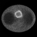
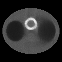
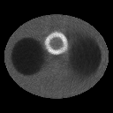
Figure 2: Images reconstructed from the simulated data sets 1(top row) and 2(bottom row) by the classic EM algorithm(left column) and the mean images of 100 trials(right column).

We illustrated four numerical experiments for the proposed algorithms. The first and second experiments are about the projection data set 1(60 projections, 500K) and projection data set 2(30 projections, 100K) to validate the performance of the algorithms for different counts level. The third experiment uses the randomly initial image to test the robustness of the proposed algorithms. In the fourth experiment, we relax the condition of the TV-superiorized EM algorithms 1 and 2 further.
In order to evaluate the qualities of the reconstructed images, we computed the mean images $x^{\ast}$ from 100 noise trials as the standard images of the two data sets, respectively.

$$x^{\ast}={1\over 100}\sum_{m=1}^{100}\hat{x}^{m},$$ (43)

where $\hat{x}^{m}(m=1,2,\cdots,100)$ is the reconstructed image of the $m$th trial by the classic EM algorithm, and the number of iterations for each trial is 30.
As shown in figure 2, the mean images for the two data sets are clear visually, while those reconstructed by the classic EM algorithm are dominated by noise, especially the image for data set 2 due to the low count level. Thus, we use the mean square error (MSE) between the estimation $x$ and the mean image $x^{\ast}$ from the same data set to measure the image qualities, where the MSE is computed by

$$\text{MSE}(x)=\frac{1}{N}\sum_{j=1}^{N}(x_{j}-x_{j}^{\ast})^{2}.$$ (44)

The outputs of the different algorithms were taken as the best estimations in terms of MSE. In order to compare the qualities of images reconstructed from different data sets, we introduced the relative MSE(RMSE) defined as

$$\text{RMSE}(x)=\sqrt{\frac{\sum_{j=1}^{N}(x_{j}-x_{j}^{\ast})^{2}}{\sum^{N}_{j=1}(x^{\ast}_{j})^{2}}},$$ (45)

In the numerical experiments, an uniformly initial image $x^{0}$ of value $c={1\over N}\sum_{i=1}^{M}b_{i}$ was used for all experiments, unless there was a further explanation. The parameters $\beta_{0}$ were chosen as $c/2$ and $c/10$ for the TV- and $l^{1}$-superiorized EM algorithms, respectively. The thresholding $Q_{1}$ and the parameter $\gamma$ were chosen as $0.01$ and $1/2$, respectively. In the following, we use TV-, hard- and soft-alg $n$($n=1,2$) as the abbreviations of the TV-, hard- and soft-superiorized EM algorithm $n$($n=1,2$) for simplicity.
Experiment 1: sixty projections and 500K counts

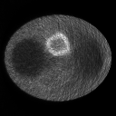
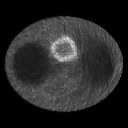
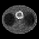
Figure 3: Reconstructed images of experiment 1. The images in top and bottom rows are reconstructed by the superiorized EM algorithms 1 and 2, respectively. The images reconstructed by TV-, hard- and soft-superiorized EM algorithms are displayed from column 1 to column 3.

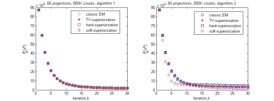
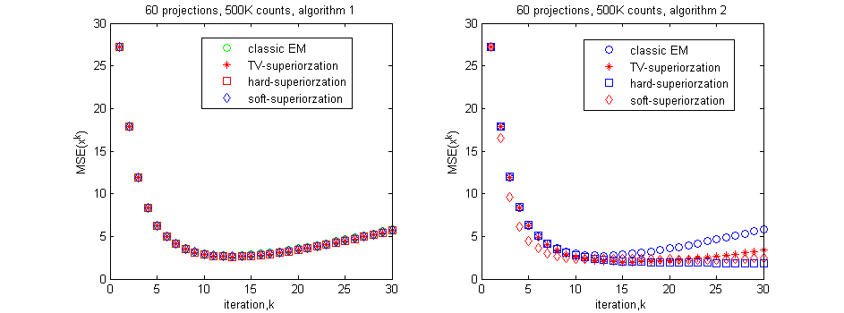
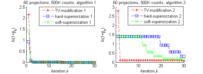
Figure 4: Evolutions of $I_{A}^{b}(x^{k})$(top row), MSE$(x^{k})$(middle row) and $\ln(1+\beta_{k})$(bottom row) of experiment 1.

Table 1: TV values, $l^{1}$-norms, RMSEs and iterations of the reconstructed images of experiment 1.

	EM	TV-alg 1	hard-alg 1	soft-alg 1
TV($\times 10^{3}$)	26.708	25.318	25.577	25.958
$l^{1}$($\times 10^{3}$)	12.953	12.404	12.320	12.489
RMSE	0.1914	0.1873	0.1875	0.1888
iteration	13	13	13	13
	mean	TV-alg 2	hard-alg 2	soft-alg 2
TV($\times 10^{3}$)	13.987	19.434	14.115	15.443
$l^{1}$($\times 10^{3}$)	8.5244	10.279	2.867	3.189
RMSE	-	0.1633	0.1563	0.1747
iteration	-	15	30	23

As expected, the images by the superiorized EM algorithms are superior to the one by the classic EM algorithm in terms of TV value, $l^{1}$-norm and RMSE (see figure 3 and table 1), though the images by the superiorized algorithm 1 are visually indistinguishable from the one by the classic EM algorithm. Furthermore, the superiorized EM algorithm 2 are superior to the superiorized EM algorithm 1, because the regularization parameter $\beta_{k}$ goes to zero very fast for the superiorized EM algorithm 1.
As figure 4 shown, the evolutions of $I_{A}^{b}(x^{k})$ and MSE$(x^{k})$ of the superiorized EM algorithms 1 validate the conclusions of theorem 2.3. Furthermore, the evolutions of $I_{A}^{b}(x^{k})$ and MSE$(x^{k})$ of show the convergence of the superiorized EM algorithms 2, although we can not prove it theoretically. Because the inequality of condition 3 is very strict, the parameters $\beta_{k}$ went to zero very fast for the superiorized algorithm 1. This results in the reconstructed images and the evolutions of $I_{A}^{b}(x^{k})$ and MSE$(x^{k})$ of the superiorized EM algorithms 1 and the classic EM algorithm are indistinguishable from each other, i.e. the regularization of the superiorized EM algorithm 1 is not remarkable.
Although the number of iterations of the superiorized EM algorithm 2 is larger than the classic EM and the superiorized EM algorithm 1(table 1), the superiorized algorithm 2 is superior to the superiorized algorithm 1 in terms of RMSE: RMSE$(x^{tv,13})=0.1668$, RMSE$(x^{h,13})=0.1741$ and RMSE$(x^{s,13})=0.1797$, where $x^{tv,13},x^{h,13},x^{s,13}$ denote the results of tv-, hard- and soft-superiorized algorithms 2, respectively.
Experiment 2: thirty projections and 100K counts

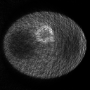
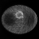
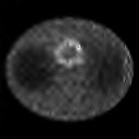
Figure 5: Reconstructed images of experiment 2. The images reconstructed by the TV-, hard- and soft-superiorized EM algorithms 1 and 2 are displayed in columns 2, 3 and 4, and rows 1 and 2, respectively.

Table 2: TV, $l^{1}$-norm, RMSE and iterations of the images of experiment 2.

	EM	TV-alg 1	hard-alg 1	soft-alg 1
TV($\times 10^{3}$)	13.739	13.105	13.396	13.061
$l^{1}$($\times 10^{3}$)	6.729	6.452	6.451	6.277
RMSE	0.2822	0.2778	0.2802	0.2795
iteration	8	8	8	8
	mean	TV-alg 2	hard-alg 2	soft-alg 2
TV($\times 10^{3}$)	7.167	9.769	5.733	5.576
$l^{1}$($\times 10^{3}$)	4.037	5.069	1.434	1.283
RMSE	0	0.2490	0.2091	0.2064
Iteration		9	12	10

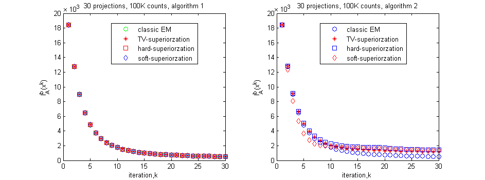
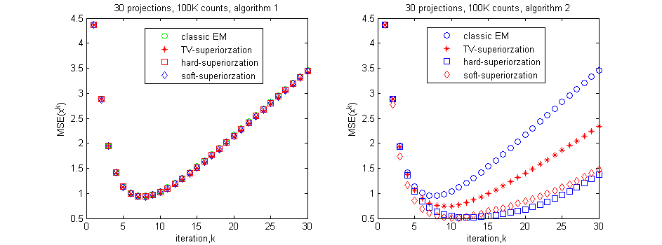
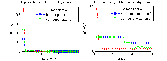
Figure 6: Evolutions of experiment 2. The evolutions of $I_{A}^{b}(x^{k})$(top row), MSE$(x^{k})$(middle row) and $\ln(1+\beta_{k})$(bottom row) of different algorithms.

From the observations of figures 5 and 6, and table 2, we can draw the same conclusions as the experiment 1. Comparing figures 3 and 5, we can see that the visual quality of the images reconstructed from data set 2 are inferior to those reconstructed from data set 1 because of the low count level. And the performance of the superiorized EM algorithms 2 are much more remarkable than the superiorized EM algorithms 1 for data set 2.
Comparing the results of the two experiments above, we can observe that the TV-superiorized EM algorithm 2 is better in terms of RMSE, while the $l^{1}$-superiorized EM algorithms 2 in terms of TV and $l^{1}$-norm values. In addition, the thresholding operations cause the Gibbs oscillations in the reconstructed images by $l^{1}$-superiorized EM algorithms 2.
Because the detectors rotated from top to bottom through left side, the gamma rays emitted from the right part pixels are more likely to be absorbed. Therefore, the right part of the reconstructed images are blurred strongly(see figures 2, 3 and 5).
Experiment 3: initial image $x^{0}$ with random values on interval $[1,2]$ for data set 1
In this experiment, an initial image $x^{0}$ with random values on interval $[1,2]$ and the projection data set 1 are used. The reconstructed images by different algorithms are displayed in figure 7, and the corresponding TV values, $l^{1}$-norms and RMSEs are tabulated in table 3. Because the evolutions of $I_{A}^{b}(x^{k})$ and MSE$(x^{k})$ are very similar to these of experiment 1, we only plot the evolution of $\ln(1+\beta_{k})$ in figure 8.
This experiment shows that the superiorized EM algorithms 2 are stable and robust for initial image. By comparing figures 3 and 7, and tables 1 and 3, we have that the effect of initial image is very strong to the classic EM algorithm and the superiorized EM algorithm 1, but very weak to the superiorized EM algorithm 2.
A surprising observation is that the randomly initial image is superior to the uniformly initial image for the superiorized EM algorithms 2 in term of RMSE by comparing table 1 and table 3. This changes the long-standing opinion about the selection of the initial image for EM-like algorithm, and present a new method to improve the qualities of the reconstructed image.

Table 3: TV values, $l^{1}$-norms, RMSEs and iterations of the images of experiment 3.

	EM	TV-alg 1	hard-alg 1	soft-alg 1
TV($\times 10^{3}$)	40.591	29.804	40.364	34.214
$l^{1}$($\times 10^{3}$)	19.098	14.632	18.907	16.138
RMSE	0.2538	0.2112	0.2529	0.2266
iteration	13	13	13	13
	-	TV-alg 2	hard-alg 2	soft-alg 2
TV($\times 10^{3}$)	-	17.133	16.203	16.372
$l^{1}$($\times 10^{3}$)	-	9.403	3.417	3.207
RMSE	-	0.1469	0.1683	0.1873
Iteration	-	19	30	23

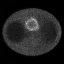
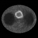
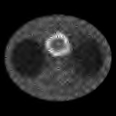
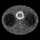
Figure 7: Images of experiment 3. The top image is reconstructed by the classic EM algorithm. The images in columns 1, 2 and 3 and the middle and bottom rows are reconstructed by the TV-, hard- and soft-superiorized EM algorithms 1 and 2, respectively.

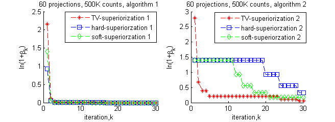
Figure 8: Evolutions of $\ln(1+\beta_{k})$ of experiment 3.

Comparing the evolutions of $\ln(1+\beta_{k})$ in figures 4, 6 and 8, we can observe the following facts. Firstly, the parameter $\beta_{k}$ for the superiorized EM algorithms 1 go to zero fast because of the strict condition 3 of theorem 2.3. Secondly, the reconstructed images of uniformly initial image is more smooth than these of randomly initial image by the TV-superiorized algorithm at low iterations, which results in the parameter $\beta_{k}$ decrease at fast and low rates for experiments 1 and 3, respectively, because of the decreasing condition of the TV function in the conditions ($\ast$) and ($\star$). Thirdly, the thresholding operations(hard and soft) always reduce the $l^{1}$-norm, which implies that the conditions ($\ast$) and ($\star$) for the $l^{1}$-superiorized algorithm 1 and 2 become one condition about the decreasing of K-L distance.
The last observation enlightens us to modify the TV-superiorized EM algorithm further, which discards the deceasing condition of TV function in the conditions ($\ast$) and ($\star$).
Experiment 4: modification of the TV-superiorized algorithms 1 and 2
Figure 9 displays the reconstructed images by the modified versions of TV-superiorized EM algorithms 1 and 2 in absence of the decreasing condition of TV function. The TV values, $l^{1}$-norms, RMSEs and iterations are tabulated in table 4. And figure 10 plots the evolutions of $\ln(1+\beta_{k})$.
As our expectation, the evolution of parameter $\beta_{k}$ of the modified version of TV-superiorized algorithm 2 is similar to the $l^{1}$-superiorized EM algorithm 2, decreasing at much slower rate. However, this modification has very little effect on the TV-superiorized algorithm 1.
It is amazing that the modified algorithms also reduce the TV function (see table 3), even the reconstructed images are better than those reconstructed by the TV-superiorized EM algorithm 2, although we do not validate the decreasing condition of it. The reasons include two aspects. In superiorized algorithms 1 and 2, there are two conditions to control the decreasing of $\beta_{k}$, which causes the size of $\beta_{k}$ is very small at large iterations. Therefore, the strength of regularization is very weak, and the reconstructed image is not good enough. For the modified superiorization algorithms, there is only one condition to control the decreasing of $\beta_{k}$, and $\beta_{k}$ decreases at a lower rate. Therefore, the modified superiorization algorithms can maintain stronger regularization at large iterations, and the reconstructed image is much better. The further study about this algorithm is future work.

Table 4: TV values, $l^{1}$-norm, RMSEs and iterations of the images of experiment 4.

	image 1	image 2	image 3	image 4
TV($\times 10^{3}$)	25.318	12.931	12.955	7.080
$l^{1}$($\times 10^{3}$)	12.404	6.408	7.013	3.399
RMSE	0.1873	0.2772	0.1231	0.1999
iteration	13	8	29	18

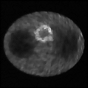
Figure 9: Images of experiment 4. The images in left and right columns are reconstructed from data sets 1 and 2, while the images in first and second rows are reconstructed by modified versions of TV-superiorized EM algorithms 1 and 2, respectively. From left to right and from top to bottom, the images are labeled as image 1 to image 4 for reference.

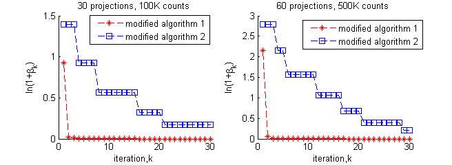
Figure 10: Evolutions of $\ln(1+\beta_{k})$ of experiment 4. Left for data set 1 and right for data set 2, respectively.

Remark 4.1

The experiments show that the superiorized EM algorithm 2 is convergent, though we cannot prove it theoretically so far.

Remark 4.2

The parameter $\beta_{k}$ represents the strength of regularization in a sense, so we can obtain the regularization reconstruction by terminating the algorithms as long as $\beta_{k}$ is smaller than a predefined threshold. As explanation above, the size of $\beta_{k}$ represents the strength of regularization. Therefore, the threshold should be related to the noise level. Intuitively, in order to maintain the regularization strength, the higher the noise level is, the larger the threshold is. The further discussion about the selection of it will be studied in future work.

5 Conclusions and Discussions

In this paper, the convergence of the EM algorithm in the presence of perturbations is discussed, and the superiorized EM algorithm based on the convergent conditions and its modified version are proposed. The numerical experiments validate the correction of theorem 2.3. The superiorized EM algorithms could efficiently reduce the corresponding objective functions which we are superiorizing. Furthermore, The proposed algorithms are more stable and robust than the classic EM algorithm for low counts projection data and randomly initial image.
Although the numerical experiments show the convergence of algorithm 2, we cannot prove the convergence of it theoretically. A more challenging work is about the amazing observation of the experiment 4, which enlightens us to modify the superiorized EM algorithm further. In addition, we could not prove $\phi(x^{\ast})\leq\phi(\hat{x})$ theoretically, where $\hat{x}$ and $x^{\ast}$ are the solutions by the classic iteration algorithm and the $\phi$-superiorization version [25].

References

- [1] M. N. Wernick and J. N. Aarsvold, Emission Tomography: the Fundamentals of PET and SPECT. California: Elsevier Acdamic Press, 2004.
- [2] G. T. Herman, Image Reconstruction from Projection: the Fundamentals of Computerized Tomography. New York: Academic Press, 1980.
- [3] F. Natterer and F. Wübbeling, Mathematical Methods in Image Reconstruction. Philadelphia: Society for Industrial and Applied Mathematics, 2001.
- [4] O. Tretiak and C. Metz, “The exponential Radon transform,” SIAM Journal on Applied Mathematics, vol. 39, no. 2, pp. 341–354, 1980.
- [5] F. Natterer, “Inversion of the attenuated Radon transform,” Inverse Problems, vol. 17, no. 1, pp. 113–119, 2001.
- [6] R. G. Novikov, “An inversion formula for the attenuated X-ray transformation,” Arkiv för Matematik, vol. 40, no. 1, pp. 145–167, 2002.
- [7] F. Noo and J.-M. Wagner, “Image reconstruction in 2D SPECT with 180∘ acquisition,” Inverse Problems, vol. 17, no. 5, pp. 1357–1371, 2001.
- [8] F. Noo, M. Defrise, J. D. Pack, and R. Clackdoyle, “Image reconstruction from truncated data in single-photon emission computed tomography with uniform attenuation,” Inverse Problems, vol. 23, no. 2, pp. 645–667, 2007.
- [9] L. A. Shepp and Y. Vardi, “Maximum likelihood restoration for emission tomography,” IEEE Transactions on Medical Imaging, vol. 1, no. 2, pp. 113–122, 1982.
- [10] H. M. Hudson and R. S. Larkin, “Accelerated image reconstruction using ordered subsets of projection data,” IEEE Transactions on Medical Imaging, vol. 13, no. 4, pp. 601–609, 1994.
- [11] I. Hsiao and H. Huang, “An accelerated ordered subsets reconstruction algorithm using an accelerating power factor for emission tomography,” Physics in Medicine and Biology, vol. 55, no. 3, pp. 599–614, 2010.
- [12] Y. Vardi, L. A. Shepp, and L. Kaufman, “A statistical model for positron emission tomography,” Journal of the American Statistical Association, vol. 80, no. 389, pp. 8–20, 1985.
- [13] R. Gordon, R. Bender, and G. T. Herman, “Algebraic reconstruction techniques (ART) for three-dimensional electron microscopy and X-ray photography,” Journal of Theoretical Biology, vol. 29, no. 3, pp. 471–482.
- [14] Y. Censor, T. Elfving, and G. T. Herman, “Averaging strings of sequential iterations for convex feasibility problems,” in Inherently Parallel Algorithms in Feasibility and Optimization and their Applications, pp. 101–113, 2001.
- [15] E. Y. Sidky, C.-M. Kao, and X. Pan, “Accurate image reconstruction from few-views and limited-angle data in divergent-beam CT,” X-Ray Science and Technology, vol. 14, pp. 119–139, 2006.
- [16] S. J. LaRoque, E. Y. Sidky, and X. Pan, “Accurate image reconstruction from few-view and limited-angle data in diffraction tomography,” Journal of the Optical Society of America, vol. 25, no. 7, pp. 1772–1782, 2008.
- [17] X. Pan, E. Y. Sidky, and M. Vannier, “Why do commercial CT scanners still employ traditional, filtered backprojection for image reconstruction?,” 2009.
- [18] M. Defrise, C. Vanhove, and X. Liu, “An algorithm for total variation regularization in high-dimensional linear problems,” Inverse Problems, vol. 27, no. 6, p. 065002, 2011.
- [19] E. Y. Sidky, J. H. Jøgensen, and X. Pan, “Convex optimization problem prototyping for image reconstruction in computed tomography with the Chambolle-Pock algorithm,” Physics in Medicine and Biology, vol. 57, no. 10, pp. 3065–3091, 2012.
- [20] B. Dong, J. Li, and Z. Shen, “X-ray CT image reconstruction via wavelet frame based regularization and Radon domain inpainting,” Journal of Scientific Computing, vol. 54, no. 2-3, pp. 333–349, 2013.
- [21] D. Butnariu, R. Davidi, G. T. Herman, and I. G. Kazantsev, “Stable convergence behavior under summable perturbations of a class of projection methods for convex feasibility and optimization problem,” IEEE Journal of Selected Topics Signal Processing, vol. 1, no. 4, pp. 540–547, 2007.
- [22] G. T. Herman and R. Davidi, “Image reconstruction from a small number of projections,” Inverse Problems, vol. 24, no. 4, p. 045011, 2008.
- [23] E. Garduo, G. T. Herman, and R. Davidi, “Reconstruction from a few projections by minimization of the Haar transform,” Inverse Problems, vol. 24, no. 4, p. 0550061, 2011.
- [24] A. Chambolle and T. Pock, “A first-order primal-dual algorithm for convex problem with apllications to imaging,” Journal of Mathematical Imaging and Vision, vol. 40, no. 1, pp. 120–145, 2011.
- [25] Y. Censor, R. Davidi, and G. T. Herman, “Perturbation resilience and superiorization of iteration algorithm,” Inverse Problems, vol. 26, no. 6, p. 065008, 2010.
- [26] R. Davidi, G. T. Herman, and Y. Censor, “Perturbation-resilient block-iterative projection methods with application to image reconstruction from projection,” International Transactions in Operational Research, vol. 16, no. 2, pp. 505–524, 2009.
- [27] T. Nikazad, R. Davidi, and G. T. Herman, “Accelerated perturbation-resilient block-iterative projection methods with application to image reconstruction,” Inverse Problems, vol. 28, no. 3, p. 035005, 2012.
- [28] W. Jin, Y. Censor, and M. Jiang, “A heuristic superiorization-like approach to bioluminescence tomography,” in Proceedings of the International Federation for Medical and Biological Engineering (IFMBE), vol. 39, Springer-Verlag, 2012.
- [29] L. I. Rudin, S. Osher, and E. Fatemi, “Nonlinear total variation based noise removal algorithms,” Physca D., vol. 60, no. 1, pp. 259–268, 1992.
- [30] E. Candes, J. Romberg, and T. Tao, “The dantzig selector: Statistical estimation when is much larger than ,” the Annals of Statistics, vol. 35, no. 6, pp. 2313–2351, 2007.
- [31] D. L. Snyder, T. J. Schulz, and J. A. O. Sullivan, “Deblurring subject to nonnegativity constraints,” IEEE Transactions on Signal Processing, vol. 40, no. 5, pp. 1143–1150, 1992.
- [32] E. Candes, J. Romberg, and T. Tao, “Robust uncertainty principles: Exact signal reconstruction from highly incomplete frequency information,” IEEE Transactions on Information Theory, vol. 52, no. 2, pp. 489–509, 2006.
- [33] H. Yu and G. Wang, “Compressed sensing based interior tomography,” Physics in Medicine and Biology, vol. 54, no. 9, pp. 2791–2805, 2009.
- [34] J. A. fessler, “Matlab code for emission tomography.” http://www.eecs.umich.edu/ fessler/.