Variational integrators for underactuated mechanical control systems with symmetries

Abstract.

Optimal control problems for underactuated mechanical systems can be seen as a higher-order variational problem subject to higher-order constraints (that is, when the Lagrangian function and the constraints depend on higher-order derivatives such as the acceleration, jerk or jounces). In this paper we discuss the variational formalism for the class of underactuated mechanical control systems when the configuration space is a trivial principal bundle and the construction of variational integrators for such mechanical control systems.

An interesting family of geometric integrators can be defined using discretizations of the Hamilton’s principle of critical action. This family of geometric integrators is called variational integrators, being one of their main properties the preservation of geometric features as the symplecticity, momentum preservation and good behavior of the energy. We construct variational integrators for higher-order mechanical systems on trivial principal bundles and their extension for higher-order constrained systems and we devote special attention to the particular case of underactuated mechanical systems

1. Introduction

The construction of variational integrators have received a lot of interest in the recent years from the theoretical and applied points of view. The goal of this paper is to develop variational integrators for optimal control problems of mechanical systems defined on a trivial principal bundle, paying particular attention to underactuated mechanical control systems. Underactuated control systems are characterized by the fact that they have more degrees of freedom than actuators.

The presence of underactuated mechanical systems is ubiquitous in engineering applications; for instance, the underactuation may arise from a failure in the fully actuated regime or in the design of less costly devices. Optimal control problems of underactuated mechanical systems can be seen as a variational problem involving Lagrangians defined on higher-order tangent bundles subject to higher-order constraints. That is, Lagrangian and constraint functions depending not just on positions and velocities, but also on acceleration and sometimes higher-order derivatives of the curve in the configuration space. The purpose of the optimal control problem is to find a curve of the state variables and control inputs which satisfies the controlled equations and minimizes a cost function subject to initial and final boundary conditions. We will use the equivalence between optimal control problems of underactuated mechanical systems and second-order variational problems with second-order constraints (see [3]) when the configuration manifold is a trivial principal bundle. To develop this process it is necessary to obtain the second-order Euler-Lagrange equations, calculation which is showed in great detail. Furthermore, the Lagrange-Poincaré equations follow from the Euler-Lagrange ones after applying a symmetry reduction procedure. Moreover, recent developments in the theory of $k-$splines on $SO(3)$ and the Clebsh-Pontryagin optimal control problem (see [19, 20]), suggest that the higher-order situation may be relevant. Consequently, we extend the previous calculation to this case, obtaining Lagrange-Poincaré equations using a left trivialization of the tangent bundle of a Lie group.

Higher-order variational problems also have been used in the applications to longitudinal studies in computational anatomy. This kind of studies seeks, among other goals, to determine a path that interpolates optimally through a time-order series of images or shapes. Depending on the specific application, the interpolant will be require to have a certain degree of spatiotemporal smoothness. If a higher-order degree of smoothness is required, a natural approach is to investigate higher-order variational formulation of the interpolation problem (see for example [8],[10], [20] and [39]).

In order to obtain variational integrators for the systems described above, we extend the theory of discrete mechanics, which is based on discrete calculus of variations, to higher-order systems subject to higher-order constraints. The discrete approach proposed in this work (we will employ our setting or our approach henceforth for sake of simplicity) follows the ideas proposed by Marsden and Wendlandt [37] and Marsden and West [38] for first order systems without constraints. In particular, we shall develop the discrete analogue of higher-order Euler-Lagrange and Lagrange-Poincaré equations (introduced by Gay-Balmaz, Holm and Ratiu in [18]) for trivial principal bundles and its extension to constrained systems. With this particular purpose, we use the discrete Hamilton’s principle and the adding of Lagrange multipliers in order to obtain discrete paths that approximately satisfy the dynamics and the constraints. Such formulation gives us the preservation of important geometric properties of the mechanical system, such as momentum, symplecticity, group structure and good behavior of the energy (see [21]). The preservation of these geometric properties produces an improved qualitative behavior, and also a more accurate long-time integration than with a standard integrator.

The methods studied in this paper are founded on recently developed structure-preserving numeric integrators for optimal control problems (see [3, 8, 13, 14, 15, 25, 27, 28, 31, 35, 40] and references therein) based on solving a discrete optimal control problem as a discrete variational problem with constraints (see [3, 14, 15] for the continuous counterpart). These numerical integrators are used for simulating and controlling the dynamics of satellites, spacecrafts, underwater vehicles, mobile robots, helicopters and wheeled vehicles [4, 9, 30]. More concretely, previous results (upon which the present ones are based) can be found in [13] and [24], where mainly the treated configuration manifolds are Lie groups and in the second work the authors solve optimal control problems with a different view point, where they construct variational integrators for systems with piecewise controls. Previous numerical methods are developed only for the case of higher-order tangent bundles [15],[16] or several copies of the Lie algebra of a Lie group (see for example [8], [13]). Both correspond to numerical methods for higher-order Euler-Lagrange equations and Euler-Poincaré equations, respectively. However, real systems are typically modeled over a manifold which admits a Lie group of symmetries (mainly $SE(2)$, $SO(2)$, $SE(2)$ and $SE(3)$). Therefore, applying standard reduction theory we derive a system defined on a quotient bundle. This bundle is, in several cases, the cartesian product of the previously mentioned spaces; that is, a higher-order tangent bundle and several copies of a Lie algebra associated with the symmetry Lie group. Thus we design geometric integrators for this type of spaces, which includes the previous ones as particular cases, and we apply this construction to the desing of variational integrator for optimal control problems of mechanical systems in presence of Lie groups symmetries (see [5],[6], [16], [15]).

To be self-contained, we introduce a brief background in discrete mechanics.

1.1. General Background

A discrete Lagrangian is a map $L_{d}\colon Q\times Q\to\mathds{R}$, which may be considered as an approximation of the integral action defined by a continuous Lagrangian $L\colon TQ\to\mathds{R},$

$$L_{d}(q_{0},q_{1})\approx\int^{h}_{0}L(q(t),\dot{q}(t))\;dt,$$

where $q(t)$ is the unique solution of the Euler-Lagrange equations for $L$; $q(0)=q_{0}$, $q(h)=q_{1}$ and the time step $h>0$ is small enough.

Given the grid $\{t_{k}=kh\mid k=0,\ldots,N\}$, with $Nh=T$, define the discrete path space $\mathcal{C}_{d}(Q):=\{q_{d}:\{t_{k}\}_{k=0}^{N}\rightarrow Q\}.$ This discrete path space is isomorphic to the smooth product manifold which consists of $N+1$ copies of $Q$. The discrete trajectory $q_{d}\in\mathcal{C}_{d}(Q)$ will be identified with its image $q_{d}=\{q_{k}\}_{k=0}^{N}$ where $q_{k}:=q_{d}(t_{k}).$

Define the action sum $\mathcal{A}_{d}\colon\mathcal{C}_{d}(Q)\to\mathds{R}$, associated to $L_{d}$, by summing the discrete Lagrangian on each adjacent pair

$${\mathcal{A}_{d}}(q_{d}):=\sum_{k=1}^{N-1}L_{d}(q_{k-1},q_{k}),$$

where $q_{k}\in Q$ for $0\leq k\leq N.$ Note that the discrete action inherits the smoothness of the discrete Lagrangian.

The discrete variational principle then requires that $\delta{\mathcal{A}_{d}}=0$ where the variations are taken with respect to each point $q_{k},$ $1\leq k\leq N-1$ along the path, and the resulting equations of motion (a system of difference equations), given fixed endpoints $q_{0}$ and $q_{N},$ are

$$D_{1}L_{d}(q_{k},q_{k+1})+D_{2}L_{d}(q_{k-1},q_{k})=0,$$ (1)

where $D_{1}$ and $D_{2}$ denote the derivative of the discrete Lagrangian with respect to the first and second arguments, respectively. These equations are usually called discrete Euler–Lagrange equations.

If the matrix $D_{12}L_{d}(q_{k},q_{k+1})$ is regular, it is possible to define a (local) discrete flow $\Upsilon_{L_{d}}\colon Q\times Q\to Q\times Q$, by $\Upsilon_{L_{d}}(q_{k-1},q_{k})=(q_{k},q_{k+1})$ from (1). This discrete flow preserves the (pre-)symplectic form on $Q\times Q,$ $\omega_{d}$, i.e. $\Upsilon_{L_{d}}^{*}\omega_{d}=\omega_{d}$ (see [37], [38] and references therein).

Given an action of a Lie group $G$ on $Q$, we can consider the $G-$action on $Q\times Q$ $g\cdot(q_{k},q_{k+1}):=(g\cdot q_{k},g\cdot q_{k+1})$. Denoting by $\mathfrak{g}$ the Lie algebra of $G$ we can define two discrete momentum maps

$$J_{d}^{\pm}(q_{k},q_{k+1}): \mathfrak{g}\rightarrow\mathds{R}$$

$$\xi\mapsto\langle\Theta_{L_{d}}^{\pm}(q_{k},q_{k+1}),\xi_{Q\times Q}(q_{k},q_{k+1})\rangle$$

for $\xi\in\mathfrak{g}.$ Here $\xi_{Q\times Q}(q_{k},q_{k+1}):=(\xi_{Q}(q_{k}),\xi_{Q}(q_{k+1}))$ where

$$\xi_{Q}(q)=\frac{d}{dt}\Big{|}_{t=0}(exp(t\xi)\cdot q)$$

denotes the fundamental vector field and $\Theta^{+}_{L_{d}}(q_{k},q_{k+1}):=D_{2}L_{d}(q_{k},q_{k+1})dq_{k+1},$ $\Theta^{-}_{L_{d}}(q_{k},q_{k+1}):=-D_{1}L_{d}(q_{k},q_{k+1})dq_{k}$ are the discrete Poincaré-Cartan 1-forms on $Q\times Q.$ If the Lagrangian is $G-$invariant then $J_{d}:=J_{d}^{+}=J_{d}^{-}$ and $J_{d}\circ\Upsilon_{d}=J_{d}.$

1.2. Goals, contributions and organization of the paper.

The main goal of this work is to develop variational integrators for optimal control problems of underactuated mechanical systems defined on a trivial principal bundle. This is achieved in section §5, where the process is showed in great detail for two examples. With that purpose, other contributions are presented previously. Namely: in §2 the continuous Euler-Lagrange (Lagrange-Poincaré) equations for higher-order tangent bundles when the configuration manifold is a trivial principal bundle are obtained, particularly in theorem 2.2; section §3 is devoted to the construction of variational integrators for higher-order mechanical systems with symmetries where we obtain the discrete higher-order Euler-Lagrange and Lagrange-Poincaré equations in theorem 3.2; in §4 higher-order constraints are added into the picture and consequently we obtain the equations of motion for constrained system, both in the continuous and discrete cases by using Lagrange multipliers; and, finally, in §5 we study optimal control problems, we apply the techniques developed previously in order to obtain the design of geometric numerical integrators for this kind of optimal control problems and explore two examples: the optimal control of a vehicle whose configuration space is the Lie group $SE(2),$ and the associated optimal control problem of a homogeneous ball rotating on a plate.

2. Higher-order Euler-Lagrange equations on trivial principal bundles

2.1. Higher-order tangent bundles

In this subsection we recall some basic facts of the higher-order tangent bundle theory. At some point, we will particularize this construction to the case when the configuration space is a Lie group $G$. For more details see [32].

Let $M$ be a differentiable manifold of dimension $n$. It is possible to introduce an equivalence relation in the set $C^{l}(\mathds{R},M)$ of $l$-differentiable curves from $\mathds{R}$ to $M$. By definition, two given curves in $M$, $\gamma_{1}(t)$ and $\gamma_{2}(t)$, where $t\in(-a,a)$ with $a\in\mathds{R}$ have contact of order $l$ at $q_{0}=\gamma_{1}(0)=\gamma_{2}(0)$ if there is a local chart $(\varphi,U)$ of $M$ such that $q_{0}\in U$ and

$$\frac{d^{s}}{dt^{s}}\left(\varphi\circ\gamma_{1}(t)\right){\Big{|}}_{t=0}=\frac{d^{s}}{dt^{s}}\left(\varphi\circ\gamma_{2}(t)\right){\Big{|}}_{t=0}\;,$$

for all $s=0,...,l.$ This is a well-defined equivalence relation in $C^{l}(\mathds{R},M)$ and the equivalence class of a curve $\gamma$ will be denoted by $[\gamma]_{0}^{(l)}.$ The set of equivalence classes will be denoted by $T^{(l)}M$ and it is not hard to show that it has a natural structure of differentiable manifold. Moreover, $\tau_{M}^{l}:T^{(l)}M\rightarrow M$ where $\tau_{M}^{l}\left([\gamma]_{0}^{(l)}\right)=\gamma(0)$ is a fiber bundle called the tangent bundle of order $l$ of $M.$

Define the left- and right-translation of $G$ on itself

$$\ell:G\times G \to G\,,\qquad\;(g,h)\,\mapsto\ell_{g}(h)=gh,$$

$$r:G\times G \to G\,,\qquad\;(g,h)\,\mapsto r_{g}(h)=hg.$$

Obviously $\ell_{g}$ and $r_{g}$ are diffeomorphisms.

The left-translation allows us to trivialize the tangent bundle $TG$ and the cotangent bundle $T^{*}G$ as follows

$$TG \to G\times{\mathfrak{g}},\qquad\,\,(g,\dot{g})\,\,\,\longmapsto(g,g^{-1}\dot{g})=(g,T_{e}\ell_{g^{-1}}\dot{g})=(g,\xi),$$

$$T^{*}G \to G\times{\mathfrak{g}}^{*},\qquad(g,\alpha_{g})\longmapsto(g,T^{*}_{e}\ell_{g}(\alpha_{g}))=(g,\alpha),$$

where ${\mathfrak{g}}=T_{e}G$ is the Lie algebra of $G$ and $e$ is the neutral element of $G$. In the same way, we have the identification $TTG\equiv G\times 3{\mathfrak{g}}$ where $3\mathfrak{g}$ stands for $\mathfrak{g}\times\mathfrak{g}\times\mathfrak{g}$. Throughout this paper, the notation $n\,V$, where $V$ is a given space, denotes the cartesian product of $n$ copies of $V$. Therefore, in the case when the manifold $M$ has a Lie group structure, i.e. $M=G$, we can use the left trivialization to identify the higher-order tangent bundle $T^{(l)}G$ with $G\times l{\mathfrak{g}}$. That is, if $g:I\rightarrow G$ is a curve in $C^{l}(\mathds{R},G)$, where $I\subset\mathds{R}$, then:

$$\begin{array}[]{rrcl}\Upsilon^{(l)}:&T^{(l)}G&\longrightarrow&G\times l{\mathfrak{g}}\\ &[g]_{0}^{(l)}&\longmapsto&\left(g(0),g^{-1}(0)\dot{g}(0),\frac{d}{dt}\Big{|}_{t=0}(g^{-1}(t)\dot{g}(t)),\ldots,\frac{d^{l-1}}{dt^{l-1}}\Big{|}_{t=0}(g^{-1}(t)\dot{g}(t))\right).\end{array}$$

It is clear that $\Upsilon^{(l)}$ is a diffeomorphism.

We will denote $\xi(t):=g^{-1}(t)\dot{g}(t)$, therefore

$$\Upsilon^{(l)}([g]_{0}^{(l)})=(g,\xi,\dot{\xi},\ldots,\xi^{(l-1)})\;,$$

where

$$\xi^{(j)}(t)=\frac{d^{j}}{dt^{j}}(g^{-1}(t)\dot{g}(t)),\qquad 0\leq j\leq l-1$$

and $g(0)=g,\xi^{(j)}(0)=\xi^{(j)},0\leq j\leq l-1$. We will use the following notations without distinction $\xi^{(0)}=\xi$, $\xi^{(1)}=\dot{\xi}$, $\xi^{(2)}=\ddot{\xi}$ and so on, when referring to the derivatives.

We may also define the surjective mappings $\tau_{G}^{(j,l)}:T^{(l)}G\rightarrow T^{(j)}G,$ for $j\leq l$, given by $\tau_{G}^{(j,l)}\left([g]_{0}^{(l)}\right)=[g]_{0}^{(j)}.$ With the previous identifications we have that

$$\tau_{G}^{(j,l)}(g(0),\xi(0),\dot{\xi}(0),\ldots,\xi^{(l-1)}(0))=(g(0),\xi(0),\dot{\xi}(0),\ldots,\xi^{(j-1)}(0)).$$

It is easy to see that $T^{(1)}G\equiv G\times{\mathfrak{g}}$, $T^{(0)}G\equiv G$ and $\tau_{G}^{(0,l)}=\tau_{G}^{l}$.

2.2. Euler-Lagrange equations for trivial principal bundles

In this subsection and the two subsequent ones we derive, from a variational point of view, the Euler-Lagrange equations for the trivial principal bundle $M=Q\times G$ where $Q$ is a $n-$dimensional differentiable manifold and $G$ is a Lie group. We consider the cases of the tangent bundle (see [11] for more details), second-order tangent bundle and higher-order tangent bundle where we show the process step by step since it may be enlightening for the reader.

Let $L:TM\rightarrow\mathds{R}$ be a Lagrangian function. Since $TG$ can be identified with $G\times\mathfrak{g}$ after a left-trivialization, we can consider a Lagrangian function as $L:TQ\times G\times\mathfrak{g}\rightarrow\mathds{R}$.

The motion of the mechanical system is described by applying the following variational principle:

$$\delta\mathcal{A}(c):=\delta\int_{0}^{T}L(c(t),\dot{c}(t))dt:=\delta\int_{0}^{T}L(q(t),\dot{q}(t),g(t),\xi(t))dt=0,$$ (2)

where $c$ is a smooth curve on $Q\times G$ and, with some abuse of notation, $\dot{c}(t)\in TQ\times G\times\mathfrak{g}$, which locally reads $\dot{c}(t)=(q(t),\dot{q}(t),g(t),\xi(t))$. The variations $\delta q(t)$ satisfy $\delta q(0)=\delta q(T)=0,$ and $\delta\xi$ verify $\delta\xi(t)=\dot{\eta}(t)+[\xi(t),\eta(t)]=\dot{\eta}(t)+\mbox{ad}_{\xi(t)}\eta(t)$, where $\eta(t)$ is an arbitrary curve on the Lie algebra with $\eta(0)=\eta(T)=0$ given by $\eta=g^{-1}\delta g$ (see [22]). This variational principle gives rise to the Euler-Lagrange equations on trivial principal bundles

$$\frac{d}{dt}\left(\frac{\partial L}{\partial\dot{q}}\right) =\frac{\partial L}{\partial q},$$ (3a)

$$\frac{d}{dt}\left(\frac{\partial L}{\partial\xi}\right) =\hbox{ad}^{*}_{\xi}\left(\frac{\partial L}{\partial\xi}\right)+\ell_{g}^{*}\frac{\partial L}{\partial g},$$ (3b)

where $\hbox{ad}^{*}:\mathfrak{g}^{*}\rightarrow\mathfrak{g}^{*}$ is the coadjoint representation of the Lie algebra $\mathfrak{g}.$ If the Lagrangian $L$ is left-invariant, that is, $L$ does not depend on the variable on $G,$ we can perform a reduction procedure yielding a reduced Lagrangian function $L_{\tiny\mbox{red}}:TQ\times\mathfrak{g}\to\mathds{R}$. Then the above equations are rewritten as

$$\frac{d}{dt}\left(\frac{\partial L_{\tiny\mbox{red}}}{\partial\dot{q}}\right) =\frac{\partial L_{\tiny\mbox{red}}}{\partial q}$$ (4a)

$$\frac{d}{dt}\left(\frac{\partial L_{\tiny\mbox{red}}}{\partial\xi}\right) =\hbox{ad}^{*}_{\xi}\left(\frac{\partial L_{\tiny\mbox{red}}}{\partial\xi}\right),$$ (4b)

which are called Lagrange-Poincaré equations (see [11]).

2.3. Second-order Euler-Lagrange equations for trivial principal bundles

In this subsection we develop from a variational point of view, Euler-Lagrange equations for second-order Lagrangian systems defined in a trivial principal bundle, moreover, when the second-order Lagrangian is $G$-invariant we obtain second-order Lagrange-Poincaré equations. These results also appear in [18] with the motivation of future studies in computational anatomy.

Let $L:T^{(2)}Q\times G\times 2\mathfrak{g}\rightarrow\mathbb{R}$ be a Lagrangian function. The problem consists in finding the critical curves of the action defined by

$$\mathcal{A}(c):=\int_{0}^{T}L(c(t),\dot{c}(t),\ddot{c}(t))dt:=\int_{0}^{T}L(q(t),\dot{q}(t),\ddot{q}(t),g(t),\xi(t),\dot{\xi}(t))dt$$

among all the smooth curves $c$ in $(Q\times G)$ with fixed endpoint conditions. As in the previous subsection we employ the notation $\ddot{c}(t)\in T^{(2)}Q\times G\times 2\mathfrak{g}$ which locally reads $\ddot{c}(t)=(q(t),\dot{q}(t),\ddot{q}(t),g(t),\xi(t),\dot{\xi}(t))$. In order to clarify the procedure of taking variations in a Lie group we introduce here some notation. We shall consider arbitrary variations of the curve $c$, i.e. $\delta c=(\delta q,\delta q^{(1)},\delta q^{(2)},\delta g,\delta\xi,\delta\dot{\xi})$, where $\delta q:=\frac{d}{d\epsilon}|_{{}_{\epsilon=0}}q_{\epsilon}$, $\delta q^{(l)}:=\frac{d^{l}}{dt^{l}}\delta q\,\,(\hbox{ for }l=1,2)$, and $\delta g:=\frac{d}{d\epsilon}|_{{}_{\epsilon=0}}g_{\epsilon}.$ Here $\epsilon\mapsto q_{\epsilon}$ and $\epsilon\mapsto g_{\epsilon}$ are smooth curves on $Q$ and $G$ respectively, for $\epsilon\in(-a,a)\subset\mathds{R}$, such that $q_{0}=q$ and $g_{0}=g.$ For any $\epsilon,$ we define an element of the Lie algebra by $\xi_{\epsilon}:=g^{-1}_{\epsilon}\dot{g}_{\epsilon}.$ Its corresponding variation $\delta\xi$ induced by $\delta g$ is $\delta\xi=\dot{\eta}+[\xi,\eta]$ where $\eta:=g^{-1}\delta g\in\mathfrak{g}$. Therefore

$$\delta\mathcal{A}(c) = \delta\int_{0}^{T}L(q(t),\dot{q}(t),\ddot{q}(t),g(t),\xi(t),\dot{\xi}(t))dt$$

$$= \frac{d}{d\epsilon}\Big{|}_{\epsilon=0}\int_{0}^{T}L(q_{\epsilon}(t),\dot{q}_{\epsilon}(t),\ddot{q}_{\epsilon}(t),g_{\epsilon}(t),\xi_{\epsilon}(t),\dot{\xi}_{\epsilon}(t))dt$$

$$= \int_{0}^{T}\left(\Big{\langle}\frac{\partial L}{\partial\ddot{q}},\frac{d^{2}}{dt^{2}}(\delta q)\Big{\rangle}+\Big{\langle}\frac{\partial L}{\partial\dot{q}},\frac{d}{dt}(\delta q)\Big{\rangle}+\Big{\langle}\frac{\partial L}{\partial q},\delta q\Big{\rangle}\right.$$

$$\left.+\Big{\langle}\frac{\partial L}{\partial g},\delta g\Big{\rangle}+\Big{\langle}\frac{\partial L}{\partial\dot{\xi}},\frac{d}{dt}(\delta\xi)\Big{\rangle}+\Big{\langle}\frac{\partial L}{\partial\xi},\delta\xi\Big{\rangle}\right)dt.$$

Using twice integration by parts and the endpoint conditions $q(0)=q(T)=\dot{q}(0)=\dot{q}(T)=0$ and $\eta(0)=\eta(T)=\dot{\eta}(0)=\dot{\eta}(T)=0,$ the stationary condition $\delta\mathcal{A}(c)=0$ implies

$$0 = \int_{0}^{T}\Big{\langle}\frac{d}{dt}\left(\frac{d}{dt}\frac{\partial L}{\partial\ddot{q}}-\frac{\partial L}{\partial\dot{q}}\right)+\frac{\partial L}{\partial q},\delta q\Big{\rangle}dt$$

$$+\int_{0}^{T}\Big{\langle}\ell_{g}^{*}\left(\frac{\partial L}{\partial g}\right),\eta\Big{\rangle}dt+\int_{0}^{T}\Big{\langle}\left(-\frac{d}{dt}+\mbox{ad}^{*}_{\xi}\right)\left(\frac{\partial L}{\partial\xi}-\frac{d}{dt}\frac{\partial L}{\partial\dot{\xi}}\right),\eta\Big{\rangle}dt$$

Therefore, $\delta\mathcal{A}(c)=0$ if and only if $c\in\mathcal{C}^{\infty}(Q\times G)$ is a solution of the second-order Euler-Lagrange equations for $L:T^{(2)}Q\times G\times 2\mathfrak{g}\rightarrow\mathds{R},$

$$\frac{d}{dt}\left(\frac{\partial L}{\partial\dot{q}}-\frac{d}{dt}\frac{\partial L}{\partial\ddot{q}}\right) =\frac{\partial L}{\partial q},$$ (5a)

$$\left(\frac{d}{dt}-\mbox{ad}^{*}_{\xi}\right)\left(\frac{\partial L}{\partial\xi}-\frac{d}{dt}\frac{\partial L}{\partial\dot{\xi}}\right) =\ell_{g}^{*}\frac{\partial L}{\partial g},$$ (5b)

which split into a $Q$ part (5a) and a $G$ part (5b). The previous development, reaching equations (5), shall be considered as the proof of the following result,

Theorem 2.1.

Let $L:T^{(2)}Q\times G\times 2\mathfrak{g}\rightarrow\mathds{R}$ be a Lagrangian where the left-trivialization $\xi(t):=g^{-1}(t)\dot{g}(t)\in\mathfrak{g}$ has been considered, and $\eta(t)$ is a curve on $\mathfrak{g}$ with fixed endpoints $\eta(0)=\eta(T)=0.$ The curve $c\in\mathcal{C}^{\infty}(Q\times G)$ satisfies $\delta\mathcal{A}(c)=0$ for the action $\mathcal{A}:\mathcal{C}^{\infty}(Q\times G)\rightarrow\mathds{R}$ given by

$$\mathcal{A}(c)=\int_{0}^{T}L(q,\dot{q},\ddot{q},g,\xi,\dot{\xi})dt,$$

with endpoint conditions $\delta q(0)=\delta q(T)=0$ and $\delta\dot{q}(0)=\delta\dot{q}(T)=0$; if and only if $c$ is a solution of the second-order Euler-Lagrange equations for $L$,

$$\frac{\partial L}{\partial q}-\frac{d}{dt}\frac{\partial L}{\partial\dot{q}}+\frac{d^{2}}{dt^{2}}\frac{\partial L}{\partial\ddot{q}} = 0,$$

$$\ell_{g}^{*}\frac{\partial L}{\partial g}+\mbox{\mbox{ad}}^{*}_{\xi}\frac{\partial L}{\partial\xi}-\mbox{ad}^{*}_{\xi}\left(\frac{d}{dt}\frac{\partial L}{\partial\dot{\xi}}\right)-\frac{d}{dt}\frac{\partial L}{\partial\xi}+\frac{d^{2}}{dt^{2}}\frac{\partial L}{\partial\dot{\xi}} = 0.$$

Corollary 2.1.

If the Lagrangian $L:T^{(2)}Q\times G\times 2\mathfrak{g}\to\mathds{R}$ is left-invariant, that is if $L$ does not depend on $g\in G$, we can induce a reduced Lagrangian $L_{\tiny\mbox{red}}:T^{(2)}Q\times 2\mathfrak{g}\to\mathds{R}$ whose equations of motion are

$$\frac{\partial L_{\tiny\mbox{red}}}{\partial q}-\frac{d}{dt}\frac{\partial L_{\tiny\mbox{red}}}{\partial\dot{q}}+\frac{d^{2}}{dt^{2}}\frac{\partial L_{\tiny\mbox{red}}}{\partial\ddot{q}} =0,$$ (6a)

$$\mbox{ad}^{*}_{\xi}\frac{\partial L_{\tiny\mbox{red}}}{\partial\xi}-\mbox{ad}^{*}_{\xi}\left(\frac{d}{dt}\frac{\partial L_{\tiny\mbox{red}}}{\partial\dot{\xi}}\right)-\frac{d}{dt}\frac{\partial L_{\tiny\mbox{red}}}{\partial\xi}+\frac{d^{2}}{dt^{2}}\frac{\partial L_{\tiny\mbox{red}}}{\partial\dot{\xi}} =0.$$ (6b)

These equations are called second-order Lagrange-Poincaré equations.

2.4. Higher-order Euler-Lagrange equations on trivial principal bundles

The previous ideas can be extended to Lagrangians defined on a higher-order trivial principal bundle. We identify the higher-order tangent bundle $T^{(l)}M$, for $l>2$, with $T^{(l)}Q\times G\times l\mathfrak{g}$ after a left trivialization.

Let $L$ be Lagrangian defined on $T^{(l)}Q\times G\times l\mathfrak{g}$, where we have local coordinates $(q,\dot{q},\ddot{q},\ldots,q^{(l)},g,\xi,\dot{\xi},\ldots,\xi^{(l-1)}),$ $\xi=g^{-1}\dot{g}.$ Let us denote the variations

$$\delta q=\frac{d}{d\epsilon}\Big{|}_{\epsilon=0}q_{\epsilon},\quad\delta q^{(j)}=\left(\frac{d^{j}}{dt^{j}}\right)\delta q,\quad\delta\xi^{(s)}=\frac{d^{s}}{dt^{s}}\left(\delta\xi\right),\quad\delta g=\frac{d}{d\epsilon}\Big{|}_{\epsilon=0}g_{\epsilon}$$

for $j=1,\ldots,l;$ $s=1,\ldots,l-1$ and $\epsilon\mapsto q_{\epsilon}$ and $\epsilon\mapsto q_{\epsilon}$ denotes smooth curves on $Q$ and $G$ respectively with $q_{0}=q$ and $g_{0}=g$. The variation $\delta\xi$ is induced by $\delta g$ through $\xi=g^{-1}\dot{g}$ as $\delta\xi=\dot{\eta}+[\xi,\eta]$, where $\eta$ is the curve on the Lie algebra given by $\eta=g^{-1}\delta g$ with fixed endpoints. Therefore, from Hamilton’s principle, integrating $k$ times by parts and using the boundary conditions

$$\left\{\begin{array}[]{ll}\delta q^{(j)}(0)=\delta q^{(j)}(T)=0,\quad j=1,\ldots,l-1;&\\ \eta(0)=\dot{\eta}(0)=\ldots=\eta^{(l-1)}(0)=0,&\\ \eta(T)=\dot{\eta}(T)=\ldots=\eta^{(l-1)}(T)=0,&\end{array}\right.$$ (7)

(and therefore, $\delta\xi^{(s)}(0)=\delta\xi^{(s)}(T)=0,\hbox{ for }s=1,\ldots,l-1$) we follow the same procedure as in the previous subsections in order to obtain the higher-order Euler-Lagrange equations for $L:T^{(l)}Q\times G\times l\mathfrak{g}\rightarrow\mathds{R}$. Define the action functional

$$\mathcal{A}(c):=\int_{0}^{T}L(c^{(l)}(t))dt$$ (8)

for $c\in\mathcal{C}^{\infty}(Q\times G)$ and $c^{(l)}(t)\in T^{(l)}Q\times G\times l\mathfrak{g}$ locally given by

$$c^{(l)}(t)=(q(t),\dot{q}(t),\ldots,q^{(l)}(t),g(t),\xi(t),\ldots,\xi^{(l-1)}(t)),$$

and look for its critical points. The result is enclosed in the following theorem.

Theorem 2.2.

Let $L:T^{(l)}Q\times G\times l\mathfrak{g}\rightarrow\mathds{R}$ be a Lagrangian where the left-trivialization $\xi(t):=g^{-1}(t)\dot{g}(t)\in\mathfrak{g}$ has been considered, and $\eta(t)$ is a curve on $\mathfrak{g}$. The curve $c\in\mathcal{C}^{\infty}(Q\times G)$ satisfies $\delta\mathcal{A}(c)=0$ for the action functional defined in (8) if only if $c$, taking into account the endpoint conditions (7), is a solution of the higher-order Euler-Lagrange equations:

$$\sum_{j=0}^{l}(-1)^{j}\frac{d^{j}}{dt^{j}}\left(\frac{\partial L}{\partial q^{(j)}}\right) = 0,$$

$$\left(\frac{d}{dt}-\mbox{ad}_{\xi}^{*}\right)\sum_{s=0}^{l-1}(-1)^{s}\frac{d^{s}}{dt^{s}}\left(\frac{\partial L}{\partial\xi^{(s)}}\right) = \ell_{g}^{*}\left(\frac{\partial L}{\partial g}\right).$$

As in the previous cases, if the Lagrangian is left-invariant the right-hand side of the second equation vanishes and one obtains the higher-order Lagrange-Poincaré equations (after introducing the reduced Lagrangian $L_{\tiny\mbox{red}}:T^{(l)}Q\times l\mathfrak{g}\to\mathds{R}$), which coincide with the equations given in [18] for $G$-invariant Lagrangians.

3. Discrete higher-order Lagrange-Poincaré equations

In this section we will derive, using discrete calculus of variations, the discrete Euler-Lagrange equations corresponding to a Lagrangian defined on a left-trivialized higher-order tangent bundle to $M=Q\times G$, that is, $T^{(l)}Q\times G\times l\mathfrak{g},$ where $G$ is a finite dimensional Lie group and $\mathfrak{g}$ its Lie algebra. First we analyze the second-order case ($l=2$) since this is just a particular instance of what we consider as the higher-order setting, i.e. an arbitrary $l$ such that $l\geq 2$; nevertheless, we detail the derivation of the discrete second-order Euler-Lagrange equations for convenience of the reader. The following results are an extension of previous ideas given in [13] to the case of trivial principal bundles.

3.1. Discrete second-order Euler-Lagrange equations on trivial principal bundles

A natural discretization of the second order tangent bundle of a manifold $M$ is given by three copies of it (see [2] for more details). Therefore we take $3(Q\times G)\equiv 3Q\times 3G$ as a discretization of $T^{(2)}(Q\times G)$. Next, we develop the discrete mechanics in the case of trivial principal bundles, with the main propose of obtaining the discrete Euler-Lagrange equations (in analogy with (1)).

For fixed $(q_{0},g_{0})$, $(q_{1},g_{1})$, $(q_{N-1},g_{N-1}),(q_{N},g_{N})\in Q\times G$, define the space of sequences

$$\mathcal{C}^{2(N+1)}_{d}:=\{(q_{(0,N)},g_{(0,N)})=(q_{0},q_{1},\ldots,q_{N},g_{0},g_{1},\ldots,g_{N})\in(N+1)Q\times(N+1)G\},$$

which is isomorphic to $(N+1)\,Q\times(N+1)\,G$. The discrete action associated with a discrete Lagrangian $L_{d}:3(Q\times G)\rightarrow\mathds{R}$ is given by

$$\mathcal{A}_{d}(q_{(0,N)},g_{(0,N)}):=\sum_{k=0}^{N-2}L_{d}(q_{k},q_{k+1},q_{k+2},g_{k},W_{k},W_{k+1}),$$ (9)

where $W_{k}:=g_{k}^{-1}g_{k+1}\in G.$ We employ this relationship (which is called reconstruction equation), and therefore the triple $(g_{k},W_{k},W_{k+1})$ instead of $(g_{k},g_{k+1},g_{k+2}).$

Discrete Hamilton’s principle for second-order trivial principal bundles:

Hamilton’s principle establishes that the sequence $(q_{(0,N)},g_{(0,N)})\in\mathcal{C}^{2(N+1)}_{d}$ is a solution of the discrete Lagrangian system determined by $L_{d}:3(Q\times G)\rightarrow\mathds{R}$ if and only if $(q_{(0,N)},g_{(0,N)})$ is a critical point of $\mathcal{A}_{d}.$

We now proceed to derive the discrete equations of motion applying discrete Hamilton’s principle. For it, we consider variations of the discrete action sum, that is,

$$0 = \delta\sum_{k=0}^{N-2}L_{d}(q_{k},q_{k+1},q_{k+2},g_{k},W_{k},W_{k+1})$$

$$= \sum_{k=0}^{N-2}\left(\sum_{j=1}^{3}(D_{j}L_{d}|_{k})\delta q_{k+j-1}+(D_{4}L_{d}|_{k})\delta g_{k}+\sum_{j=5}^{6}(D_{j}L_{d}|_{k})\delta W_{k+j-5}\right),$$

where we use the notation $D_{s}L_{d}|_{k}:=D_{s}L_{d}(q_{k},q_{k+1},q_{k+2},g_{k},W_{k},W_{k+1})$ and $D_{s}$ denotes the partial derivative with respect to the $s-$th variable. Variations of $W_{k}$ are given by considering the Lie algebra element $\Sigma_{k}:=g_{k}^{-1}\delta g_{k}\in\mathfrak{g}$. Therefore, we have that

$$\delta W_{k}:=-\Sigma_{k}W_{k}+W_{k}\Sigma_{k+1},$$ (11)

where $g_{k},W_{k}\in G$. Note that the variations of $W_{k}$ (11) are not general ones, but they are determined by the left trivialization $W_{k}:=g_{k}^{-1}g_{k+1}$. In this sense, we could say that these variations are not free but constrained.

From now on, we will use the following notation,

$$\begin{split}L_{d}(q_{k},q_{k+1},q_{k+2},g_{k},W_{k},W_{k+1}):=&L_{d}|_{(g_{k},W_{k},W_{k+1})}(q_{k},q_{k+1},q_{k+2})\\ =&L_{d}|_{(q_{k},q_{k+1},q_{k+2},W_{k},W_{k+1})}(g_{k})\\ =&L_{d}|_{(q_{k},q_{k+1},q_{k+2},g_{k})}(W_{k},W_{k+1})\end{split}$$

and therefore

$$D_{i}L_{d}|_{(g_{k},W_{k},W_{k+1})}(q_{k},q_{k+1},q_{k+2}) = D_{i}L_{d}(q_{k},q_{k+1},q_{k+2},g_{k},W_{k},W_{k+1})\hbox{ with }i=1,2,3,$$

$$DL_{d}|_{(q_{k},q_{k+1},q_{k+2},W_{k},W_{k+1})}(g_{k}) = D_{4}L_{d}(q_{k},q_{k+1},q_{k+2},g_{k},W_{k},W_{k+1}),$$

$$D_{1}L_{d}|_{(q_{k},q_{k+1},q_{k+2},g_{k})}(W_{k},W_{k+1}) = D_{5}L_{d}(q_{k},q_{k+1},q_{k+2},g_{k},W_{k},W_{k+1}),$$

$$D_{2}L_{d}|_{(q_{k},q_{k+1},q_{k+2},g_{k})}(W_{k},W_{k+1}) = D_{6}L_{d}(q_{k},q_{k+1},q_{k+2},g_{k},W_{k},W_{k+1}).$$

With this notation, rearranging the sum indexes, (3.1) can be decomposed in the following way:

$$\sum_{k=0}^{N-2}\sum_{j=1}^{3}(D_{j}L_{d}|_{k})\delta q_{k+j-1} = \sum_{k=2}^{N-2}\left(D_{1}L_{d}|_{(g_{k},W_{k},W_{k+1})}(q_{k},q_{k+1},q_{k+2})\right.$$

$$\left.+D_{2}L_{d}|_{(g_{k-1},W_{k-1},W_{k})}(q_{k-1},q_{k},q_{k+1})\right.$$

$$\left.+D_{3}L_{d}|_{(g_{k-2},W_{k-2},W_{k-1})}(q_{k-2},q_{k-1},q_{k})\right)\delta q_{k}$$

(where $q_{0},q_{1},q_{N-1}$ and $q_{N}$ have been taken fixed points and therefore $\delta q_{0}=\delta q_{1}=\delta q_{N-1}=\delta q_{N}=0$).

The part of (3.1) corresponding to the variations on $G$ is decomposed as

$$\sum_{k=0}^{N-2}(D_{4}L_{d}|_{k})\delta g_{k}+\sum_{k=0}^{N-2}\sum_{j=5}^{6}(D_{j}L_{d}|_{k})\delta W_{j+k-5}=$$

$$\sum_{k=0}^{N-2}\left(DL_{d}|_{(q_{k},q_{k+1},q_{k+2},W_{k},W_{k+1})}(g_{k})\delta g_{k}+D_{1}L_{d}|_{(q_{k},q_{k+1},q_{k+2},g_{k})}(W_{k},W_{k+1})\,\delta\,W_{k}\right.$$

$$\left.+D_{2}L_{d}|_{(q_{k},q_{k+1},q_{k+2},g_{k})}(W_{k},W_{k+1})\,\delta\,W_{k+1}\right)=$$

$$\sum_{k=0}^{N-2}DL_{d}|_{(q_{k},q_{k+1},q_{k+2},W_{k},W_{k+1})}(g_{k})\,\left(g_{k}\Sigma_{k}\right)$$

$$+\sum_{k=0}^{N-2}D_{1}L_{d}|_{(q_{k},q_{k+1},q_{k+2},g_{k})}(W_{k},W_{k+1})\,\left(-\Sigma_{k}W_{k}+W_{k}\Sigma_{k+1}\right)$$

$$+\sum_{k=0}^{N-2}D_{2}L_{d}|_{(q_{k},q_{k+1},q_{k+2},g_{k})}(W_{k},W_{k+1})\,\left(-\Sigma_{k+1}W_{k+1}+W_{k+1}\Sigma_{k+2}\right)=$$

$$\sum_{k=2}^{N-2}\ell_{g_{k}}^{*}DL_{d}|_{(q_{k},q_{k+1},q_{k+2},W_{k},W_{k+1})}(g_{k})\,\Sigma_{k}$$

$$+\sum_{k=2}^{N-2}\left(\ell_{W_{k-1}}^{*}D_{1}L_{d}|_{(q_{k-1},q_{k},q_{k+1},g_{k-1})}(W_{k-1},W_{k})-r_{W_{k}}^{*}D_{1}L_{d}|_{(q_{k},q_{k+1}q_{k+2},g_{k})}(W_{k},W_{k+1})\right.$$

$$\left.-r_{W_{k}}^{*}D_{2}L_{d}|_{(q_{k-1},q_{k},q_{k+1},g_{k-1})}(W_{k-1},W_{k})+\ell_{W_{k-1}}^{*}D_{2}L_{d}|_{(q_{k-2},q_{k-1},q_{k},g_{k-2})}(W_{k-2},W_{k-1})\right)\,\Sigma_{k},$$

where we have used that $\delta g_{k}=g_{k}\,\Sigma_{k}$ and $\delta W_{k}=-\Sigma_{k}W_{k}+W_{k}\Sigma_{k+1}$. Also we have rearranged the sum index and take into account that $\Sigma_{0}=\Sigma_{1}=\Sigma_{N-1}=\Sigma_{N}=0$ since $g_{0},g_{1},g_{N-1}$ and $g_{N}$ are fixed. From these equalities we obtain the following theorem:

Theorem 3.1.

Consider the discrete curve $(q_{(0,N)},g_{(0,N)})\in\mathcal{C}^{2(N+1)}_{d}$ with fixed points $(q_{0},g_{0})$, $(q_{1},g_{1})$, $(q_{N-1},g_{N-1})$, $(q_{N},g_{N})$ and variations $\delta g_{k}=g_{k}\Sigma_{k}$ and $\delta W_{k}=-\Sigma_{k}W_{k}+W_{k}\Sigma_{k+1}$, where $\Sigma_{k}$, $k=2,...,N-2$ are arbitrary elements of the Lie algebra $\mathfrak{g}$. Then, the discrete curve satisfies $\delta\mathcal{A}_{d}(q_{(0,N)},g_{(0,N)})=0$ for $\mathcal{A}_{d}:\mathcal{C}^{2(N+1)}_{d}\rightarrow\mathds{R},$ given in (9) if and only if $(q_{(0,N)},g_{(0,N)})$ satisfies the discrete second-order Euler-Lagrange equations for $L_{d}:3Q\times 3G\to\mathds{R}$ given by

$$0 = D_{1}L_{d}|_{(g_{k},W_{k},W_{k+1})}(q_{k},q_{k+1},q_{k+2})+D_{2}L_{d}|_{(g_{k-1},W_{k-1},W_{k})}(q_{k-1},q_{k},q_{k+1})$$

$$+D_{3}L_{d}|_{(g_{k-2},W_{k-2},W_{k-1})}(q_{k-2},q_{k+1},q_{k}),$$

$$0 = \ell_{g_{k}}^{*}DL_{d}|_{(q_{k},q_{k+1},q_{k+2},W_{k},W_{k+1})}(g_{k})$$

$$+ \ell_{W_{k-1}}^{*}D_{1}L_{d}|_{(q_{k-1},q_{k},q_{k+1},g_{k-1})}(W_{k-1},W_{k})-r_{W_{k}}^{*}D_{1}L_{d}|_{(q_{k},q_{k+1},q_{k+2},g_{k})}(W_{k},W_{k+1})$$

$$- r_{W_{k}}^{*}D_{2}L_{d}|_{(q_{k-1},q_{k},q_{k+1},g_{k-1})}(W_{k-1},W_{k})+\ell_{W_{k-1}}^{*}D_{2}L_{d}|_{(q_{k-2},q_{k-1},q_{k},g_{k-2})}(W_{k-2},W_{k-1}),$$

$$W_{k} = g_{k}^{-1}g_{k+1},\hbox{ for }k=2,...,N-2.$$

We recall here that the discrete Lagrangian $L_{d}:3Q\times 3G\to\mathds{R}$ is a function of the six variables $(q_{k},q_{k+1},q_{k+2},g_{k},W_{k},W_{k+1})$, nevertheless, in the equations above and below for sake of simplicity we only display the variables involved in the partial derivatives and reorder these derivatives with respect to them.

Corollary 3.1.

If the discrete Lagrangian $L_{d}$ is G-invariant, that is, $L_{d}$ does not depend on the first variable on $G,$ we may define a reduced discrete Lagrangian $L_{d}^{\tiny{\mbox{red}}}:3Q\times 2G\to\mathds{R}$ and the equations in theorem 3.1 are rewritten as

$$0 = D_{1}L_{d}^{\tiny{\mbox{red}}}|_{(W_{k},W_{k+1})}(q_{k},q_{k+1},q_{k+2})+D_{2}L_{d}^{\tiny{\mbox{red}}}|_{(W_{k-1},W_{k})}(q_{k-1},q_{k},q_{k+1})$$

$$+D_{3}L_{d}^{\tiny{\mbox{red}}}|_{(W_{k-2},W_{k-1})}(q_{k-2},q_{k+1},q_{k}),$$

$$0 = \ell_{W_{k-1}}^{*}D_{1}L_{d}^{\tiny{\mbox{red}}}|_{(q_{k-1},q_{k},q_{k+1})}(W_{k-1},W_{k})-r_{W_{k}}^{*}D_{1}L_{d}^{\tiny{\mbox{red}}}|_{(q_{k},q_{k+1},q_{k+2})}(W_{k},W_{k+1})$$

$$- r_{W_{k}}^{*}D_{2}L_{d}^{\tiny{\mbox{red}}}|_{(q_{k-1},q_{k},q_{k+1})}(W_{k-1},W_{k})+\ell_{W_{k-1}}^{*}D_{2}L_{d}^{\tiny{\mbox{red}}}|_{(q_{k-2},q_{k-1},q_{k})}(W_{k-2},W_{k-1}),$$

$$W_{k} = g_{k}^{-1}g_{k+1}\hbox{ for }k=2,...,N-2.$$

These equations are called discrete second-order Lagrange-Poincaré equations.

3.2. Discrete higher-order Euler-Lagrange equations on trivial principal bundles

It is easy to extend the presented techniques to higher-order discrete mechanical systems. We proceed analogously to the second-order case showed above. Consider a system determined by a higher-order Lagrangian $L:T^{(l)}(Q\times G)\rightarrow\mathds{R}$, $l\geq 1$ defined on the left-trivialized higher-order tangent bundle $T^{(l)}Q\times G\times l\mathfrak{g}$. The associated discrete problem is established by replacing the left-trivialized higher-order tangent bundle by $(l+1)$ copies of $Q\times G$.

For simplicity, we use the following notation as in [2] and [16]: if $(i,j)\in(\mathbb{N}^{*})^{2}$ with $i<j$, $q_{(i,j)}$ denotes the $(j-i+1)$-tupla $(q_{i},q_{i+1},...,q_{j-1},q_{j}).$

Let $L_{d}:(l+1)(Q\times G)\rightarrow\mathbb{R}$ be a discrete Lagrangian. For fixed initial and final conditions $\left((q,g)_{(0,l-1)};(q,g)_{(N-l+1,N)}\right)\in(Q\times G)^{2l}$ with $N>2l$, which stands for

$$\left((q_{0},g_{0}),(q_{1},g_{1}),...,(q_{l-1},g_{l-1});(q_{N-l+1},g_{N-l+1}),(q_{N-l+2},g_{N-l+2}),...,(q_{N},g_{N})\right).$$

As in the second-order case the space of discrete sequences is defined by

$$\mathcal{C}^{2(N+1)}_{d}:=\{(q_{(0,N)},g_{(0,N)})=(q_{0},q_{1},\ldots,q_{N},g_{0},g_{1},\ldots,g_{N})\in(N+1)Q\times(N+1)G\},$$

while the discrete action associated with a discrete Lagrangian $L_{d}:(l+1)(Q\times G)\rightarrow\mathds{R}$ is given by $\mathcal{A}_{d}:\mathcal{C}^{2(N+1)}_{d}\rightarrow\mathbb{R}$:

$$\mathcal{A}_{d}(q_{(0,N)},g_{(0,N)}):=\sum_{k=0}^{N-l}L_{d}(q_{(k,k+l)},g_{k},W_{(k,k+l-1)}),$$ (12)

where $W_{k}=g_{k}^{-1}g_{k+1}\in G.$ We recall that $q_{(k,k+l)}=(q_{k},q_{k+1},...,q_{k+l})$ and $W_{(k,k+l-1)}=(W_{k},W_{k+1},...,q_{k+l-1})$. For instance, if $l=3$, then the discrete Lagrangian $L_{d}:4Q\times 4G\to\mathds{R}$ is given by $\displaystyle{L_{d}(q_{k},q_{k+1},q_{k+2},q_{k+3},g_{k},W_{k},W_{k+1},W_{k+2}).}$

Discrete Hamilton’s principle for higher-order trivial principal bundles

Discrete Hamilton’s principle states that the sequence $(q_{(0,N)},g_{(0,N)})\in\mathcal{C}_{d}^{2(N+1)}$ is a solution of the discrete Lagrangian system determined by $L_{d}:(l+1)(Q\times G)\rightarrow\mathds{R}$ with $l\geq 1$, if and only if $(q_{(0,N)},g_{(0,N)})$ is a critical point of $\mathcal{A}_{d}.$

In the following, we proceed in an analogous way to the second-order case in order to obtain the discrete Euler-Lagrange equations. Namely, we take variations of the discrete action sum and take into account that $\delta g_{k}=g_{k}\Sigma_{k}$ and $\delta W_{k}=-\Sigma_{k}W_{k}+W_{k}\Sigma_{k+1}$:

$$\delta\sum_{k=0}^{N-l}L_{d}(q_{(k,k+l)},g_{k},W_{(k,k+l-1)})=$$

$$\sum_{k=0}^{N-l}\sum_{j=1}^{l+1}D_{j}L_{d}|_{(g_{k},W_{(k,k+l-1)})}(q_{(k,k+l)})\,\delta q_{k+j-1}$$

$$+\sum_{k=0}^{N-l}DL_{d}|_{(q_{(k,k+l)},W_{(k,k+l-1)})}(g_{k})\,\delta g_{k}$$

$$+\sum_{k=0}^{N-l}\sum_{j=1}^{l}D_{j}L_{d}|_{(q_{(k,k+l)},g_{k})}(W_{(k,k+l-1)})\,\delta W_{k+j-1}=$$

$$\sum_{k=0}^{N-l}\sum_{j=1}^{l+1}D_{j}L_{d}|_{(g_{k},W_{(k,k+l-1)})}(q_{(k,k+l)})\,\delta q_{k+j-1}$$

$$+\sum_{k=0}^{N-l}DL_{d}|_{(q_{(k,k+l)},W_{(k,k+l-1)})}(g_{k})\,\left(g_{k}\Sigma_{k}\right)$$

$$+\sum_{k=0}^{N-l}\sum_{j=1}^{l}D_{j}L_{d}|_{(q_{(k,k+l)},g_{k})}(W_{(k,k+l-1)})\,\left(-\Sigma_{k+j-1}W_{k+j-1}+W_{k+j-1}\Sigma_{k+j}\right).$$

Using the fixed endpoint conditions and rearranging the sums we arrive to

$$\delta\sum_{k=0}^{N-l}L_{d}(q_{(k,k+l)},g_{k},W_{(k,k+l-1)})=$$

$$\sum_{k=l}^{N-l}\left(\sum_{j=1}^{l+1}D_{j}L_{d}|_{(g_{k-j+1},W_{(k-j+1,k-l+j)})}(q_{(k-j+1,k-j+1+l)})\right)\,\delta q_{k}$$

$$+\sum_{k=l}^{N-l}\ell_{g_{k}}^{*}\,DL_{d}|_{(q_{(k,k+l)},W_{(k,k+l-1)})}(g_{k})\,\Sigma_{k}$$

$$+\sum_{k=l}^{N-l}\left(\sum_{j=1}^{l}\left(\ell^{*}_{W_{k-1}}D_{j}L_{d}|_{(q_{(k-j,k-j+l)},g_{k-j})}(W_{(k-j,k-j+l-1)})\right.\right.$$

$$\left.\left.-r^{*}_{W_{k}}D_{j}L_{d}|_{(q_{(k-j+1,k-j+l+1)},g_{k-j+1})}(W_{(k-j+1,k-j+l)})\right)\right)\,\Sigma_{k}.$$

From these equalities we obtain the following theorem:

Theorem 3.2.

Consider the discrete curve $(q_{(0,N)},g_{(0,N)})\in\mathcal{C}^{2(N+1)}_{d}$ with fixed points $\left((q,g)_{(0,l-1)};(q,g)_{(N-l+1,N)}\right)$ where $l\geq 2$ and $N>2l$. Consider also the variations $\delta g_{k}=g_{k}\Sigma_{k}$ and $\delta W_{k}=-\Sigma_{k}W_{k}+W_{k}\Sigma_{k+1}$, where $\Sigma_{k}$, $k=l,...,N-l$, are arbitrary elements of the Lie algebra $\mathfrak{g}$. Then, the discrete curve $(q_{(0,N)},g_{(0,N)})$ satisfies $\delta\mathcal{A}_{d}(q_{(0,N)},g_{(0,N)})=0$ for $\mathcal{A}_{d}:\mathcal{C}^{2(N+1)}_{d}\rightarrow\mathds{R},$ given in (12) if and only if $(q_{(0,N)},g_{(0,N)})$ satisfies the discrete higher-order Euler-Lagrange equations:

$$0 = \sum_{j=1}^{l+1}D_{j}L_{d}|_{(g_{k-j+1},W_{(k-j+1,k-j+l)})}(q_{(k-l+1,k-j+1+l)}),$$

$$0 = \ell_{g_{k}}^{*}\,DL_{d}|_{(q_{(k,k+l)},W_{(k,k+l-1)})}(g_{k})$$

$$+\sum_{j=1}^{l}\left(\ell^{*}_{W_{k-1}}D_{j}L_{d}|_{(q_{(k-j,k-j+l)},g_{k-j})}(W_{(k-j,k-j+l-1)})\right.$$

$$\left.-r^{*}_{W_{k}}D_{j}L_{d}|_{(q_{(k-j+1,k-j+l+1)},g_{k-j+1})}(W_{(k-j+1,k-j+l)})\right),$$

$$W_{k} = g_{k}^{-1}g_{k+1},\hbox{ with }l\leq k\leq N-l.$$

Corollary 3.2.

If the discrete Lagrangian $L_{d}$ is G-invariant, we may introduce the reduced discrete Lagrangian $L_{d}^{\tiny{\mbox{red}}}:(l+1)Q\times lG\to\mathds{R}$ and the equations in the previous theorem are rewritten as

$$0 = \sum_{j=1}^{l+1}D_{j}L_{d}^{\tiny{\mbox{red}}}|_{(W_{(k-j+1,k+l-j)})}(q_{(k-l+1,k-j+1+l)}),$$

$$0 = \sum_{j=1}^{l}\left(\ell^{*}_{W_{k-1}}D_{j}L_{d}^{\tiny{\mbox{red}}}|_{(q_{(k-j,k-j+l)})}(W_{(k-j,k-j+l-1)})\right.$$

$$\left.-r^{*}_{W_{k}}D_{j}L_{d}^{\tiny{\mbox{red}}}|_{(q_{(k-j+1,k-j+l+1)})}(W_{(k-j+1,k-j+l)})\right),$$

$$W_{k} = g_{k}^{-1}g_{k+1}\hbox{ with }k=l,...,N-l$$

These equations are considered as the discrete higher-order Lagrange-Poincaré equations.

4. Mechanical systems with constraints on higher-order trivial principal bundles

In this section we derive, from a discretization of Hamilton’s principle and using Lagrange multipliers, an integrator for higher-order Lagrangian systems with higher-order constraints when the configuration space is a trivial principal bundle. Previously we derive the continuous higher-order Euler-Lagrange equations for such systems with higher-order constraints.

4.1. Mechanical systems defined on higher-order trivial principal bundles subject to higher-order constraints:

Consider the Lagrangian system determined by $L:T^{(l)}Q\times G\times l\,\mathfrak{g}\rightarrow\mathds{R}$ with constraints given by $\Phi^{\alpha}:T^{(l)}Q\times G\times l\,\mathfrak{g}\rightarrow\mathbb{R},\,\,1\leq\alpha\leq m.$ We denote by $\mathcal{M}$ the constraint submanifold locally defined by the vanishing of these $m$ constraint functions. Define the action functional

$$\mathcal{A}(c):=\int_{0}^{T}L(c^{(l)}(t))dt,$$

where $c$ is a smooth curve in $M=Q\times G$ and, as above, we denote by $c^{(l)}$ a curve belonging to the higher-order tangent bundle $T^{(l)}M$ which in local coordinates reads as

$$c^{(l)}(t)=(q(t),\dot{q}(t),\ldots,q^{(l)}(t),g(t),\xi(t),\dot{\xi}(t),\ldots,\xi^{(l-1)}).$$ (13)

The variational principle is given by

$$\left\{\begin{array}[]{ll}\min\mathcal{A}(c),&\\ \\ \hbox{ subject to }\Phi^{\alpha}(c^{(l)})=0\hbox{ for }1\leq\alpha\leq m,&\end{array}\right.$$ (14)

where we shall consider the boundary conditions $q(0)=q(T)=q^{(j)}(0)=q^{(j)}(T)=0,$ $j=1,\ldots,l;$ $\eta^{(s)}(0)=\eta^{(s)}(T)=0\hbox{ for }s=0,\ldots,l-1;$ where $\xi=g^{-1}\dot{g}$ and $\eta(t)$ is a curve in the Lie algebra $\mathfrak{g}$ with fixed endpoints induced by the variations $\delta\xi=\dot{\eta}+[\xi,\eta].$

Definition 4.1.

A curve $c\in\mathcal{C}^{\infty}(Q\times G)$ will be called a solution of the higher-order variational problem with constraints if $c$ is a critical point of the problem defined by (14).

Following [33] we characterize the regular solutions of the higher-order variational problem with constraints as the Euler-Lagrange equations for an extended Lagrangian $\widetilde{L}:T^{(l)}Q\times G\times l\mathfrak{g}\times\mathds{R}^{m}\rightarrow\mathds{R}$ defined by

$$\widetilde{L}(c^{(l)}(t),\lambda(t))=L(c^{(l)}(t))-\lambda_{\alpha}(t)\Phi^{\alpha}(c^{(l)}(t))$$

where $\lambda_{\alpha}:I\subset\mathds{R}\rightarrow\mathds{R}$, $\alpha=1,...,m$, which are regarded Lagrange multiplier.

The equations of motion for $\widetilde{L}$ are

$$0 = \sum_{j=0}^{l}(-1)^{j}\frac{d^{j}}{dt^{j}}\left(\frac{\partial L}{\partial q^{(j)}}-\lambda_{\alpha}\frac{\partial\Phi^{\alpha}}{\partial q^{(j)}}\right),$$

$$0 = \left(\frac{d}{dt}-\mbox{ad}_{\xi}^{*}\right)\sum_{s=0}^{l-1}(-1)^{s}\frac{d^{s}}{dt^{s}}\left(\frac{\partial L}{\partial\xi^{(s)}}-\lambda_{\alpha}\frac{\partial\Phi^{\alpha}}{\partial\xi^{(s)}}\right)-\ell_{g}^{*}\left(\frac{\partial L}{\partial g}-\lambda_{\alpha}\frac{\partial\Phi^{\alpha}}{\partial g}\right),$$

$$0 = \Phi^{\alpha}(c^{(l)}(t)),\hbox{ for }1\leq\alpha\leq m,$$

$$\dot{g} = g\xi.$$

If the extended Lagrangian is left-invariant (that is, $\widetilde{L}$ does not depend on the variables on $G$) these equations are rewritten as the higher-order Lagrange-Poincaré equations with higher-order constraints.

$$0 = \sum_{j=0}^{l}(-1)^{l}\frac{d^{j}}{dt^{j}}\left(\frac{\partial L_{\tiny{\mbox{red}}}}{\partial q^{(j)}}-\lambda_{\alpha}\frac{\partial\Phi^{\alpha}_{\tiny{\mbox{red}}}}{\partial q^{(j)}}\right),$$

$$0 = \left(\frac{d}{dt}-\mbox{ad}_{\xi}^{*}\right)\sum_{s=0}^{l-1}(-1)^{s}\frac{d^{s}}{dt^{s}}\left(\frac{\partial L_{\tiny{\mbox{red}}}}{\partial\xi^{(s)}}-\lambda_{\alpha}\frac{\partial\Phi^{\alpha}_{\tiny{\mbox{red}}}}{\partial\xi^{(s)}}\right),$$

$$0 = \Phi^{\alpha}(c^{(l)}(t)),\hbox{ for }1\leq\alpha\leq m.$$

$$\dot{g} = g\xi,$$

4.2. Discrete variational problem with constraints on higher-order trivial principal bundles:

In this subsection we will get the discretization of the last variational principle with the purpose of obtaining the discrete higher-order Euler-Lagrangian equations for systems subject to discrete higher-order constraints.

Let $L_{d}:(l+1)(Q\times G)\rightarrow\mathds{R}$ and $\Phi^{\alpha}_{d}:(l+1)(Q\times G)\rightarrow\mathbb{R}$ be the discrete Lagrangian and discrete constraints, respectively, for $1\leq\alpha\leq m$, and denote by $\mathcal{M}_{d}\subset(l+1)(Q\times G)$ the constraint submanifold locally determined by the vanishing of these $m$ discrete constraint functions. As before, we define the discrete action sum by

$$\mathcal{A}_{d}(q_{(0,N)},g_{(0,N)})=\sum_{k=0}^{N-l}L_{d}(q_{(k,k+l)},g_{k},W_{(k,k+l-1)}),$$

where $W_{k}=g_{k}^{-1}g_{k+1}$. Therefore, we can consider the following problem as the higher-order discrete variational problem with constraints:

$$\left\{\begin{array}[]{ll}\displaystyle{\min\mathcal{A}_{d}(q_{(0,N)},g_{(0,N)})}&\\ \\ \hbox{subject to }\Phi_{d}^{\alpha}(q_{(0,N)},g_{(0,N)})=0,\,\mbox{for}\,\,\alpha=1,...,m,\\ \end{array}\right.$$

where $\left((q,g)_{(0,l-1)};(q,g)_{(N-l+1,N)}\right)$ are fixed, which stands for $q_{(0,l-1)},\,q_{(N-l+1,N)}$, $g_{(0,l-1)}$ and $g_{(N-l+1,N)}$.

The optimization problem posed as above is equivalent to the unconstrained higher-order discrete variational problem defined by the discrete extended Lagrangian $\widetilde{L}_{d}:(l+1)(Q\times G)\times\mathbb{R}^{m}\rightarrow\mathds{R}$,

$$\widetilde{L}_{d}(q_{(k,k+l)},g_{k},W_{(k,k+l-1)},\lambda_{\alpha}^{k}) := L_{d}(q_{(k,k+l)},g_{k},W_{(k,k+l-1)})$$

$$+ \lambda^{k}_{\alpha}\,\Phi_{d}^{\alpha}(q_{(k,k+l)},g_{k},W_{(k,k+l-1)})$$

for $k=0,...,N-l$ and where $\lambda_{\alpha}$ are the Lagrange multipliers, $\alpha=1,...,m$ (see [33] for example). Furthermore, consider the discrete action sum

$$\widetilde{\mathcal{A}_{d}(q_{(0,N)},g_{(0,N)},\lambda^{(0,N-l)})}:=\sum_{k=0}^{N-l}\widetilde{L}_{d}(q_{(k,k+l)},g_{k},W_{(k,k+l-1)},\lambda_{\alpha}^{k}),$$

where $\lambda^{(0,N-k)}:=(\lambda^{0},...,\lambda^{N-k}),$ and each $\lambda^{j}$ is a vector with components $\lambda_{\alpha}^{j},1\leq\alpha\leq m$. The unconstrained variational problem is defined as the minimization of $\widetilde{\mathcal{A}}_{d}$ where $q_{(0,l-1)},\,g_{(0,l-1)},\,q_{(N-l+1,N)},\,g_{(N-l+1,N)}$ are fixed, $\lambda$ are free and $k=0,...,N-l$. The critical points of the unconstrained problem will be those satisfying

$$\delta\widetilde{\mathcal{A}}_{d}(q_{(0,N)},g_{(0,N)},\lambda^{(0,N-l)})=0,$$

where now we take arbitrary variations $\delta q_{k}$, $\delta W_{k}=\Sigma_{k}W_{k}+W_{k}\Sigma_{k+1}$ with $k=0,\ldots,N-2$ for arbitrary elements $\Sigma_{k}=g_{k}\delta g_{k}\in\mathfrak{g}$, $k=0,\ldots,N-1$. Thus, the higher-order discrete Euler-Lagrange equations with constraints are

$$0 = \sum_{j=1}^{l+1}\left(D_{j}L_{d}|_{(g_{k-j+1},W_{(k-j+1,k-j+l)})}(q_{(k-l+1,k-j+1+l)})\right.$$

$$\left.+\lambda_{\alpha}^{k-j+1}\,D_{j}\Phi_{d}^{\alpha}|_{(g_{k-j+1},W_{(k-j+1,k-j+l)})}(q_{(k-l+1,k-j+1+l)})\right),$$

$$0 = \ell_{g_{k}}^{*}\,DL_{d}|_{(q_{(k,k+l)},W_{(k,k+l-1)})}(g_{k})+\lambda_{\alpha}^{k}\,\ell_{g_{k}}^{*}\,D\Phi_{d}^{\alpha}|_{(q_{(k,k+l)},W_{(k,k+l-1)})}(g_{k})$$

$$+\sum_{j=1}^{l}\left(\ell^{*}_{W_{k-1}}D_{j}L_{d}|_{(q_{(k-j,k-j+l)},g_{k-j})}(W_{(k-j,k-j+l-1)})\right.$$

$$\left.-r^{*}_{W_{k}}D_{j}L_{d}|_{(q_{(k-j+1,k-j+l+1)},g_{k-j+1})}(W_{(k-j+1,k-j+l)})\right)$$

$$+\sum_{j=1}^{l}\left(\lambda_{\alpha}^{k-j}\ell^{*}_{W_{k-1}}D_{j}\Phi_{d}^{\alpha}|_{(q_{(k-j,k-j+l)},g_{k-j})}(W_{(k-j,k-j+l-1)})\right.$$

$$\left.-\lambda_{\alpha}^{k-j+1}r^{*}_{W_{k}}D_{j}\Phi_{d}^{\alpha}|_{(q_{(k-l+1,k-j+l+1)},g_{k-j+1})}(W_{(k-j+1,k-j+l)})\right),$$

equations valid in the range $l\leq k\leq N-l$, and also subject to

$$0 = \Phi_{d}^{\alpha}(q_{(k,k+l)},g_{k},W_{(k,k+l-1)}),$$

$$W_{k} = g_{k}^{-1}g_{k+1}\hbox{ for }0\leq k\leq N-l$$

Note that these equations are an extension of the higher-order Euler-Lagrange equations obtained in theorem 3.2, where we have added Lagrange multipliers into the picture and therefore the constrained problem is replaced by an unconstrained problem in a larger space (with the Lagrange multipliers).

Remark 4.2.

In [16] we have shown that under some regularity conditions, the discrete system with constraints preserves a symplectic $2$-form (see Remark 3.4 in that paper). In this sense, the methods that we are deriving are automatically symplectic methods. Moreover, under a group of symmetries preserving the discrete Lagrangian and the constraints, we additionally obtain momentum preservation. The preservation of the symplectic form and momentum map are important properties which guarantee the competitive qualitative and quantitative behavior of the proposed methods and are mimicking the corresponding properties of the continuous problem to be simulated. That is, these methods can allow substantially more accurate simulations at lower cost for higher-order problems with constraints.

Additionally, since the methods are automatically symplectic, the well known backward error analysis theory (see, for instance [21]) shows that the discrete flow associated with a symplectic integrator applied to a Hamiltonian system can be interpreted as the exact continuous solution of a modified Hamiltonian system (see [23] for the relation of constrained problems and hamiltonian ones).This fact explain the excellent long-time energy behavior of the proposed methods since they are preserving this modified Hamiltonian system close to the original one.

5. Application to optimal control of underactuated mechanical systems

The purpose of this section is to study optimal control problems in the case of underactuated mechanical systems, that is, a Lagrangian control system such that the number of the control inputs is fewer than the dimension of the configuration space (also called “superarticulated mechanical system” following the nomenclature given in [1]).

Now, we introduce briefly the optimal control problem. Consider a mechanical system which configuration space is a differentiable manifold $M$ and whose dynamics is determined by a Lagrangian $L:TM\rightarrow R$. The control forces are modeled as a mapping $f:TM\times U\rightarrow T^{*}M$, where for $x\in M$ we have $f(v_{x},u)\in T^{*}_{x}M$, $v_{x}\in T_{x}M$ and $u\in U$, being $U\subset\mathds{R}^{r}$ the control space, an open subset on $\mathds{R}^{r}$ containing the $0$ and $u(t)$ the control parameter. Since we are treating the underactuated case, it follows that $r<$ dim $M$. Observe that this last definition also covers configuration and velocity dependent forces such as dissipation or friction. The motion of the system is described by applying the Lagrange-d’Alembert principle, which requires that the solution $x(t)\in M$, where $t\in[0,T]$, must satisfy

$$\delta\int_{0}^{T}L(x(t),\dot{x}(t))dt+\int_{0}^{T}f(x(t),\dot{x}(t),u(t))\,\delta x(t)dt=0,$$ (15)

where $(x,\dot{x})$ are local coordinates on $TM$ and we consider arbitrary variations $\delta x\in T_{x(t)}M$ with $\delta x(0)=\delta x(T)=0$. In what follows we assume that all the systems are controllable, that is, for any two points $x_{0}$ and $x_{f}$ in the configuration space $M$, there exists an admissible control $u(t)$ defined in $[0,T]$ such that the system with initial condition $x_{0}$ reaches the point $x_{f}$ at time $T$ (see [3, 9] for more details). As in the previous sections consider a trivial bundle $M=Q\times G$ and the mechanical problem reduced to $TQ\times\mathfrak{g}$, that is $L$ reduces to $L_{\tiny{\mbox{red}}}:TQ\times\mathfrak{g}\to\mathds{R}$ and $f_{\tiny{\mbox{red}}}:TQ\times\mathfrak{g}\times U\to T^{*}M\times\mathfrak{g}^{*}$. Moreover and for simplicity assume that the forces $f_{\tiny{\mbox{red}}}$ are linear, that is,

$$f(q,\dot{q},\xi,u)=u_{a}\,\mathcal{B}^{a}(q)\in T^{*}Q\times\mathfrak{g}^{*},$$ (16)

where $\mathcal{B}^{a}$ denotes a set of $r$ linear independent sections of the vector bundle $\pi:T^{*}Q\times\mathfrak{g}^{*}\rightarrow Q$. This set of sections can be decomposed as $\mathcal{B}^{a}:=(\mu^{a},\eta^{a})$, such that $\mu^{a}(q)\in T^{*}_{q}Q$ and $\eta^{a}(q)\in\mathfrak{g}^{*}$. Taking the reduced Lagrangian $L_{\tiny{\mbox{red}}}:TQ\times\mathfrak{g}\rightarrow\mathbb{R}$, applying equations (15) and considering the control forces (16), we obtain the following control equations

$$\frac{d}{dt}\left(\frac{\partial L_{\tiny{\mbox{red}}}}{\partial\dot{q}}\right)-\frac{\partial L_{\tiny{\mbox{red}}}}{\partial q} =u_{a}\mu^{a}(q),$$ (17a)

$$\frac{d}{dt}\left(\frac{\partial L_{\tiny{\mbox{red}}}}{\partial\xi}\right)-\mbox{ad}^{*}_{\xi}\left(\frac{\partial L_{\tiny{\mbox{red}}}}{\partial\xi}\right) =u_{a}\eta^{a}(q).$$ (17b)

In order to state the optimal control problem we need to introduce a cost functional, thus the optimal control problem consists on finding a trajectory $(q(t),\xi(t),u(t))$ of the state variables and control inputs satisfying (17), subject to initial conditions $(q(0),\dot{q}(0),\xi(0))$ and final conditions $(q(T),\dot{q}(T),\xi(T))$, and extremizing

$${\mathcal{J}}(q,\xi,u)=\int_{0}^{T}C(q(t),\dot{q}(t),\xi(t),u(t))\,dt,$$ (18)

where $C:TQ\times\mathfrak{g}\times U\rightarrow\mathds{R}$ is the cost functional.

Our purpose is to transform this optimal control problem into a second-order variational problem with second-order constraints. For that, complete $\mathcal{B}^{a}$ to a basis $\mathcal{B}^{A}=\{\mathcal{B}^{a},\mathcal{B}^{\alpha}\}$ of sections of the vector bundle $\pi$, where $\mathcal{B}^{\alpha}:=(\mu^{\alpha},\eta^{\alpha})$. Here $A=(a,\alpha)$ is set such that $A=1,...,(\mbox{dim}\,Q+\mbox{dim}\,\mathfrak{g}))=$($\mbox{dim}M$), $a=1,...,r$ and $\alpha=r+1,...,(\mbox{dim}\,Q+\mbox{dim}\,\mathfrak{g})$, recalling that $r<\,(\mbox{dim}\ Q+\mbox{dim}\,\mathfrak{g})$. Take its dual basis $\mathcal{B}_{A}=\{\mathcal{B}_{a},\mathcal{B}_{\alpha}\}$ of sections of the vector bundle $\tau:TQ\times{\mathfrak{g}}\rightarrow Q$. Thus

$$\langle\mathcal{B}^{A},\mathcal{B}_{B}\rangle=\delta^{A}_{B},$$ (19)

where $\langle\cdot,\cdot\rangle$ denotes the paring between $TQ\times{\mathfrak{g}}$ and $T^{*}Q\times{\mathfrak{g}}^{*}$. Let denote $\mathcal{B}_{a}:=\{(X_{a},\chi_{a})\}$ and $\mathcal{B}_{\alpha}:=\{(X_{\alpha},\chi_{\alpha})\}$ sections of $\tau$ and introduce indexes in the coordinates of $Q$ and $\mathfrak{g}$, namely $q^{i}$, $i=1,...,\mbox{dim}\,Q$ and $s=1,...,\mbox{dim}\,\mathfrak{g}$. Under these considerations, taking into account (19) we can rewritte the equations (17) as

$$\left(\frac{d}{dt}\left(\frac{\partial L_{\tiny{\mbox{red}}}}{\partial\dot{q}^{i}}\right)-\frac{\partial L_{\tiny{\mbox{red}}}}{\partial q^{i}}\right)X_{a}^{i}(q)+\big{\langle}\frac{d}{dt}\left(\frac{\partial L_{\tiny{\mbox{red}}}}{\partial\xi}\right)-\mbox{ad}_{\xi}^{*}\,\frac{\partial L_{\tiny{\mbox{red}}}}{\partial\xi},\chi_{a}(q)\big{\rangle} =u_{a},$$ (20a)

$$\left(\frac{d}{dt}\left(\frac{\partial L_{\tiny{\mbox{red}}}}{\partial\dot{q}^{i}}\right)-\frac{\partial L_{\tiny{\mbox{red}}}}{\partial q^{i}}\right)X_{\alpha}^{i}(q)+\big{\langle}\frac{d}{dt}\left(\frac{\partial L_{\tiny{\mbox{red}}}}{\partial\xi}\right)-\mbox{ad}_{\xi}^{*}\,\frac{\partial L_{\tiny{\mbox{red}}}}{\partial\xi},\chi_{\alpha}(q)\big{\rangle} =0,$$ (20b)

Note that the equation (20a) provides a complete expression of the control variables $u_{a}$ in terms of the other variables and their first and second time derivatives, i.e. $u_{a}=F_{a}(q^{i},\dot{q}^{i},\ddot{q}^{i},\xi,\dot{\xi})$: This relationship allows us to define a second-order Lagrangian function $\widetilde{L}:T^{(2)}Q\times 2{\mathfrak{g}}\to\mathds{R}$ by replacing the control inputs in the cost function, namely

$$\widetilde{L}(q^{i},\dot{q}^{i},\ddot{q}^{i},\xi,\dot{\xi})=C\left(q^{i},\dot{q}^{i},\xi,F_{a}(q^{i},\dot{q}^{i},\ddot{q}^{i},\xi,\dot{\xi})\right).$$

On the other hand, the equation (20b) can be reinterpreted as a set of constraints depending on the configuration variables and their first and second time derivatives, that is,

$$\Phi^{\alpha}(q^{i},\dot{q}^{i},\ddot{q}^{i},\xi,\dot{\xi})=\left(\frac{d}{dt}\left(\frac{\partial L_{\tiny{\mbox{red}}}}{\partial\dot{q}^{i}}\right)-\frac{\partial L_{\tiny{\mbox{red}}}}{\partial q^{i}}\right)X_{\alpha}^{i}(q)+\big{\langle}\frac{d}{dt}\left(\frac{\partial L_{\tiny{\mbox{red}}}}{\partial\xi}\right)-\mbox{ad}_{\xi}^{*}\frac{\partial L_{\tiny{\mbox{red}}}}{\partial\xi},\chi_{\alpha}(q)\big{\rangle};$$

Finally, this procedure shows how the proposed optimal control problem is equivalent to a second-order variational problem with second-order constraints. Consequently, we can apply the techniques introduced above to discretize.

Remark 5.1.

It is possible to extend our analysis to systems with external forces $f^{ex}:TQ\times\mathfrak{g}\rightarrow T^{*}Q\times\mathfrak{g}^{*}$ given by the following diagram

just by adding the corresponding term in (15), namely:

$$0 = \delta\int_{0}^{T}L(q(t),\dot{q}(t),\xi(t))dt$$

$$+ \int_{0}^{T}f(q(t),\dot{q}(t),\xi(t),u(t))\,\delta(q,\xi)(t)dt+\int_{0}^{T}f^{ex}(q(t),\dot{q}(t),\xi(t))\,\delta(q,\xi)(t)dt,$$

yielding the equations of motion

$$\frac{d}{dt}\left(\frac{\partial L}{\partial\dot{q}}\right)-\frac{\partial L}{\partial q} =u_{a}\mu^{a}(q)+\hat{f}^{ex}(q,\dot{q},\xi),$$

$$\frac{d}{dt}\left(\frac{\partial L}{\partial\xi}\right)-\mbox{ad}^{*}_{\xi}\left(\frac{\partial L}{\partial\xi}\right) =u_{a}\eta^{a}(q)+\bar{f}^{ex}(q,\dot{q},\xi),$$

where we decompose the external forces as

$$\begin{array}[]{rrcl}f^{ex}:&TQ\times\mathfrak{g}&\longrightarrow&T^{*}Q\times\mathfrak{g}^{*}\\ &(q,\dot{q},\xi)&\longmapsto&(\hat{f}^{ex}(q,\dot{q},\xi),\bar{f}^{ex}(q,\dot{q},\xi)).\end{array}$$

Remark 5.2.

We have shown how to transform an optimal control problem into a second-order variational one with second-order constraints. Thus, we may apply directly the theory developed in §4.2 to obtain suitable variational discretizations approximating the continuous dynamics. However, one could apply a more straight discretization strategy when dealing with this problems; more concretely, choosing a sequence of discrete controls $\left\{u_{k}\right\}$ equations (17) can be discretized after setting a suitable discrete Lagrangian $L_{d}:Q\times Q\times G\rightarrow\mathds{R}$ as

$$\begin{split}D_{2}L_{d}(q_{k-1},q_{k})+D_{1}L_{d}(q_{k},q_{k+1})=&(u_{a})_{k}\mu^{a}(q_{k}),\\ \nu_{k+1}-\mbox{Ad}^{*}_{W_{k}}\nu_{k}=&(u_{a})_{k}\eta^{a}(q_{k}),\end{split}$$ (22)

where the discrete momenta are defined by

$$\nu_{k}=r^{*}_{W_{k}}\frac{\partial L_{d}}{\partial W}(W_{k})$$

with $W_{k}\in G$. Moreover, we can choose a suitable discretization of the cost function as $C_{d}:Q\times Q\times G\times U\rightarrow\mathds{R}$. With these ingredients, the discrete optimal control problem may be defined as the minimization of $\sum_{k=0}^{N-1}C_{d}(q_{k},q_{k+1},W_{k},u_{k})$ subject to (22) as optimality conditions and suitable endpoint conditions.

5.1. Optimal control of an underactuated vehicle

Consider a rigid body moving in $SE(2)$ with a thruster to adjust its pose. The configuration of this system is determined by a tuple $(x,y,\theta,\gamma)$, where $(x,y)$ is the position of the center of mass, $\theta$ is the orientation of the blimp with respect to a fixed basis, and $\gamma$ the orientation of the thrust with respect to the body basis (see [9] and references therein). Therefore, following the notation $M=Q\times G$, the configuration manifold is $M=\mathbb{S}^{1}\times SE(2)$, where $\gamma$ is the local coordinate of $\mathbb{S}^{1}$ and $(x,y,\theta)$ are the local coordinates of $SE(2)$.

The Lagrangian of the system is given by its kinetic energy

$$L(\gamma,x,y,\theta,\dot{\gamma},\dot{x},\dot{y},\dot{\theta})=\frac{1}{2}m(\dot{x}^{2}+\dot{y}^{2})+\frac{1}{2}J_{1}\dot{\theta}^{2}+\frac{1}{2}J_{2}(\dot{\theta}+\dot{\gamma})^{2},$$

where $m$ is the mass of the body and $J_{1},\,J_{2}$ are the momenta of inertia around its center of mass. The control forces are

$$F^{1} = \cos(\theta+\gamma)\,dx+\sin(\theta+\gamma)\,dy-p\sin\gamma d\theta,$$

$$F^{2} = d\gamma;$$

where they are applied to a point on the body with distance $p>0$ from the center of mass, along the body $x$-axis.

The possible control forces are modeled by the codistribution determined by

$$\mathcal{F}_{c}=\hbox{span}\{F^{1},F^{2}\}.$$

Therefore, an admissible control force would be $F_{c}=u_{1}F^{1}+u_{2}F_{2}.$

The Lagrangian is invariant under the left (trivial) action of the Lie group $G=SE(2)$:

$$\varphi_{SE(2)}:SE(2)\times\mathbb{S}^{1}\times SE(2) \rightarrow \mathbb{S}^{1}\times SE(2);$$

$$(h,(\gamma,g)) \mapsto (\gamma,h\,g),$$

where the second line stands for

$$((a,b,\alpha),(\gamma,(x,y,\theta))\mapsto(\gamma,(x\cos\alpha-y\sin\alpha+a,x\sin\alpha+y\cos\alpha+b,\theta+\alpha),$$

$\gamma\in\mathbb{S}^{1},h=(a,b,\alpha)\in SE(2)$ and $g=(x,y,\theta)\in SE(2)$. A basis of the Lie algebra $\mathfrak{se}(2)$ of $SE(2)$ is given by

$$e_{1}=\left(\begin{array}[]{ccc}0&-1&0\\ 1&0&0\\ 0&0&0\end{array}\right),\qquad e_{2}=\left(\begin{array}[]{ccc}0&0&1\\ 0&0&0\\ 0&0&0\end{array}\right),\qquad e_{3}=\left(\begin{array}[]{ccc}0&0&0\\ 0&0&1\\ 0&0&0\end{array}\right),$$

whose elements can be identified with $\hat{e}_{1}=(1,0,0)^{T}$, $\hat{e}_{2}=(0,1,0)^{T}$ and $\hat{e}_{3}=(0,0,1)^{T}$ through the isomorphism $\mathfrak{se}(2)\cong\mathds{R}^{3}$ (see [22]). Thus, an element $\xi\in\mathfrak{se}(2)$ is of the form $\xi=\xi_{1}\,\hat{e}_{1}+\xi_{2}\,\hat{e}_{2}+\xi_{3}\,\hat{e}_{3}.$

Taking into account the $SE(2)$ left-invariance of this system, we may consider the quotient space $TM/SE(2)=T(\mathbb{S}^{1}\times SE(2))/SE(2)$ as phase space. This quotient space is isomorphic to the product manifold $T\mathbb{S}^{1}\times\mathfrak{se}(2)$, which has vector bundle structure over $\mathbb{S}^{1}$ given by $\tau_{\mathbb{S}^{1}}\circ\mbox{pr}_{1}$, where $\mbox{pr}_{1}:T\mathbb{S}^{1}\times\mathfrak{se}(2)\rightarrow T\mathbb{S}^{1}$ and $\tau_{\mathbb{S}^{1}}:T\mathbb{S}^{1}\rightarrow\mathbb{S}^{1}$ are the canonical projections. After the bundle projection $\phi:M\rightarrow Q$, in this case $\phi:\mathbb{S}^{1}\times SE(2)\rightarrow\mathbb{S}^{1}$, we can name the bundle structure $\tau_{\phi}:=\tau_{\mathbb{S}^{1}}\circ\mbox{pr}_{1}:T\mathbb{S}^{1}\times\mathfrak{se}(2)\rightarrow\mathbb{S}^{1}$. A section of this vector bundle (where we will denote the space of sections by $\Gamma(\tau_{\phi})$) is given by a pair $(Y,g),$ where $Y\in\mathfrak{X}(\mathbb{S}^{1})$ and $g:\mathbb{S}^{1}\rightarrow\mathfrak{se}(2)$ is a smooth map. A global basis of $\Gamma(\tau_{\phi})$ is established, using the previous notation, by:

$$e_{1}=\left(\frac{\partial}{\partial\gamma},0\right),\,e_{2}=(0,\hat{e}_{1}),\,e_{3}=(0,\hat{e}_{2}),\,e_{4}=(0,\hat{e}_{3}).$$

Analogously, we denote the global basis of $\Gamma(\pi_{\phi})$, where $\pi_{\phi}:T^{*}\mathbb{S}^{1}\times\mathfrak{se}(2)^{*}\rightarrow\mathbb{S}^{1}$, as

$$e_{1}^{*}=(d\gamma,0),\,e_{2}^{*}=(0,\hat{e}_{1}^{*}),\,e_{3}^{*}=(0,\hat{e}_{2}^{*}),\,e_{4}^{*}=(0,\hat{e}_{3}^{*}),$$

and where the basis of $\mathfrak{se}(2)^{*}$ is $\hat{e}_{i}^{*}$, $i=1,2,3.$

The reduced Lagrangian function in the reduced space, $L_{\tiny{\mbox{red}}}:T\mathbb{S}^{1}\times\mathfrak{se}(2)\rightarrow\mathds{R}$, is

$$L_{\tiny{\mbox{red}}}(\gamma,\dot{\gamma},\xi)=\frac{1}{2}m(\xi_{1}^{2}+\xi_{2}^{2})+\frac{J_{1}+J_{2}}{2}\xi_{3}^{2}+J_{2}\xi_{3}\dot{\gamma}+\frac{J_{2}}{2}\dot{\gamma}^{2}.$$

According to the previous notation and (16), the linear control forces are:

$$f(\gamma,\dot{\gamma},\xi,u)=u_{1}(d\gamma,0)+u_{2}(0,\cos{\gamma}\,\hat{e}_{1}^{*}+\sin{\gamma}\,\hat{e}_{2}^{*}-p\,\sin{\gamma}\,\hat{e}_{3}^{*}).$$ (23)

Therefore we have that $\mu^{1}(\gamma)=d\gamma$, $\mu^{2}(\gamma)=0$, $\eta^{1}(\gamma)=0$ and $\eta^{2}(\gamma)=\cos{\gamma}\,\hat{e}_{1}^{*}+\sin{\gamma}\,\hat{e}_{2}^{*}-p\,\sin{\gamma}\,\hat{e}_{3}^{*}$.

Considering the reduced Lagrangian and the control forces $f(\gamma,\dot{\gamma},\xi,u)$ in (23), then the equations (17) are now given by

$$J_{2}(\dot{\xi}_{3}+\ddot{\gamma}) = u_{1},$$

$$m\dot{\xi_{1}} = u_{2}\cos{\gamma},$$

$$m\dot{\xi_{2}}+(J_{1}+J_{2})\xi_{1}\xi_{3}+J_{2}\xi_{1}\dot{\gamma}-m\xi_{1}\xi_{3} = u_{2}\sin{\gamma},$$

$$(J_{1}+J_{2})\dot{\xi}_{3}+J_{2}\ddot{\gamma}-m\xi_{2}(\xi_{1}+\xi_{3}) = -u_{2}p\sin{\gamma}.$$

Furthermore, equations (20) reads

$$J_{2}(\dot{\xi}_{3}+\ddot{\gamma}) = u_{1}$$

$$m(\cos{\gamma}\dot{\xi}_{1}+\sin{\gamma}(\dot{\xi}_{2}-\xi_{1}\xi_{3}))+(J_{1}+J_{2})\xi_{1}\xi_{3}\sin\gamma+J_{2}\xi_{1}\dot{\gamma}\sin\gamma = u_{2},$$

$$m(\cos{\gamma}(\dot{\xi}_{2}-\xi_{1}\xi_{3})-\sin{\gamma}\dot{\xi}_{1})+\xi_{1}\xi_{3}(J_{1}+J_{2})\cos\gamma+J_{2}\xi_{1}\dot{\gamma}\cos{\gamma} = 0,$$

$$\frac{J_{1}+J_{2}}{p}(\dot{\xi}_{3}+p\xi_{1}\xi_{3})+\frac{J_{2}}{p}(\ddot{\gamma}+p\xi_{1}\dot{\gamma})+m\left(\dot{\xi}_{2}-\xi_{1}\xi_{3}-\frac{\xi_{2}\xi_{1}+\xi_{3}\xi_{2}}{p}\right) = 0.$$

The optimal control problem consists on finding a trajectory of the state variables and control inputs satisfying the las equations, from given initial and final conditions $(\gamma(0),\dot{\gamma}(0),\xi(0)$), $(\gamma(T),\dot{\gamma}(T),\xi(T))$ respectively and extremizing the functional

$$\mathcal{J}=\int^{T}_{0}(\rho_{1}u_{1}^{2}+\rho_{2}u_{2}^{2})\;dt,$$

where the cost function is given by $C(u_{1},u_{2})=\rho_{1}u_{1}^{2}+\rho_{2}u_{2}^{2}$ and $\rho_{1}$ and $\rho_{2}$ are constants denoting weights in the cost function.

As showed in the previous subsection, this optimal control problem is equivalent to a second-order Lagrangian problem with second-order constraints. Such a problem consists on the extremization of the action functional

$$\mathcal{A}(\gamma,\xi)=\int_{0}^{T}\widetilde{L}(\gamma,\dot{\gamma},\ddot{\gamma},\xi,\dot{\xi})dt,$$

subject to constraints $\Phi^{\alpha}(\gamma,\dot{\gamma},\ddot{\gamma},\xi,\dot{\xi})=0$, $\alpha=1,2$. where $\widetilde{L}:T^{(2)}\mathbb{S}^{1}\times 2\mathfrak{se}(2)\rightarrow\mathbb{R}$ is defined by

$$\widetilde{L}(\gamma,\dot{\gamma},\ddot{\gamma},\xi,\dot{\xi})=C(u_{1}(\gamma,\dot{\gamma},\ddot{\gamma},\xi,\dot{\xi}),u_{2}(\gamma,\dot{\gamma},\ddot{\gamma},\xi,\dot{\xi})),$$

that is,

$$\widetilde{L}(\gamma,\dot{\gamma},\ddot{\gamma},\xi,\dot{\xi})=\rho_{2}J_{2}^{2}(\dot{\xi}_{3}+\ddot{\gamma})^{2}+$$ (24)

$$\rho_{1}\left(m(\cos{\gamma}\dot{\xi}_{1}+\sin{\gamma}(\dot{\xi}_{2}-\xi_{1}\xi_{3}))+(J_{1}+J_{2})\xi_{1}\xi_{3}\sin\gamma+J_{2}\xi_{1}\dot{\gamma}\sin\gamma\right)^{2}.$$

and the second-order constraints are given by

$$\Phi^{1} =m(\cos{\gamma}(\dot{\xi}_{2}-\xi_{1}\xi_{3})-\sin{\gamma}\dot{\xi}_{1})+\xi_{1}\xi_{3}(J_{1}+J_{2})\cos{\gamma}+J_{2}\xi_{1}\dot{\gamma}\cos{\gamma},$$ (25a)

$$\Phi^{2} =\frac{J_{1}+J_{2}}{p}(\dot{\xi}_{3}+p\xi_{1}\xi_{3})+\frac{J_{2}}{p}(\ddot{\gamma}+p\xi_{1}\dot{\gamma})+m\left(\dot{\xi}_{2}-\xi_{1}\xi_{3}-\frac{\xi_{2}\xi_{1}+\xi_{3}\xi_{2}}{p}\right).$$ (25b)

In the following paragraphs we treat the discretization of the variational problem as in the subsection 3.1.

Following the prescription in Theorem 3.1 and the further conclusion in Corollary 3.1, we shall consider a discrete Lagrangian as an approximation of the associated discrete problem. Moreover, since we are dealing with a constrained problem, we must include the discrete constraints in the variational procedure as shown in $\S$4.2. Therefore, the discrete Lagrangian and constraints read: $\widetilde{L_{d}}:3(\mathbb{S}^{1})\times 2SE(2)\rightarrow\mathbb{R},$ $\Phi_{d}^{\alpha}:3(\mathbb{S}^{1})\times 2SE(2)\rightarrow\mathbb{R},$ $\alpha=1,2$. The discrete Lagrangian $\widetilde{L_{d}}$ and the discrete constraints $\Phi_{d}^{\alpha}$ are chosen as:

$$\widetilde{L_{d}}(\gamma_{k},\gamma_{k+1},\gamma_{k+2},W_{k},W_{k+1})=$$

$$h\widetilde{L}\left(\frac{\gamma_{k}+\gamma_{k+1}+\gamma_{k+2}}{3},\frac{\gamma_{k+2}-\gamma_{k}}{2h},\frac{\gamma_{k+2}-2\gamma_{k+1}+\gamma_{k}}{h^{2}},\frac{\tau^{-1}(W_{k})}{h},\frac{\tau^{-1}(W_{k+1})-\tau^{-1}(W_{k})}{h^{2}}\right),$$

$$\Phi^{\alpha}_{d}(\gamma_{k},\gamma_{k+1},\gamma_{k+2},W_{k},W_{k+1})=$$

$$h\Phi^{\alpha}\left(\frac{\gamma_{k}+\gamma_{k+1}+\gamma_{k+2}}{3},\frac{\gamma_{k+2}-\gamma_{k}}{2h},\frac{\gamma_{k+2}-2\gamma_{k+1}+\gamma_{k}}{h^{2}},\frac{\tau^{-1}(W_{k})}{h},\frac{\tau^{-1}(W_{k+1})-\tau^{-1}(W_{k})}{h^{2}}\right),$$

where $\tau:\mathfrak{g}\rightarrow G$ is a general retraction map (see Appendix), $\widetilde{L}$ is defined in (24) and $\Phi^{\alpha}$ are defined in (25). As a local diffeomorphism, the retraction map $\tau$ allows us to relate the group elements $W_{k}$ with the algebra elements $\xi_{k}$ by $\tau(h\,\xi_{k})=W_{k}$. Roughly speaking, this is done because the algebra is a vector space and therefore much more handable than the Lie group; in addition, we stay in the space where the original continuous problem is defined. Finally, the original configuration group elements $g_{k}$ are recovered from the reconstruction equation $g_{k+1}=g_{k}W_{k}=g_{k}\tau(h\,\xi_{k})$ as mentioned just after the equation (9). Moreover, $\gamma_{k},\gamma_{k+1},\gamma_{k+2}\in\mathbb{S}^{1}$ while $W_{k},W_{k+1}\in SE(2).$ Note that we are taking a symmetric approximation to $\gamma(kh)$, that is $\frac{\gamma_{k}+\gamma_{k+1}+\gamma_{k+2}}{3}$. Additionaly, we are taking the usual discretizations for the first and second derivatives, that is

$$\dot{\gamma}(kh)\simeq\frac{\gamma_{k+2}-\gamma_{k}}{2h},\quad\ddot{\gamma}(kh)\simeq\frac{\gamma_{k+2}-2\gamma_{k+1}+\gamma_{k}}{h^{2}},\quad\dot{\xi}(kh)\simeq\frac{\xi_{k+1}-\xi_{k}}{h},$$

where $\mathfrak{se}(2)\ni\xi_{k}=\tau^{-1}(W_{k})/h$. Taking advantage of the retraction map, we define the discrete Lagrangian and the discrete constraints on the Lie algebra, that is, $\widetilde{L_{d}}:3(\mathbb{S}^{1})\times 2\mathfrak{se}(2)\rightarrow\mathbb{R},$ $\Phi_{d}^{\alpha}:3(\mathbb{S}^{1})\times 2\mathfrak{se}(2)\rightarrow\mathbb{R},$ $\alpha=1,2$ (with some abuse of notation, we employ the same notation, that is $\widetilde{L_{d}}$ and $\Phi_{d}^{\alpha}$, for the Lagrangian and constraints in both spaces). The extended Lagrangian reads

$$\widetilde{L_{d}}(\gamma_{k},\gamma_{k+1},\gamma_{k+2},\xi_{k},\xi_{k+1})+\lambda_{\alpha}^{k}\Phi^{\alpha}_{d}(\gamma_{k},\gamma_{k+1},\gamma_{k+2},\xi_{k},\xi_{k+1})=$$

$$h\widetilde{L}\left(\frac{\gamma_{k}+\gamma_{k+1}+\gamma_{k+2}}{3},\frac{\gamma_{k+2}-\gamma_{k}}{2h},\frac{\gamma_{k+2}-2\gamma_{k+1}+\gamma_{k}}{h^{2}},\frac{\xi_{k}+\xi_{k+1}}{2},\frac{\xi_{k+1}-\xi_{k}}{h}\right)$$

$$+\lambda_{\alpha}^{k}\Phi^{\alpha}\left(\frac{\gamma_{k}+\gamma_{k+1}+\gamma_{k+2}}{3},\frac{\gamma_{k+2}-\gamma_{k}}{2h},\frac{\gamma_{k+2}-2\gamma_{k+1}+\gamma_{k}}{h^{2}},\frac{\xi_{k}+\xi_{k+1}}{2},\frac{\xi_{k+1}-\xi_{k}}{h}\right),$$

where again we take symmetric approximations to $\gamma_{k}$ and $\xi_{k}.$ Finally, as in $\S$4.2, applying discrete variational calculus we obtain the discrete Euler-Lagrange equations with discrete constraints

$$0 =D_{1}\widetilde{L_{d}}|_{(\xi_{k},\xi_{k+1})}(\gamma_{k},\gamma_{k+1},\gamma_{k+2})+\lambda_{\alpha}^{k}D_{1}\Phi^{\alpha}_{d}|_{(\xi_{k},\xi_{k+1})}(\gamma_{k},\gamma_{k+1},\gamma_{k+2})$$ (26a)

$$+D_{2}\widetilde{L_{d}}|_{(\xi_{k-1},\xi_{k})}(\gamma_{k-1},\gamma_{k},\gamma_{k+1})+\lambda_{\alpha}^{k-1}D_{2}\Phi^{\alpha}_{d}|_{(\xi_{k-1},\xi_{k})}(\gamma_{k-1},\gamma_{k},\gamma_{k+1})$$

$$+D_{3}\widetilde{L_{d}}|_{(\xi_{k-2},\xi_{k-1})}(\gamma_{k-2},\gamma_{k-1},\gamma_{k})+\lambda_{\alpha}^{k-2}D_{3}\Phi^{\alpha}_{d}|_{(\xi_{k-2},\xi_{k-1})}(\gamma_{k-2},\gamma_{k-1},\gamma_{k}),$$

$$0 =\mbox{Ad}^{*}_{\tau(h\xi_{k-1})}(d\tau^{-1}_{h\xi_{k-1}})^{*}\left(D_{1}\widetilde{L_{d}}|_{(\gamma_{k-1},\gamma_{k},\gamma_{k+1})}(\xi_{k-1},\xi_{k})+D_{2}\widetilde{L_{d}}|_{(\gamma_{k-2},\gamma_{k-1},\gamma_{k})}(\xi_{k-2},\xi_{k-1})\right)$$ (26b)

$$-(d\tau^{-1}_{h\xi_{k}})^{*}\left(D_{1}\widetilde{L_{d}}|_{(\gamma_{k},\gamma_{k+1},\gamma_{k+2})}(\xi_{k},\xi_{k+1})+D_{2}\widetilde{L_{d}}|_{(\gamma_{k-1},\gamma_{k},\gamma_{k+1})}(\xi_{k-1},\xi_{k})\right)$$

$$+\mbox{Ad}^{*}_{\tau(h\xi_{k-1})}(d\tau^{-1}_{h\xi_{k-1}})^{*}\left(\lambda_{\alpha}^{k-1}D_{1}\Phi_{d}^{\alpha}|_{(\gamma_{k-1},\gamma_{k},\gamma_{k+1})}(\xi_{k-1},\xi_{k})+\lambda_{\alpha}^{k-2}D_{2}\Phi_{d}^{\alpha}|_{(\gamma_{k-2},\gamma_{k-1},\gamma_{k})}(\xi_{k-2},\xi_{k-1})\right)$$

$$-(d\tau^{-1}_{h\xi_{k}})^{*}\left(\lambda_{\alpha}^{k}D_{1}\Phi_{d}^{\alpha}|_{(\gamma_{k},\gamma_{k+1},\gamma_{k+2})}(\xi_{k},\xi_{k+1})+\lambda_{\alpha}^{k-1}D_{2}\Phi_{d}^{\alpha}|_{(\gamma_{k-1},\gamma_{k},\gamma_{k+1})}(\xi_{k-1},\xi_{k})\right),$$

$$k=2,...,N-2;\,\,\,\alpha=1,2$$ (26c)

$$0 =\Phi^{\alpha}_{d}(\gamma_{k},\gamma_{k+1},\gamma_{k+2},\xi_{k},\xi_{k+1}),\,\,\,\,k=0,...,N-2;\quad\alpha=1,2.$$ (26d)

As before, we only display the variables involved in the partial derivatives. To derive (26b) the properties of the right-trivialized derivative of the retraction map and its inverse, (see appendix, proposition Appendix: Retraction maps) have been used (see [7, 24, 26]). The equations (26) are the ones to be solved when we want to determine the set of unknowns that we pass to detail.

In order to obtain the complete set of unknowns, that is $\gamma_{(0,N)},\xi_{(0,N)},\lambda_{\alpha}^{(0,N-2)}$, we also have to take into account the reconstruction equation, which in this case has the form

$$g_{k+1}=g_{k}\tau(h\xi_{k}),$$ (27)

where $g_{k}\in SE(2)$.

From $\S$4.2, we recall that (setting $l=2$) $q_{(0,1)},\,g_{(0,1)},\,q_{(N-1,N)},\,g_{(N-1,N)}$ are fixed, while all the $\lambda$ are free. This can be translated in this example as $(\gamma_{0},\gamma_{1})$ and $(\gamma_{N-1},\gamma_{N})$ are fixed in the $\mathbb{S}^{1}$ part, leaving $\gamma_{(2:N-2)}$ as unknowns (i.e. $N-3$ unknowns). On the other hand, $(g_{0},g_{1})$ and $(g_{N-1},g_{N})$ in the $SE(2)$ part are also fixed, which by means of (27) imply that $\xi_{0}$ and $\xi_{N-1}$ are fixed. Nevertheless, due to the reconstruction discretization $g_{k+1}=g_{k}\tau(h\xi_{k})$, it is clear that fixing $\xi_{k}$ implies constraints in the neighboring points, in this case $g_{k+1}$ and $g_{k}$. If we allow $\xi_{N}$, that means constraints at the points $g_{N+1}$ and $g_{N}$. Since we only consider time points up to $T=Nh$, having a constraint in the beyond-terminal configuration $g_{N+1}$ makes no sense. Hence, to ensure that the effect of the terminal constraint on $\xi$ is correctly accounted for, the set of algebra points must be reduced to $\xi_{(0,N-1)}$. Furthermore, since $\xi_{0}$ and $\xi_{N-1}$ are also fixed, the final set of algebra unknowns reduces to $\xi_{(1,N-2)}$ (i.e. $3(N-2)$ unknowns, since $\mbox{dim}\,\mathfrak{se}(2)=3$).

On the other hand, the boundary condition $g(T)$ is enforced by the relation $\tau^{-1}(g_{N}^{-1}g(T))=0$, which means that $g_{N}=g(T)$. It is possible to translate this condition in terms of algebra elements as

$$\tau^{-1}\left(\tau(h\xi_{N-1})^{-1}...\tau(h\xi_{0})^{-1}g_{0}^{-1}g(T)\right)=0.$$ (28)

We have $2(N-1)$ extra unknowns when adding the Lagrange multipliers $\lambda_{\alpha}^{(0,N-2)}$ (recall that, in this case $\alpha=1,2$). Summing up, we have

$$(N-3)+3(N-2)+2(N-1)$$

unknowns (corresponding to $\gamma_{(2,N-2)}+\xi_{(1,N-2)}+\lambda_{\alpha}^{(0,N-2)}$) for

$$(N-3)+3(N-3)+3+2(N-1)$$

equations (corresponding to (26a)$+$ (26b)$+$(28)$+$(26d)). Consequently, our discrete variational problem (which comes from the original optimal control problem) has become a nonlinear root finding problem. From the set $\xi_{(0,N-1)}$ we can reconstruct the configuration trajectory by means of the reconstruction equation (27). For computational reasons it is useful to consider the retraction map $\tau$ as the Cayley map for $SE(2)$ instead of a truncation of the exponential map.

We also would like to stress that derivation of these discrete equations have a pure variational formulation and as a consequence (see [38] for the case of first order systems), the integrators defined in this way are symplectic, momentum preserving and they have a good energy behavior (see [5],[6], [16], [15] and Remark (4.2)).

5.2. Optimal Control of a Homogeneous Ball on a Rotating Plate

We consider the following well-known problem (see [3, 29, 33]), namely the model of a homogeneous ball on a rotating plate. A (homogeneous) ball of radius $r>0$, mass $m$ and inertia $mk^{2}$ about any axis rolls without slipping on a horizontal table which rotates with angular velocity $\Omega$ about a vertical axis $x_{3}$ through one of its points Apart from the constant gravitational force, no other external forces are assumed to act on the sphere. Let $(x,y)$ be denote the position of the point of contact of the sphere with the table. The configuration space of the sphere is $M=\mathds{R}^{2}\times SO(3)$, parametrized by $(x,y,g),$ $g\in SO(3),$ all measured with respect to the inertial frame. Let $\omega=(\omega_{1},\omega_{2},\omega_{3})$ be the angular velocity vector of the sphere measured also with respect to the inertial frame. The potential energy is constant, so we may put $V=0.$

The nonholonomic constraints are given by the non-slipping condition. i.e.

$$\dot{x}+\frac{r}{2}\mbox{tr}(\dot{g}g^{T}E_{2})=-\Omega y,\quad\dot{y}-\frac{r}{2}\mbox{tr}(\dot{g}g^{T}E_{1})=\Omega x,$$

where $\{E_{1},E_{2},E_{3}\}$ is the standard basis of $\mathfrak{so}(3)$ and tr represents the usual trace of matrices.

The matrix $\dot{g}g^{T}$ is skew-symmetric, therefore we may write

$$\dot{g}g^{T}=\left(\begin{array}[]{ccc}0&-\omega_{3}&\omega_{2}\\ \omega_{3}&0&-\omega_{1}\\ -\omega_{2}&\omega_{1}&0\\ \end{array}\right)$$

where $(\omega_{1},\omega_{2},\omega_{3})$ represents the angular velocity vector of the sphere. Then, we may rewrite the constraints in the usual form:

$$\dot{{x}}+r\omega_{2}=-\Omega y,\quad\dot{{y}}-r\omega_{1}=\Omega x.$$

In addition, since we do not consider external forces the Lagrangian of the system corresponds with the kinetic energy

$$K(x,y,g,\dot{x},\dot{y},\dot{g})=\frac{1}{2}(m\dot{{x}}^{2}+m\dot{{y}}^{2}+mk^{2}(\omega_{1}^{2}+\omega_{2}^{2}+\omega_{3}^{2})).$$

Observe that the Lagrangian is metric on $M$ which is bi-invariant on $SO(3)$ as the ball is homogeneous.

$M=\mathds{R}^{2}\times SO(3)$ is the total space, a trivial principal $SO(3)$-bundle over $\mathds{R}^{2}$ with respect the right $SO(3)-$action given by $(x,y,R)\mapsto(x,y,RS)$ for all $S\in SO(3)$ and $(x,y,R)\in\mathds{R}^{2}\times SO(3).$ The action is in the right side since the symmetries are material symmetries.

The bundle projection $\phi:M\to Q$, in this case $\phi:\mathds{R}^{2}\times SO(3)\to\mathds{R}^{2}$, is just the canonical projection on the first factor. Therefore, we may consider the corresponding quotient bundle $TM/SO(3)$ over $Q=\mathds{R}^{2}$. We will identify the tangent bundle to $SO(3)$ with $\mathfrak{so}(3)\times SO(3)$ by using right translation. Note that throughout the previous exposition we have employed the left trivialization. However, we would like to point out that the right trivialization just implies minor changes in the derivation of the equations of motion (see [22]). An (left) equivalent procedure was taken into account in the previous example when defining the reduced Lagrangian $L_{\tiny{\mbox{red}}}$.

Under this identification between $T(SO(3))$ and $\mathfrak{so}(3)\times SO(3)$, the tangent action of $SO(3)$ on $T(SO(3))\cong\mathfrak{so}(3)\times SO(3)$ is the trivial right action

$$\varphi_{SO(3)}:\mathfrak{so}(3)\times SO(3))\times SO(3)\to\mathfrak{so}(3)\times SO(3);\;\;\;((\omega,R),S)\mapsto(\omega,R\,S),$$ (29)

where $\omega\in\mathfrak{so}(3)$ and $R,\,S\in SO(3).$ Thus, the quotient bundle $TM/SO(3)$ is isomorphic to the product manifold $T\mathds{R}^{2}\times\mathfrak{so}(3)$, and the vector bundle projection is $\tau_{\phi}:=\tau_{\mathds{R}^{2}}\circ\mbox{pr}_{1}$, where $\mbox{pr}_{1}:T\mathds{R}^{2}\times\mathfrak{so}(3)\to T\mathds{R}^{2}$ and $\tau_{\mathds{R}^{2}}:T\mathds{R}^{2}\to\mathds{R}^{2}$ are the canonical projections.

A section of the vector bundle $\tau_{\phi}:T\mathds{R}^{2}\times\mathfrak{so}(3)\to\mathds{R}^{2}$ is a pair $(X,f)$, where $X$ is a vector field on $\mathds{R}^{2}$ and $f:\mathds{R}^{2}\to\mathfrak{so}(3)$ is a smooth map. Therefore, a global basis of sections of $T\mathds{R}^{2}\times\mathfrak{so}(3)\to\mathds{R}^{2}$ is

$$e_{1}=\left(\displaystyle\frac{\partial}{\partial x},0\right),e_{2}=\left(\displaystyle\frac{\partial}{\partial y},0\right),e_{3}=(0,E_{1}),e_{4}=(0,E_{2}),e_{5}=(0,E_{3}).$$

There exists a one-to-one correspondence between the space of sections of $\tau_{\phi}$ (we denote it by $\Gamma(\tau_{\phi})$) and the $G$-invariant vector fields on $M$. If $[\![\cdot,\cdot]\!]$ is the Lie bracket on the space $\Gamma(\tau_{\phi})$, then the only non-zero fundamental Lie brackets are

$$[\![e_{4},e_{3}]\!]=e_{5},\;\;\;[\![e_{5},e_{4}]\!]=e_{3},\;\;\;[\![e_{3},e_{5}]\!]=e_{4}.$$

Moreover, it follows that the Lagrangian function $L=K$ and the constraints are $SO(3)$-invariant. Consequently, $L$ induces a reduced Lagrangian function $L_{\tiny{\mbox{red}}}$ on $TM/SO(3)\simeq T\mathds{R}^{2}\times\mathfrak{so}(3).$ Thus, we have a constrained system on $TM/SO(3)\simeq T\mathds{R}^{2}\times\mathfrak{so}(3)$ and note that in this case the constraints are nonholonomic and affine in the velocities. This kind of systems was analyzed by J. Cortés et al [17] (in particular, this example was carefully studied). The constraints define an affine subbundle of the vector bundle $\tau_{\phi}$ which is modeled over the vector subbundle $\mathcal{D}$ generated by the sections

$$\mathcal{D}=\mbox{span}\{e_{5};re_{1}+e_{4};re_{2}-e_{3}\}.$$

Moreover, the angular momentum of the ball about the axis $x_{3}$ is a conserved quantity since the Lagrangian is invariant under rotations about the axis $x_{3}$ and the infinitesimal generator for these rotations lies in the distribution $\mathcal{D}.$ The conservation law is written as $\omega_{z}=c,$ where $c$ is a constant (equivalently $\dot{\omega}_{z}=0$). Then by the conservation of the angular momentum the second-order constraints appear.

After some computations the equations of motion for this constrained system are precisely

$$\dot{{x}}-r\omega_{2}=-\Omega y,\quad\dot{{y}}+r\omega_{1}=\Omega x,\quad\dot{\omega}_{3}=0,$$ (30)

together with

$$\ddot{{x}}+\frac{k^{2}\Omega}{r^{2}+k^{2}}\dot{{y}}=0,\quad\ddot{{y}}-\frac{k^{2}\Omega}{r^{2}+k^{2}}\dot{{x}}=0.$$

Now, we pass to the optimization problem. Assume full controls over the motion of the center of the ball (the shape variables). The controlled equations of motion are:

$$\ddot{x}+\frac{k^{2}\Omega}{r^{2}+k^{2}}\dot{y}=u_{1},\quad\ddot{y}-\frac{k^{2}\Omega}{r^{2}+k^{2}}\dot{x}=u_{2},$$ (31)

where $(u_{1},u_{2})\in U\subset\mathds{R}^{2}$, subject to

$$\omega_{2}-\frac{1}{r}\dot{x}=\frac{\Omega y}{r},\quad\omega_{1}+\frac{1}{r}\dot{y}=\frac{\Omega x}{r},\quad\dot{\omega}_{3}=0.$$ (32)

Next, we consider the optimal control problem for this system following the techniques proposed in this paper.

Let $C$ be the cost function given by

$$C(u_{1},u_{2})=\frac{1}{2}\left(u_{1}^{2}+u_{2}^{2}\right).\;$$

Considering fixed initial and final endpoints $(x(0),y(0)),(x(T),y(T))$; $(\dot{x}(0),\dot{y}(0))$,
$(\dot{x}(T),\dot{y}(T))$ in $\mathds{R}^{2}$ and $\omega(0),\omega(T)\in\mathfrak{so}(3)$, we look for a curve $(q(t),\omega(t),u(t))$, where $q(t)\in\mathds{R}^{2}$, on the reduced space that steers the system from $(q(0),\omega(0))$ to $(q(T),\omega(T))$ minimizing

$$\int_{0}^{T}\frac{1}{2}\left(u_{1}^{2}+u_{2}^{2}\right)dt,$$

and subject to the constraints given by equations (32). Note that $R(0),R(T)\in SO(3)$, the initial and final configurations of the problem, are also fixed. Its dynamics is given by the reconstruction equation $\dot{R}(t)=R(t)\omega(t)$.

We define the second-order Lagrangian $\widetilde{L}:T^{(2)}\mathds{R}^{2}\times 2\mathfrak{so}(3)\rightarrow\mathds{R}$

$$\widetilde{L}(x,y,\dot{x},\dot{y},\ddot{x},\ddot{y},\omega_{1},\omega_{2},\omega_{3},\dot{\omega}_{1},\dot{\omega}_{2},\dot{\omega}_{3})=\frac{1}{2}\left(\ddot{x}+\frac{k^{2}\Omega}{r^{2}+k^{2}}\dot{y}\right)^{2}+\frac{1}{2}\left(\ddot{y}-\frac{k^{2}\Omega}{r^{2}+k^{2}}\dot{x}\right)^{2},$$ (33)

from

$$\widetilde{L}(q,\dot{q},\ddot{q},\omega,\dot{\omega})=C(u_{1}(q,\dot{q},\ddot{q},\omega,\dot{\omega}),u_{2}(q,\dot{q},\ddot{q},\omega,\dot{\omega})),$$

where the relationships $u_{i}(q,\dot{q},\ddot{q},\omega,\dot{\omega})$, $i=1,2$, come from (31); subject to the constraints $\Phi^{\alpha}:T^{(2)}\mathds{R}^{2}\times 2\mathfrak{so}(3)\rightarrow\mathds{R}$, $\alpha=1,2,3,$

$$\Phi^{1}=\omega_{1}+\frac{1}{r}\dot{y}-\frac{\Omega x}{r},\quad\Phi^{2}=\omega_{2}-\frac{1}{r}\dot{x}-\frac{\Omega y}{r},\quad\Phi^{3}=\dot{\omega}_{3}.$$

As a constrained variational problem with constraints, the optimal control problem is prescribed by solving the following system of 4-order differential equations (ODEs).

$$0 = \lambda_{1}\frac{\Omega}{r}+\frac{\dot{\lambda}_{2}}{r}+x^{(iv)}+\frac{2k^{2}\Omega\dddot{y}}{r^{2}+k^{2}}-\frac{k^{4}\Omega^{2}\ddot{x}}{(r^{2}+k^{2})^{2}}$$

$$0 = \lambda_{2}\frac{\Omega}{r}+\frac{\dot{\lambda}_{1}}{r}+y^{(iv)}-\frac{2k^{2}\Omega\dddot{x}}{r^{2}+k^{2}}-\frac{k^{4}\Omega^{2}\ddot{y}}{(r^{2}+y^{2})^{2}},$$

$$0 = \dot{\lambda_{1}}+\lambda_{2}\omega_{3}-\lambda_{3}\omega_{2},$$

$$0 = \dot{\lambda_{2}}-\lambda_{1}\omega_{3}+\lambda_{3}\omega_{1},$$

$$0 = \dot{\lambda_{3}}+\lambda_{1}\omega_{2}-\lambda_{2}\omega_{1},$$

$$0 = \omega_{1}+\frac{1}{r}\dot{y}-\frac{\Omega x}{r},$$

$$0 = \omega_{2}-\frac{1}{r}\dot{x}-\frac{\Omega y}{r},$$

$$0 = \dot{\omega}_{3}.$$

In addition, the configurations $R\in SO(3)$ are given by the reconstruction equation $\dot{R}=R\omega$.

In the particular case when the angular velocity $\Omega$ depends on the time (see [3, 28]), the equations of motion are rewritten as

$$0 = \lambda_{1}\frac{\Omega(t)}{r}+\frac{\dot{\lambda}_{2}}{r}+x^{(iv)}+\frac{k^{2}\Omega^{\prime\prime}(t)\dot{y}}{r^{2}+k^{2}}+\frac{2k^{2}\Omega^{\prime}(t)\ddot{y}}{r^{2}+k^{2}}+\frac{2k^{2}\Omega(t)\dddot{y}}{r^{2}+k^{2}},$$

$$+ \frac{k^{2}\Omega^{\prime}(t)\dddot{y}}{r^{2}+k^{2}}-\frac{k^{4}\Omega^{2}(t)\ddot{x}}{(r^{2}+k^{2})^{2}}-\frac{2k^{4}\Omega^{\prime}(t)\Omega(t)\dot{x}}{(r^{2}+k^{2})^{2}}$$

$$0 = \lambda_{2}\frac{\Omega(t)}{r}+\frac{\dot{\lambda}_{1}}{r}+y^{(iv)}-\frac{k^{2}\Omega^{\prime\prime}(t)\dot{x}}{r^{2}+k^{2}}-\frac{3k^{2}\Omega^{\prime}(t)\ddot{x}}{r^{2}+k^{2}}-\frac{2k^{2}\Omega(t)\dddot{x}}{r^{2}+k^{2}},$$

$$- \frac{k^{4}\Omega^{2}(t)\ddot{y}}{(r^{2}+y^{2})^{2}}-\frac{2k^{4}\Omega(t)\Omega^{\prime}(t)\dot{y}}{(r^{2}+k^{2})^{2}},$$

$$0 = \dot{\lambda_{1}}+\lambda_{2}\omega_{3}-\lambda_{3}\omega_{2},$$

$$0 = \dot{\lambda_{2}}-\lambda_{1}\omega_{3}+\lambda_{3}\omega_{1},$$

$$0 = \dot{\lambda_{3}}+\lambda_{1}\omega_{2}-\lambda_{2}\omega_{1},$$

$$0 = \omega_{1}+\frac{1}{r}\dot{y}-\frac{\Omega(t)x}{r},$$

$$0 = \omega_{2}-\frac{1}{r}\dot{x}-\frac{\Omega(t)y}{r},$$

$$0 = \dot{\omega}_{3}.$$

As in the previous example, we discretize this problem by choosing a discrete Lagrangian $\widetilde{L_{d}}$ and discrete constraints $\Phi^{\alpha}_{d}$. We set $\widetilde{L_{d}}:3(\mathds{R}^{2})\times 2\mathfrak{so}(3)\rightarrow\mathds{R}$ and $\Phi_{d}^{\alpha}:3(\mathds{R}^{2})\times 2\mathfrak{so}(3)\rightarrow\mathds{R}$, $\alpha=1,2,3$, as

$$\widetilde{L_{d}}(q_{k},q_{k+1},q_{k+2},\omega_{k},\omega_{k+1})+\lambda_{\alpha}^{k}\Phi^{\alpha}_{d}(q_{k},q_{k+1},q_{k+2},\omega_{k},\omega_{k+1})=$$

$$h\widetilde{L}\left(\frac{q_{k}+q_{k+1}+q_{k+2}}{3},\frac{q_{k+2}-q_{k}}{2h},\frac{q_{k+2}-2q_{k+1}+q_{k}}{h^{2}},\frac{\omega_{k}+\omega_{k+1}}{2},\frac{\omega_{k+1}-\omega_{k}}{h}\right)$$

$$+\lambda_{\alpha}^{k}\Phi^{\alpha}\left(\frac{q_{k}+q_{k+1}+q_{k+2}}{3},\frac{q_{k+2}-q_{k}}{2h},\frac{q_{k+2}-2q_{k+1}+q_{k}}{h^{2}},\frac{\omega_{k}+\omega_{k+1}}{2},\frac{\omega_{k+1}-\omega_{k}}{h}\right),$$

We employ the same unknowns-equations counting process than in the previous example to find out that the number of unknowns matches the number of equations. Therefore, our discrete variational problem (which comes from the original optimal control problem) has become again in a nonlinear root finding problem. As before, for computational reasons, it is useful to consider the retraction map $\tau$ as the Cayley map for $SO(3)$.

To test the behavior of our numerical integrator, we used the output of the sophisticated algorithm FSolve of Matlab $7.6.0$ using a shooting method with sensitive derivatives to the boundary value problem . Now we show some simulations of our method for $T=4$, $r=1$, $\Omega=0.3$ and $\omega_{3}=m=k=1$; simulations which provide the expected behavior regarding the accuracy error and the approximation of the “continuous dynamics”:

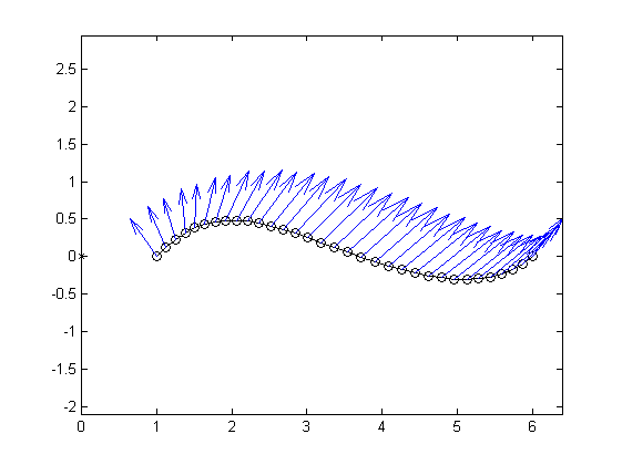
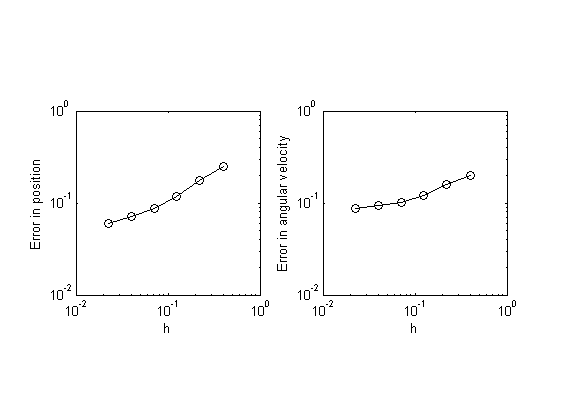
Figure 1. Left: Simulation of the method with $q_{0}=(1,0)$ $v_{0}=(1,1)$, $q_{N}=(6,0)$, $v_{N}=(1,1)$, $N=33$. Blue arrows show the (scaled) angular velocity. Right: Error (root-mean-square error) in position and angular velocity for different values of $h$.

The following table shows the root mean square error in positions and angular velocities

h Error in position Error in angular velocity

0.4 0.2471 0.1995

0.22 0.1746 0.1576

0.1250 0.1173 0.1204

0.0714 0.0866 0.1020

0.04 0.0705 0.0932

0.0225 0.0606 0.0875

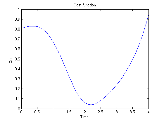
Figure 2. Cost function $\frac{1}{2}(u_{1}^{2}+u_{2}^{2})$

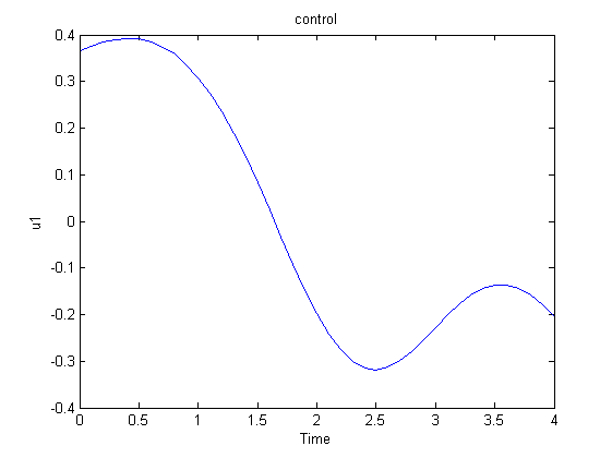
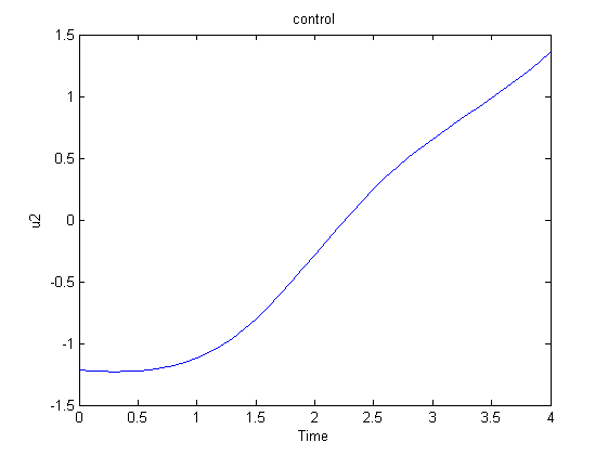
Figure 3. Controls $u_{1}$ and $u_{2}$

Observe that directly from construction the method is symplectic. We expect that this family of symplectic integrators could quantitative and qualitative benefit from structure preservation (see [12] and references therein).

Conclusions

In this paper, we have designed a new class of variational integrators for optimal control problems of underactuated mechanical systems, showing how developments in the theory of discrete mechanics and discrete calculus of variations with constraints can be used to construct numerical algorithms for optimal control problems with certain geometric desirable features,v(these features follow directly from the variational structure and were showed in [2], [5],[6], [15] and [16]. Also see Remark (4.2)).

We construct variational principles for higher-order systems with higher-order constraints (both in the continuous and discrete settings) and we use these developments to solve optimal control problems where the configuration space is a trivial principal bundle. From a discretization of Hamilton’s principle we derive the discrete version of the problem. We show two concrete applications of our ideas: the optimal control of an underactuated vehicle and a (homogeneous) ball rotating on a plate.

It is our intention to extend this construction to the case of non-trivial fiber bundles using a connection to split the reduced space [11].

Appendix: Retraction maps

In this appendix we will review the basics notions about retraction maps and the Cayley transformation (as an example of retraction map) which we use along this work.

A way to discretize a continuous problem is using a retraction map $\tau:{\mathfrak{g}}\to G$ which is an analytic local diffeomorphism. This application maps a neighborhood of $0\in{\mathfrak{g}}$ to a neighborhood of the identity $e\in G$. As a consequence, it is possible to deduce that $\tau(\xi)\tau(-\xi)=e$ for all $\xi\in\mathfrak{g}$.

The retraction map is used to express small discrete changes in the group configuration through unique Lie algebra elements (see [28]), namely $\xi_{k}=\tau^{-1}(g_{k}^{-1}g_{k+1})/h$, where $\xi_{k}\in\mathfrak{g}$. That is, if $\xi_{k}$ were regarded as an average velocity between $g_{k}$ and $g_{k+1}$, then $\tau$ is an approximation to the integral flow of the dynamics. The difference $g_{k}^{-1}\,g_{k+1}\in G$, which is an element of a nonlinear space, can now be represented by the vector $\xi_{k},$ in order to enable unconstrained optimization in the linear space $\mathfrak{g}$ for optimal control purposes.

It will be useful in the sequel, mainly in the derivation of the discrete equations of motion, to define the right trivialized tangent retraction map as a function $d\tau:\mathfrak{g}\times\mathfrak{g}\rightarrow\mathfrak{g}$ by

$$T\tau(\xi)\cdot\eta=Tr_{\tau(\xi)}d\tau_{\xi}(\eta),$$

where $\eta\in\mathfrak{g}$. Here we use the following notation, $d\tau_{\xi}:=d\tau(\xi):\mathfrak{g}\rightarrow\mathfrak{g}.$ The function $d\tau$ is linear in its second argument. From this definition the following identities hold (see [7] for further details)

Proposition: Given a map $\tau:\mathfrak{g}\rightarrow G$, its right trivialized tangent $d\tau_{\xi}:\mathfrak{g}\rightarrow\mathfrak{g}$ and its inverse $d\tau_{\xi}^{-1}:\mathfrak{g}\rightarrow\mathfrak{g}$, are such that for $g=\tau(\xi)\in G$ and $\eta\in\mathfrak{g}$, the following identities hold:

$$\partial_{\xi}\tau(\xi)\,\eta=\mbox{d}\tau_{\xi}\,\eta\,\tau(\xi)\,\,\hbox{ and }\,\,\partial_{\xi}\tau^{-1}(g)\,\eta=\mbox{d}\tau^{-1}_{\xi}(\eta\,\tau(-\xi)).$$

The most natural example of a retraction map is the exponential map at the identity $e$ of the group $G,$ $\mbox{exp}_{e}:\mathfrak{g}\rightarrow G$. We recall that, for a finite-dimensional Lie group, $\mbox{exp}_{e}$ is locally a diffeomorphism and gives rise to a natural chart [36]. Then, there exists a neighborhood $U$ of $e\in G$ such that $\mbox{exp}_{e}^{-1}:U\rightarrow\mbox{exp}_{e}^{-1}(U)$ is a local $\mathcal{C}^{\infty}-$diffeomorphism. A chart at $g\in G$ is given by $\Psi_{g}=\mbox{exp}_{e}^{-1}\circ\ell_{g^{-1}}.$

In general, it is not easy to work with the exponential map. In consequence it will be useful to use a different retraction map. More concretely, the Cayley map (see [7, 21] for further details) will provide us a proper framework in the examples shown along the paper.

The Cayley map

The Cayley map $\mbox{cay}:\mathfrak{g}\rightarrow G$ is defined by

$$\mbox{cay}(\xi)=(e-\frac{\xi}{2})^{-1}(e+\frac{\xi}{2})$$

and is valid for a class of quadratic groups (see [21] for example) that include the groups of interest in this paper (e.g. $SO(3)$, $SE(2)$ and $SE(3)$). Its right trivialized derivative and inverse are defined by

$$\mbox{d}\mbox{cay}_{x}\,y=(e-\frac{x}{2})^{-1}\,y\,(e+\frac{x}{2})^{-1},\quad\mbox{d}\mbox{cay}_{x}^{-1}\,y=(e-\frac{x}{2})\,y\,(e+\frac{x}{2}).$$

The Cayley map for $SE(2)$:

The coordinates on $SE(2)$ are $(\theta,x,y)$ with matrix representation for $g\in SE(2)$ given by

$$g=\left(\begin{array}[]{ccc}\mbox{cos}\,\theta&-\mbox{sin}\theta&x\\ \mbox{sin}\,\theta&\mbox{cos}\theta&y\\ 0&0&1\end{array}\right).$$

Using the isomorphic map $\hat{\cdot}:\mathds{R}^{3}\rightarrow\mathfrak{se}(3)$ given by

$$\hat{v}=\left(\begin{array}[]{ccc}0&-v_{1}&v_{2}\\ v_{1}&0&v_{3}\\ 0&0&0\end{array}\right),$$

where $v=(v_{1},v_{2},v_{2})^{T}\in\mathds{R}^{3}$, the set $\left\{\hat{e}_{1},\hat{e}_{2},\hat{e}_{3}\right\}$ can be used as a basis for $\mathfrak{se}(3)$, where $\left\{e_{1},e_{2},e_{3}\right\}$ is the standard basis of $\mathds{R}^{3}$. The map $\mbox{cay}:\mathfrak{se}(3)\rightarrow SE(2)$ is given by

$$\mbox{cay}(\hat{v})=\left(\begin{array}[]{c}\frac{1}{4+v_{1}^{2}}\left(\begin{array}[]{ccc}4-v_{1}^{2}&-4v_{1}&-2v_{1}v_{3}+4v_{2}\\ 4v_{1}&4-v_{1}^{2}&2v_{1}v_{2}+4v_{3}\end{array}\right)\\ \begin{array}[]{ccc}0&\,\,\,\,\,\,0&\,\,\,\,\,\,\,\,\,\,1\end{array}\end{array}\right),$$

while the map $\mbox{d}\tau_{\xi}^{-1}$ becomes the $3\times 3$ matrix

$$\mbox{d}\mbox{cay}_{\hat{v}}^{-1}=I_{3}-\frac{1}{2}\mbox{ad}_{v}+\frac{1}{4}\left(v_{1}v\,\,\,0_{3\times 2}\right),$$

where

$$\mbox{ad}_{v}=\left(\begin{array}[]{ccc}0&0&0\\ v_{3}&0&-v_{1}\\ -v_{2}&v_{1}&0\end{array}\right)$$

and $I_{3}$ denotes the $3\times 3$ identity matrix.

The Cayley map for $SO(3)$:

The group of rigid body rotations is represented by $3\times 3$ matrices with orthonormal column vectors corresponding to the axes of a right-handed frame attached to the body. On the other hand, the algebra $\mathfrak{so}(3)$ is the set of $3\times 3$ antisymmetric matrices. A $\mathfrak{so}(3)$ basis can be constructed as $\left\{\hat{e}_{1},\hat{e}_{2},\hat{e}_{3}\right\}$, $\hat{e}_{i}\in\mathfrak{so}(3)$, where $\left\{e_{1},e_{2},e_{3}\right\}$ is the standard basis for $\mathds{R}^{3}$. Elements $\xi\in\mathfrak{so}(3)$ can be identified with the vector $\omega\in\mathds{R}^{3}$ through $\xi=\omega^{\alpha}\,\hat{e}_{\alpha}$, or $\xi=\hat{\omega}$. Under such identification the Lie bracket coincides with the standard cross product, i.e., $\mbox{ad}_{\hat{\omega}}\,\hat{\rho}=\omega\times\rho$, for some $\rho\in\mathds{R}^{3}$. Using this identification we have

$$\mbox{cay}(\hat{\omega})=I_{3}+\frac{4}{4+\parallel\omega\parallel^{2}}\left(\hat{\omega}+\frac{\hat{\omega}^{2}}{2}\right),$$ (34)

where $I_{3}$ is the $3\times 3$ identity matrix. The linear maps $\mbox{d}\tau_{\xi}$ and $\mbox{d}\tau_{\xi}^{-1}$ are expressed as the $3\times 3$ matrices

$$\mbox{d}\mbox{cay}_{\omega}=\frac{2}{4+\parallel\omega\parallel^{2}}(2I_{3}+\hat{\omega}),\,\,\,\,\,\mbox{d}\mbox{cay}_{\omega}^{-1}=I_{3}-\frac{\hat{\omega}}{2}+\frac{\omega\,\omega^{T}}{4}.$$ (35)

References

• [1] J. Baillieul. The geometry of controlled mechanical systems. Mathematical control theory, Springer, New York, pp. 322–354, (1999).
• [2] R. Benito, M. de León and D. Martín de Diego. Higher-order discrete lagrangian mechanics Int. Journal of Geometric Methods in Modern Physics, 3, pp. 421–436, (2006).
• [3] A. Bloch. Nonholonomic Mechanics and Control. Interdisciplinary Applied Mathematics Series, Springer-Verlag, New-York, 24, (2003).
• [4] A.M. Bloch, I.I. Hussein, M. Leok and A.K. Sanyal. Geometric structure-preserving optimal control of a rigid body. Journal of Dynamical and Control Systems, 15(3), pp. 307–330, (2009)
• [5] N. Borda. Sistemas Mecánicos Discretos con Vínculos de orden 2, Master thesis, Instituto Balseiro, December 2011. avaiable at Borda
• [6] N. Borda, J. Fernandez, S. Grillo. Discrete second order constrained Lagrangian systems: First results. Journal Geometric Mechanics, Vol 5, n 4, 381-397 (2013).
• [7] N. Bou-Rabee and J.E. Marsden. Hamilton-pontryagin integrators on Lie groups. Foundations of Computational Mathematics, 9, pp. 197–219, (2009).
• [8] C. Burnett, D. Holm and D. Meier. Geometric integrators for higher-order mechanics on Lie groups, Proc. R. Soc. A. 469:20130249 (2013).
• [9] F. Bullo and A. Lewis. Geometric control of mechanical systems: Modeling, Analysis, and Design for Simple Mechanical Control Systems. Texts in Applied Mathematics, Springer Verlang, New York, (2005).
• [10] A. Castro and J. Koiller. On the dynamic Markov-Dubins problem: from path planning in robotics and biolocomotion to computational anatomy. Regul. Chaotic Dyn. 18 (2013), no. 1-2, 1 20.
• [11] H. Cendra, J. Marsden and T. Ratiu. Lagrangian reduction by stages. Memoirs of the American Mathematical Society, 152(722), pp. 1-108, (2001).
• [12] M. Chyba, E. Hairer and G. Vilmart. The role of symplectic integrators in optimal control. Opt. Control Appl. Method 30, 367 (2009).
• [13] L. Colombo, F. Jiménez and D. Martín de Diego. Discrete Second-Order Euler-Poincaré Equations. An application to optimal control. International Journal of Geometric Methods in Modern Physics, 9(4), 20 pp., (2012).
• [14] L. Colombo, D. Martín de Diego and M. Zuccalli. Optimal Control of Underactuated Mechanical Systems: a geometric approach. Journal of Mathematical Physics, 51, 24 pp., (2010).
• [15] L. Colombo, D. Martín de Diego and M. Zuccalli. On variational integrators for optimal control of mechanical systems. RACSAM Rev. R. Acad. Cienc. Ser A. Mat, (2011).
• [16] L. Colombo L, D. Martín de Diego and M. Zuccalli. Higher-order variational problems with constraints. Journal of Mathematical Physics. Vol 54, 093507 (2013).
• [17] J. Cortés, M. de León, J.C. Marrero and E. Martínez. Nonholonomic Lagrangian systems on Lie algebroids. Discrete and Continuous Dynamical Systems - Series A, 24 (2), pp. 213–271, (2009).
• [18] F. Gay-Balmaz, D. Holm and T. Ratiu. Higher order Lagrange-Poincaré, and Hamilton-Poincaré reductions. Bulletin of the Brazialian Mathematical Society, 42, pp. 579-606, (2011).
• [19] F. Gay-Balmaz, D. D. Holm and T. S. Ratiu. Geometric dynamics of optimization. Comm. Math. Sci., 11(1), pp. 163–231, (2012).
• [20] F. Gay-Balmaz, D. D. Holm, D. M. Meier, T. S. Ratiu and F.-X. Vialard. Invariant higher-order variational problems. Communications in Mathematical Physics, 309(2), pp. 413–458, (2012).
• [21] E. Hairer, C. Lubich and G. Wanner. Geometric Numerical Integration, Structure-Preserving Algorithms for Ordinary Differential Equations. Springer Series in Computational Mathematics, Springer-Verlag, Berlin, 31, (2002).
• [22] D. D. Holm. Geometric mechanics. Part I and II. Imperial College Press, London; distributed by World Scientific Publishing Co. Pte. Ltd., Hackensack, NJ, (2008).
• [23] F. Jiménez, M. de León and D. Martín de Diego. Hamiltonian dynamics and constrained variational calculus: Continuous and discrete settings J. Phys A, Vol 45, 205204 (2012).
• [24] F. Jiménez, M. Kobilarov and D. Martín de Diego. Discrete variational optimal control. Journal of Nonlinear Science, 23(3), pp. 393–426, (2013).
• [25] F. Jiménez and D. Martín de Diego. A geometric approach to Discrete mechanics for optimal control theory. Proceedings of the IEEE Conference on Decision and Control, Atlanta, Georgia, USA, pp. 5426–5431, (2010).
• [26] M. Kobilarov and J.E. Marsden. Discrete Geometric Optimal Control on Lie Groups. IEEE Transactions on Robotics, 27(4), pp. 641–655, (2011).
• [27] M. Kobilarov. Discrete Geometric Motion Control of Autonomous Vehicles. Thesis, University of Southern California, Computer Science, (2008).
• [28] M. Kobilarov and J. Marsden. Discrete Geometric Optimal Control on Lie Groups. IEEE Transactions on Robotics, 27(4), pp. 641–655, (2011).
• [29] W-S. Koon. Reduction, Reconstruction and Optimal Control for Nonholonomic Mechanical Systems with Symmetry. PhD thesis, University of California, Berkeley, (1997).
• [30] T. Lee, M. Leok and N. H. McClamroch. Optimal Attitude Control of a Rigid Body using Geometrically Exact Computations on $SO(3)$. Journal of Dynamical and Control Systems, 14(4), pp. 465–487 (2008).
• [31] M. Leok. Foundations of Computational Geometric Mechanics, Control and Dynamical Systems. Thesis, California Institute of Technology, 2004. Available in Leok.
• [32] M. de León and P. R. Rodrigues. Generalized Classical Mechanics and Field Theory. North-Holland Mathematical Studies, North-Holland, Amsterdam, 12, (1985).
• [33] A. Lewis and R. Murray. Variational principles for constrained systems: Theory and experiment. Int. J. Nonlinear Mechanics, 30(6), pp. 793–815, (1998).
• [34] J.C. Marrero, D. Martín de Diego D and E. Martínez. Discrete Lagrangian and Hamiltonian Mechanics on Lie groupoids. Nonlinearity, 19(6), pp. 1313–1348, (2006).
• [35] J. C. Marrero, D. Martín de Diego and A. Stern. Symplectic groupoids and discrete constrained Lagrangian systems. arXiv: 1103.6250, (2011).
• [36] J. Marsden, S. Pekarsky and S. Shkoller. Discrete Euler-Poincaré and Lie-Poisson equations. Nonlinearity, 12, pp. 1647–1662, (1999).
• [37] J.E. Marsden and J.M. Wendlandt. Mechanical Integrators Derived from a Discrete Variational Principle Physica D, 106, pp. 223–246, (1997).
• [38] J. Marsden and M. West. Discrete Mechanics and variational integrators. Acta Numerica, 10, pp. 357–514, (2001).
• [39] D. Meier. Invariant higher-order variational problems: Reduction, geometry and applications. Ph.D thesis, Imperial College London (2013).
• [40] S. Ober-Blöbaum, O. Junge and J. Marsden. Discrete Mechanics and Optimal Control: an Analysis. ESAIM: COCV, 17(2), pp. 322–352, (2011).