New Mixing Structures of Chiral Generations in a Model with Noncompact Horizontal Symmetry

Abstract

New mixing structures between chiral generations of elementary particles at low energy are shown in a vectorlike model with a horizontal symmetry $SU(1,1)$. In this framework the chiral model including odd number chiral generations is realized via the spontaneous symmetry breaking of the horizontal symmetry. It is shown that the Yukawa coupling matrices of chiral generations have naturally hierarchical patterns, and in some cases the overall factors of their Yukawa coupling matrices, e.g. the Yukawa coupling constants of the bottom quark and tau lepton are naturally suppressed.

1 Introduction

One of the most remarkable phenomena in Nature at low energies is the existence of three chiral generations of quarks and leptons and their hierarchical mass structures. There have been many attempts to understand the origin of generations and/or the hierarchical structures by using various models; e.g. models with horizontal symmetries $G_{H}$ [1, 2, 3, 4], which govern the generational structures of quarks and leptons; grand unified models on the orbifold $S^{1}/Z_{2}$ [5, 6]; nonlinear $\sigma$ models on the coset space $E_{7(+7){\rm global}}/SU(5)\times U(1)^{3}$ [7, 8]; and magnetized orbifolding models [9, 10, 11].

We focus on approaches based on horizontal symmetries. These symmetries can be classified into three categories. First, models with non-abelian group symmetries [12, 13] give an explanation for the three generations of quarks and leptons if the group involves a triplet representation. Second, models with an abelian group $U(1)$ [2, 14] naturally gives an account for the hierarchical mass structures of the three chiral generations of quarks and leptons by using the Froggatt-Nielsen mechanism [2]. Third, a model with a noncompact nonabelian group symmetry $SU(1,1)$ [15] allows us the opportunity that chiral generations of elementary particles and their hierarchical mass structures are understood by using the spontaneous symmetry breaking, one of the essential concepts of modern particle physics, of the horizontal symmetry, where the noncompact group $SU(1,1)$ is a special pseudo-unitary group [16, 17]. (Another example of a special pseudo-unitary group is the Lorentz group $SO(3,1)$.)

The author has previously discussed an $\mathcal{N}=1$ supersymmetric vectorlike model with a noncompact group $SU(1,1)$ horizontal symmetry [18, 19]. This model has some important features: chiral gauge theories derived from vectorlike gauge theories [15]; the hierarchical structure of Yukawa coupling constants of chiral matter at low energy [18]; and the spontaneous breakdown of P, C and T symmetries [19]. Once we apply this model to the standard model (SM), these features can realize almost the constrained minimal supersymmetric standard model (MSSM) [20, 21] at low energy [19]. See Ref. [22] for a review.

The main purpose of this paper is to show new types of structures to realize chiral generations of elementary particles at low energy in a model with the horizontal symmetry $SU(1,1)$. In some cases the pattern of the Yukawa coupling constants of the chiral generations derived from the new structures is much different from that discussed before. The difference between the Yukawa coupling constants of top quarks, bottom quarks and tau leptons is also discussed. In §2 we give an overview of the noncompact horizontal symmetry and define the terms of the model. In §3 we discuss how to realize chiral generations in the context of the known structure and the new structure. In §4 we analyze typical Yukawa coupling structures by using the mixing patterns of chiral generations in §3. Section 5 is devoted to summary and discussion.

2 Overview of the Model

We give an overview of the noncompact horizontal symmetry $SU(1,1)$ and define the terms of the model. Let us begin by defining the three generators $\tau_{a}$ $(a=1,2,3)$ of $SU(1,1)$ satisfying the commutation relations

$$[\tau_{1},\tau_{2}]=-i\tau_{3},\ \ \ [\tau_{2},\tau_{3}]=+i\tau_{1},\ \ \ [\tau_{3},\tau_{1}]=+i\tau_{2}.$$ (1)

The components of any representation of $SU(1,1)$ are labeled by the Casimir operator $\mathbf{\tau}^{2}$ of $SU(1,1)$ and the weight of the third component $\tau_{3}$ of $SU(1,1)$, where the Casimir operator of $SU(1,1)$ is defined by $\mathbf{\tau}^{2}:=\tau_{1}^{2}+\tau_{2}^{2}-\tau_{3}^{2}$.

We use two types of representations of $SU(1,1)$; one type is unitary infinite-dimensional representations, which are constructed using all Hermitian generators $\tau_{a}$; the other type is nonunitary finite-dimensional representations, which are constructed using two anti-Hermitian generators $\tau_{1}$ and $\tau_{2}$ and one Hermitian generator $\tau_{3}$. Two types of infinite-dimensional representations are used; one representation has only positive weights of the third component generator $\tau_{3}$, where the lowest state is vanished by the ladder operator $\tau_{-}:=\tau_{1}-i\tau_{2}$; the other has only negative weights of the third component generator $\tau_{3}$, where the highest state is vanished by the ladder operator $\tau_{+}:=\tau_{1}+i\tau_{2}$. A field in the representation with only a positive weight is referred to as a positive field denoted by, e.g., $\hat{F}=\{\hat{f}_{\alpha},\hat{f}_{\alpha+1},\cdots\}$, where the subscripts of the components $\hat{f}_{\alpha+i}$ $(i=0,1,2,\cdots)$ of $\hat{F}$ stand for the weight of $\tau_{3}$ of $SU(1,1)$. A field in the representation with only a negative weight is referred as a negative field denoted by, for example, $\hat{F}^{c}=\{\hat{f}^{c}_{-\alpha},\hat{f}^{c}_{-\alpha-1},\cdots\}$. The finite-dimensional representations are characterized by the highest weight $S$ referred to as the $SU(1,1)$ spin $S$ and the weight of eigenvalue of the third component generator $\tau_{3}$, where the highest state is vanished by the operator $\tau_{+}$, and the lowest state is vanished by the operator $\tau_{-}$. A field in a finite-dimensional representation is referred to as a finite field denoted by, e.g., $\hat{\Psi}=\{\hat{\psi}_{-S},\hat{\psi}_{-S+1},\cdots,\hat{\psi}_{S-1},\hat{\psi}_{S}\}$, where the subscripts of the components $\hat{\psi}_{n}$ $(n=-S,-S+1,\cdots,S)$ of the finite field $\hat{\Psi}$ stand for the weight of $\tau_{3}$, and $S$ is a non-negative integer or a half-integer. In the following, we refer to the positive and negative fields introduced in a vectorlike manner as matter fields, such as quarks, leptons and higgses. The finite fields are referred to as structure fields because these determine the generational structures of the model and do not correspond to the SM or supersymmetric SM fields.

Before we finish this section, we introduce two cubic invariants under $SU(1,1)$ transformations [18]; one is built from two infinite dimensional unitary representations with one positive and one negative weight and finite-dimensional representations; the other consists of three infinite-dimensional unitary representations with two positive weights and one negative weight, or one positive weight and two negative weights. The former is the following cubic coupling term

$$\hat{F}\hat{G}^{c}\hat{\Psi}=\sum_{i,j=0}^{\infty}D^{\beta,\alpha,S}_{j,i}\ \hat{f}_{\alpha+i}\hat{g}^{c}_{-\beta-j}\hat{\psi}_{-i+j-q},$$ (2)

where $\alpha(-\beta)$ is the lowest(highest) weight of the matter field $\hat{F}(\hat{G}^{c})$, and $q$ is defined as $q:=\alpha-\beta$ and is an integer or half-integer, which is allowed when the $SU(1,1)$ spin $S$ of the structure field $\hat{\Psi}$ satisfies $S\geq|q|$. For $S\geq|-i+j-q|$, the Clebsch-Gordan coefficient (CGC) is

$$D^{\beta,\alpha,S}_{j,i} =(-1)^{i}\sqrt{\frac{i!j!(i-j+S+q)!(-i+j+S-q)!}{\Gamma(2\alpha+i)\Gamma(2\beta+j)}}$$

$$\times\sum_{r=0}^{S+q}\frac{\Gamma(2\beta+j+r)}{(S+q-r)!(i-j+S+q-r)!r!(-i+j-2q+r)!(j-S-q+r)!}~{};$$ (3)

otherwise, $D^{\beta,\alpha,S}_{j,i}=0$. The CGC $D_{j,i}^{\beta,\alpha,S}$ satisfies the symmetric relation $D_{j,i}^{\beta,\alpha,S}=(-1)^{i-j}D_{i,j}^{\alpha,\beta,S}$. The CGC $D_{j,i}^{\beta,\alpha,S}$ of the matter and structure fields $\hat{F}\hat{F}^{c}\hat{\Psi}$ behaves as $i^{S}$ in the limit $i,j\to\infty$ with $|i-j|$ fixed:

$$D_{j,i}^{\beta,\alpha,S}\simeq(-1)^{i}i^{S}\frac{(2S)!}{(S+q)!(S-q)!\sqrt{(i-j+S-q)!(-i+j+S+q)!}}.$$ (4)

As we find in §3, this asymptotic behavior is essential to realize chiral theories from vectorlike theories. The latter is

$$\hat{F}\hat{G}\hat{H}=\sum_{i,j=0}^{\infty}C_{i,j}^{\alpha,\beta,\Delta}\hat{f}_{\alpha+i}\hat{g}_{\beta+j}\hat{h}_{-\gamma-i-j+\Delta},$$ (5)

where $\Delta$ is a semi-positive integer $(\Delta\geq 0)$. For $i+j<\Delta$, the CGC is zero and, for $i+j\geq\Delta$,

$$C_{i,j}^{\alpha,\beta,\Delta}= (-1)^{i+j}\sqrt{\frac{i!j!}{(i+j-\Delta)!}\frac{\Gamma(2\alpha+i)\Gamma(2\beta+j)}{\Gamma(2\gamma+i+j+\Delta)}}$$

$$\times\sum_{r=0}^{\Delta}(-1)^{r}\frac{(i+j-\Delta)!\Gamma(2\alpha)\Gamma(2\beta)}{(i-r)!(j+r-\Delta)!r!(\Delta-r)!\Gamma(2\alpha+r)\Gamma(2\beta+\Delta-r)},$$ (6)

where the $C_{i,j}^{\alpha,\beta,\Delta}$ satisfies the symmetric relation $C_{i,j}^{\alpha,\beta,\Delta}=(-1)^{\Delta}C_{j,i}^{\beta,\alpha,\Delta}$.

3 Spontaneous Generation of Generations

We now discuss how to extract chiral matter content from vectorlike matter content. This mechanism is referred to as the spontaneous generation of generations [15]. The mechanism can produce finite numbers of chiral generations of the SM fields at low energies, such as quarks, from matter fields, where matter fields belong to the infinite-dimensional representation of $SU(1,1)$ in a vectorlike manner. The appearance of chiral generations of matter is dominantly dependent on the $SU(1,1)$ spins of the structure fields $\hat{\Psi}$s with non-vanishing vacuum expectation values (VEVs) and subdominantly depends on certain combinations of the VEVs of the structure fields $\hat{\Psi}$s and coupling constants, because of normalizable condition of chiral particles.

We first investigate the superpotential that includes two structure fields with integer spins discussed in Ref. [23, 18]. After that, the superpotential that includes a structure field with a half-integer spin is discussed.

3.1 Two Structure Fields with an Integer Spin

We consider the superpotential that contains the matter fields $\hat{F}$ and $\hat{F}^{c}$ and the structure fields $\hat{\Psi}$ and $\hat{\Psi}^{\prime}$

$$W=x\hat{F}\hat{F}^{c}\hat{\Psi}+x^{\prime}\hat{F}\hat{F}^{c}\hat{\Psi}^{\prime},$$ (7)

where $x$ and $x^{\prime}$ are real coupling constants. We assume non-vanishing VEVs for the $0$th and $-g$th components of the structure fields $\hat{\Psi}$ and $\hat{\Psi}^{\prime}$ with the $SU(1,1)$ spins $S$ and $S^{\prime}$, respectively, and assume that the scale of these VEVs is a high energy scale such as the GUT scale or Planck scale and the typical energy scale of massless matter is a low scale such as the electroweak scale. The non-vanishing VEVs $\langle\psi_{0}\rangle$ and $\langle\psi_{-g}^{\prime}\rangle$ can generate $g$ massless modes $\{\hat{f}_{0},\hat{f}_{1},\hat{f}_{2},\cdots,\hat{f}_{g-1}\}$ $(S^{\prime}\geq g)$ from the positive field $\hat{F}$ with the form

$$\hat{f}_{\alpha+i}=\sum_{n=0}^{g-1}\hat{f}_{n}U_{n,i}^{f}+[\mbox{massive modes}],$$ (8)

where $\hat{f}_{\alpha+i}$ $(i=0,1,2,\cdots)$ are the components of the positive field $\hat{F}$ whose lowest weight is $\alpha$, $\hat{f}^{c}_{-\alpha-i}$ are only massive modes, and $U_{n,i}^{f}$ is referred to as the mixing coefficient of the matter field $\hat{F}$. The coefficient represents the relation between the eigenstates of the third component generator of $SU(1,1)$ and mass eigenstates of massless modes.

Let us calculate the mass term of the superpotential in Eq. (7) at the vacuum to obtain the massless and chiral matter fields. Substituting the modes in Eq. (8) for the superpotential in Eq. (7), we obtain

$$\left.W\right|_{\Psi=\langle\Psi\rangle} =x\hat{F}\hat{F}^{c}\langle\hat{\Psi}\rangle+x^{\prime}\hat{F}\hat{F}^{c}\langle\hat{\Psi}^{\prime}\rangle$$

$$=\sum_{i=0}^{\infty}\left(xD_{i,i}^{\alpha,\alpha,S}\langle\psi_{0}\rangle\hat{f}_{\alpha+i}\hat{f}^{c}_{-\alpha-i}+x^{\prime}D_{i,i+g}^{\alpha,\alpha,S^{\prime}}\langle\psi_{-g}^{\prime}\rangle\hat{f}_{\alpha+i+g}\hat{f}^{c}_{-\alpha-i}\right)$$

$$=\sum_{i=0}^{\infty}\hat{f}_{n}\left(xD_{i,i}^{\alpha,\alpha,S}\langle\psi_{0}\rangle U_{n,i}^{f}+x^{\prime}D_{i,i+g}^{\alpha,\alpha,S^{\prime}}\langle\psi_{-g}^{\prime}\rangle U_{n,i+g}^{f}\right)\hat{f}^{c}_{-\alpha-i}+[\mbox{massive modes}],$$ (9)

where $D_{i,i}^{\alpha,\alpha,S}$ and $D_{i,i+g}^{\alpha,\alpha,S^{\prime}}$ are CGCs of the positive-negative-finite field coupling defined in Eq. (3).

The massless modes $\hat{f}_{n}$ are extracted from the component $\hat{f}_{\alpha+i}$ of the matter field $\hat{F}$. The orthogonality of the massless modes $\hat{f}_{n}$ to the massive modes $\hat{f}_{-\alpha-i}^{c}$ requires the coefficients $U_{n,i}^{f}$ to satisfy the recursion equation

$$x\langle\psi_{0}\rangle D_{i,i}^{\alpha,\alpha,S}U_{n,i}^{f}+x^{\prime}\langle\psi_{-g}^{\prime}\rangle D_{i,i+g}^{\alpha,\alpha,S^{\prime}}U_{n,i+g}^{f}=0.$$ (10)

This equation gives the mixing coefficients

$$U^{f}_{n,i}=U^{f}_{n}\sum_{s=0}^{\infty}\delta_{i,n+gs}(-\epsilon)^{s}b^{f}_{n,s},\ \ \ \ \epsilon=\frac{x\langle\psi_{0}\rangle}{x^{\prime}\langle\psi_{-g}^{\prime}\rangle},\ \ \ b^{f}_{n,s}=\prod_{r=0}^{s-1}\frac{D^{\alpha,\alpha,S}_{gr+n,gr+n}}{D^{\alpha,\alpha,S^{\prime}}_{gr+n,g(r+1)+n}},$$ (11)

where $n=0,1,2,\cdots g-1$, and the parameter $\epsilon$ depends on the couplings and the VEVs. The $b_{n,s}^{f}$ is determined by the weights of the $SU(1,1)$ $\alpha$ and $S$, where $b_{n,0}^{f}:=1$.

To understand the meaning of the mixing coefficient in Eq. (11), we first examine two extreme cases of VEVs; $\langle\psi_{0}\rangle=0$ and $\langle\psi_{-g}^{\prime}\rangle\not=0$; and $\langle\psi_{0}\rangle\not=0$ and $\langle\psi_{-g}^{\prime}\rangle=0$. In the case of the VEVs $\langle\psi_{0}\rangle=0$ and $\langle\psi_{-g}^{\prime}\rangle\not=0$, the recursion equation in Eq. (10) constrains the mixing coefficients $U_{n,i+g}^{f}=0$ $(i=0,1,2,\cdots)$ and does not determine $U_{n,k}^{f}$ $(k=1,2,\cdots,g-1)$, and we take a normalization condition $U_{n,i}^{f}=\delta_{n,i}$. This means that the component $\hat{f}_{\alpha+n}$ $(n=0,1,\cdots,g-1)$ can be identified as its corresponding massless mode $\hat{f}_{n}$. For example, for $g=3$, from Fig. 1, since the components $\hat{f}_{\alpha}$, $\hat{f}_{\alpha+1}$ and $\hat{f}_{\alpha+2}$ do not have any mass term, they are massless. The other components $\hat{f}_{\alpha+3+i}$ and $\hat{f}_{-\alpha-i}^{c}$ $(i=0,1,2,\cdots)$ have a corresponding mass $x^{\prime}D_{i,i+3}^{\alpha,\alpha,S^{\prime}}\langle\psi_{-3}^{\prime}\rangle$, they are massive. Three massless modes appear, and they can be identified as $\hat{f}_{0}=\hat{f}_{\alpha}$, $\hat{f}_{1}=\hat{f}_{\alpha+1}$ and $\hat{f}_{2}=\hat{f}_{\alpha+2}$. Next, in the case of the VEVs $\langle\psi_{0}\rangle\not=0$ and $\langle\psi_{-g}^{\prime}\rangle=0$, the recursion equation in Eq. (10) determines the mixing coefficients satisfying $U_{n,i}^{f}=0$ $(i=0,1,2,\cdots)$ and from Fig. 2, since all the components $\hat{f}_{\alpha+i}$ and $\hat{f}_{-\alpha-i}^{c}$ have a mass term, no massless modes emerge.

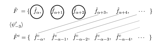
Figure 1: An example for the three massless generation case assuming the VEVs $\langle\psi_{0}\rangle=0$ and $\langle\psi_{-g}^{\prime}\rangle\not=0$ and $g=3$ in Eq. (9): the components $\hat{f}_{\alpha}$, $\hat{f}_{\alpha+1}$ and $\hat{f}_{\alpha}$ of the matter field $\hat{F}$ are massless, and the other components of $\hat{F}$ and all the components of $\hat{F}^{c}$ are massive, where the massless modes are surround by a circle, and the components $\hat{f}_{\alpha+3+i}$ and $\hat{f}_{-\alpha-i}^{c}$ $(i=0,1,2,\cdots)$ of the matter fields $\hat{F}$ and $\hat{F}^{c}$ connected by a solid line have a mass term that comes from the VEV $\langle\psi_{-3}^{\prime}\rangle$.

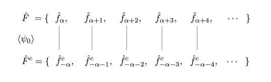
Figure 2: An example for the no massless generation case assuming the VEVs $\langle\psi_{0}\rangle\not=0$ and $\langle\psi_{-g}^{\prime}\rangle=0$ in Eq. (9): all the components of the matter fields $\hat{F}$ and $\hat{F}^{c}$ are massive, where all the components $\hat{f}_{\alpha+i}$ and $\hat{f}_{-\alpha-i}^{c}$ $(i=0,1,2,\cdots)$ of the matter fields $\hat{F}$ and $\hat{F}^{c}$ connected by a solid line have a mass term that comes from the VEV $\langle\psi_{0}\rangle$.

Let us move on to the case of the VEVs $\langle\psi_{0}\rangle\not=0$ and $\langle\psi_{-g}^{\prime}\rangle\not=0$ in Eqs. (10) and (11). From the above consideration for the cases of $\langle\psi_{0}\rangle=0$ or $\langle\psi_{-g}^{\prime}\rangle=0$, in the case of the VEVs $\langle\psi_{0}\rangle\not=0$ and $\langle\psi_{-g}^{\prime}\rangle\not=0$, we expect that the massless mode $\hat{f}_{n}$ $(n=0,1,\cdots,g-1)$ that is realized by certain linear combinations of the components $\hat{f}_{\alpha+gk+n}$ $(k=1,2,\cdots)$ appears as in Fig. 3 or no massless mode appears as in Fig. 4. In fact the realization of the massless modes $\hat{f}_{n}$ $(n=0,1,\cdots,g-1)$ requires a normalizable condition $\sum_{i=0}^{\infty}|U_{n,i}^{f}|^{2}<\infty$; if this condition is not satisfied, the massless modes $\hat{f}_{n}$ are illusions without any physical reality. Since the mixing coefficients in Eq. (11) are a geometric series, the requirement of the normalizable condition corresponds to the condition

$$\lim_{i\rightarrow\infty}\left|\frac{U_{n,i+g}^{f}}{U_{n,i}^{f}}\right|<1.$$ (12)

By using the asymptotic behavior of the CGC $D_{j,i}^{\beta,\alpha,S}$ in Eq. (4), we find

$$\lim_{i\rightarrow\infty}\left[\left|\frac{U_{n,i+g}^{f}}{U_{n,i}^{f}}\right|-\left|\frac{\epsilon}{\epsilon_{cr}}\right|i^{S-S^{\prime}}\right]=0,$$ (13)

where $\epsilon_{cr}$ is a constant that is dependent on the $SU(1,1)$ spins and the number of generations and is independent of the component $i$. Thus, the requirement of the normalizable condition is dominantly determined by the relation between the $SU(1,1)$ spins $S$ and $S^{\prime}$ and subdominantly depends on the relation between $\epsilon$ and $\epsilon_{cr}$.

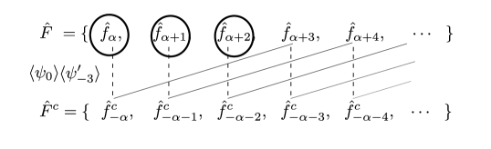
Figure 3: An example for the three massless generation case $g=3$ in Eq. (9): each massless mode $\hat{f}_{n}$ $(n=0,1,2)$ is realized by certain linear combinations of the components $\hat{f}_{\alpha+3k+n}$ $(k=1,2,\cdots)$, and the constructional element of each massless mode is determined by its mixing coefficients $U_{n,n+3k}^{f}$ given in Eq. (11), where the components of the matter fields $\hat{F}$ and $\hat{F}^{c}$ connected by solid and dashed lines have mass terms that come from the VEVs $\langle\psi_{-3}^{\prime}\rangle$ and $\langle\psi_{0}\rangle$, respectively, and the mass term of the solid line that comes from the VEV $\langle\psi_{-3}^{\prime}\rangle$ dominantly contributes to whether massless modes appear or not.

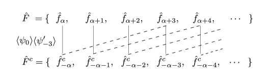
Figure 4: An example for the no massless generation case $g=3$ in Eq. (9), where the components of the matter fields $\hat{F}$ and $\hat{F}^{c}$ connected by solid and dashed lines have mass terms that comes from the VEVs $\langle\psi_{0}\rangle$ and $\langle\psi_{-3}^{\prime}\rangle$, respectively, and the mass term of the solid line that comes from the VEV $\langle\psi_{0}\rangle$ dominantly contributes to whether massless modes appear or not.

Whether massless generations appear or not can be classified into three types by using the $SU(1,1)$ spins $S$ and $S^{\prime}$ of the structure fields $\hat{\Psi}$ and $\hat{\Psi}^{\prime}$, respectively: $S>S^{\prime}$, $S<S^{\prime}$ and $S=S$. First, for $S>S^{\prime}$, since $\lim_{i\to\infty}|U_{n,i+g}^{f}/U_{n,i}^{f}|=0$, the normalizable condition in Eq. (12) is always satisfied. Thus, the massless modes $\hat{f}_{n}$ appear as in Fig. 3 for any value of the parameter $\epsilon$. Next, for $S<S^{\prime}$, since $\lim_{i\to\infty}|U_{n,i+g}^{f}/U_{n,i}^{f}|=\infty$, the normalizable condition in Eq. (12) is not satisfied. Thus, no massless mode appear as in Fig. 4 for any value of the parameter $\epsilon$. Finally, for $S=S^{\prime}$, whether the normalizable condition is satisfied and which situation occurs as in Fig. 3 or Fig. 4 depend on the parameter $\epsilon$ because $\lim_{i\to\infty}|U_{n,i+g}^{f}/U_{n,i}^{f}|=|\epsilon/\epsilon_{cr}|$. The condition $S=S^{\prime}$ is referred to as a marginal assignment. The critical value $\epsilon_{cr}$ can be calculated by using the mixing coefficient in Eq. (11) and the asymptotic form of the CGC $D_{j,i}^{\beta,\alpha,S}$ in Eq. (4); the parameter $\epsilon$ must satisfy the constraint

$$|\epsilon|<\epsilon_{cr}=\sqrt{\frac{S!S!}{(S+g)!(S-g)!}}$$ (14)

to produce the massless modes $\hat{f}_{n}$.

The chiral nature of supersymmetry plays an important role in this model. If the model is not based on supersymmetry and matter fields $F$ and $F^{c}$ are spin-$1/2$ fermions and a structure field $\Psi^{\prime}$ is a spin-$0$ boson, then a Yukawa coupling term $FF^{c}\Psi^{\prime}$ is allowed by gauge symmetry and the conjugate term $FF^{c}\Psi^{\prime{\dagger}}$ is also permitted because the structure field $\Psi^{\prime}$ belongs to the real representation of $SU(1,1)$. The latter term destroys the chiral structures and all massless modes disappear at low energy. Supersymmetry naturally forbids the latter coupling by its chiral nature.

3.2 One Structure Field with an Integer Spin and One with a Half-Integer Spin

Let us start to discuss the structures of the massless modes in a model with structure fields with an integer spin and a half-integer spin. We introduce an additional set of the matter fields $\hat{F}^{\prime}$ and $\hat{F}^{\prime}{}^{c}$ with the lowest weight $\alpha^{\prime}$ and the highest weight $-\alpha^{\prime}$, respectively. We choose the value

$$q:=\alpha^{\prime}-\alpha$$ (15)

to be a positive half-integer. We suppose that massless generations are realized as a linear combination of the components of the matter fields $\hat{F}$ and $\hat{F}^{\prime}$

$$\hat{f}_{\alpha+i}=\sum_{n=0}\hat{f}_{n}U^{f}_{n,i}+[{\rm massive\ modes}],\ \ \ \hat{f}_{\alpha^{\prime}+i}^{\prime}=\sum_{n=0}\hat{f}_{n}U_{n,i}^{f\prime}+[{\rm massive\ modes}],$$ (16)

and the conjugate fields $\hat{f}_{-\alpha-i}^{c}$ and $\hat{f}_{-\alpha^{\prime}-i}^{\prime c}$ do not include these massless modes, where $n$ is a label of these massless modes. We also introduce two structure fields $\hat{\Phi}$ and $\hat{\Psi}$ with an $SU(1,1)$ integer spin $S$ and an $SU(1,1)$ half-integer spin $S^{\prime}$, respectively. They couple to the matter fields in the following form

$$W =x\hat{F}\hat{F}^{c}\hat{\Phi}+x^{\prime}\hat{F}^{\prime}\hat{F}^{\prime}{}^{c}\hat{\Phi}+z\hat{F}^{\prime}\hat{F}^{c}\hat{\Psi}+z^{\prime}\hat{F}\hat{F}^{\prime}{}^{c}\hat{\Psi},$$ (17)

where $x,x^{\prime},z,z^{\prime}$ are coupling constants and $q$ must be less than or equal to $S^{\prime}$ $(q\leq S^{\prime})$ to realize the superpotential.

We discuss how many generations of matter fields $\hat{f}_{n}$ are produced from a double matter sector through the superpotential in Eq. (17). We assume that the $0$th and $-p$th $(p>0)$ components of the structure fields $\hat{\Phi}$ and $\hat{\Psi}$ acquire non-vanishing VEVs:

$$\langle\hat{\Phi}\rangle=\langle\phi_{0}\rangle,\hskip 10.00002pt\langle\hat{\Psi}\rangle=\langle\psi_{-p}\rangle,$$ (18)

where $p$ must be less than or equal to $S^{\prime}$ $(p\leq S^{\prime})$.

We calculate the mass term of the superpotential in Eq. (17) to confirm how much massless matter emerges in the low energy physics. By substituting the expressions in Eq. (18) into the mass term in Eq. (17) at the vacuum, we have

$$\left.W\right|_{\Psi=\langle\Psi\rangle} =x\hat{F}\hat{F}^{c}\langle\hat{\Phi}\rangle+x^{\prime}\hat{F}^{\prime}\hat{F}^{\prime}{}^{c}\langle\hat{\Phi}\rangle+z\hat{F}^{\prime}\hat{F}^{c}\langle\hat{\Psi}\rangle+z^{\prime}\hat{F}\hat{F}^{\prime}{}^{c}\langle\hat{\Psi}\rangle$$

$$=\sum_{i=0}^{\infty}\bigg{[}xD_{i,i}^{\alpha,\alpha,S}\langle\phi_{0}\rangle\hat{f}_{\alpha+i}\hat{f}_{-\alpha-i}^{c}+x^{\prime}D_{i,i}^{\alpha^{\prime},\alpha^{\prime},S}\langle\phi_{0}\rangle\hat{f}_{\alpha^{\prime}+i}^{\prime}\hat{f}_{-\alpha^{\prime}-i}^{\prime c}$$

$$\hskip 20.00003pt+zD_{i,i+p-q}^{\alpha,\alpha^{\prime},S^{\prime}}\langle\psi_{-p}\rangle\hat{f}_{\alpha^{\prime}+i+p-q}^{\prime}\hat{f}_{-\alpha-i}^{c}+z^{\prime}D_{i,i+p+q}^{\alpha^{\prime},\alpha,S^{\prime}}\langle\psi_{-p}\rangle\hat{f}_{\alpha+i+p+q}\hat{f}_{-\alpha^{\prime}-i}^{\prime c}\bigg{]}$$

$$=\sum_{n=0}\sum_{i=0}^{\infty}\bigg{[}\hat{f}_{n}\left(xD_{i,i}^{\alpha,\alpha,S}\langle\phi_{0}\rangle U^{f}_{n,i}+zD_{i,i+p-q}^{\alpha,\alpha^{\prime},S^{\prime}}\langle\psi_{-p}\rangle U_{n,i+p-q}^{f\prime}\right)\hat{f}_{-\alpha-i}^{c}$$

$$+\hat{f}_{n}\left(x^{\prime}D_{i,i}^{\alpha^{\prime},\alpha^{\prime},S}\langle\phi_{0}\rangle U_{n,i}^{f\prime}+z^{\prime}D_{i,i+p+q}^{\alpha^{\prime},\alpha,S^{\prime}}\langle\psi_{-p}\rangle U^{f}_{n,i+p+q}\right)\hat{f}_{-\alpha^{\prime}-i}^{\prime c}+[\mbox{massive modes}]\bigg{]}.$$ (19)

The emergence of the massless modes $\hat{f}_{n}$ requires that the coefficients of the terms of the massless modes $\hat{f}_{n}$ coupling to the massive modes $\hat{f}_{-\alpha-n}^{c}$ and $\hat{f}_{-\alpha-n}^{\prime c}$ must vanish simultaneously:

$$xD_{i,i}^{\alpha,\alpha,S}\langle\phi_{0}\rangle U_{n,i}^{f}+zD_{i,i+p-q}^{\alpha,\alpha^{\prime},S^{\prime}}\langle\psi_{-p}\rangle U_{n,i+p-q}^{f\prime}=0,$$ (20)

$$x^{\prime}D_{i,i}^{\alpha^{\prime},\alpha^{\prime},S}\langle\phi_{0}\rangle U_{n,i}^{f\prime}+z^{\prime}D_{i,i+p+q}^{\alpha^{\prime},\alpha,S^{\prime}}\langle\psi_{-p}\rangle U_{n,i+p+q}^{f}=0.$$ (21)

These recursion equations lead to the mixing coefficients

$$U_{n,i}^{f} =U_{n,\ell}^{f}\sum_{s=0}^{\infty}\delta_{i,\ell+2ps}\epsilon^{s}b_{\ell,s}^{f},\ b_{\ell,s}^{f}=\prod_{r=0}^{s-1}\frac{D_{\ell+2pr,\ell+2pr}^{\alpha,\alpha,S}D_{\ell+2pr+p-q,\ell+2pr+p-q}^{\alpha^{\prime},\alpha^{\prime},S}}{D_{\ell+2pr+p-q,\ell+2p(r+1)}^{\alpha^{\prime},\alpha,S^{\prime}}D_{\ell+2pr,\ell+2pr+p-q}^{\alpha,\alpha^{\prime},S^{\prime}}},\ \epsilon=\frac{xx^{\prime}\langle\phi_{0}\rangle^{2}}{zz^{\prime}\langle\psi_{-p}\rangle^{2}},$$ (22)

$$U_{n,j}^{f\prime} =U_{n,\ell^{\prime}}^{f\prime}\sum_{s=0}^{\infty}\delta_{j,\ell^{\prime}+2ps}\epsilon^{s}b_{\ell^{\prime},s}^{f\prime},\ b_{\ell^{\prime},s}^{f\prime}=\prod_{r=0}^{s-1}\frac{D_{\ell^{\prime}+2pr,\ell^{\prime}+2pr}^{\alpha^{\prime},\alpha^{\prime},S}D_{\ell^{\prime}+2pr+p+q,\ell^{\prime}+2pr+p+q}^{\alpha,\alpha,S}}{D_{\ell^{\prime}+2pr,\ell^{\prime}+2pr+p+q}^{\alpha^{\prime},\alpha,S^{\prime}}D_{\ell^{\prime}+2pr+p+q,\ell^{\prime}+2p(r+1)}^{\alpha,\alpha^{\prime},S^{\prime}}},$$ (23)

where $\ell$ and $\ell^{\prime}$ are defined as the lowest states of the matter fields $\hat{F}$ and $\hat{F}^{\prime}$ of each massless mode, and $b_{\ell^{(\prime)},0}^{f(\prime)}=1$.

We must determine the relation between the initial conditions $U_{n,\ell}^{f}$ and $U_{n,\ell^{\prime}}^{f\prime}$. The relation can be classified into three conditions: Type-I, $p>q$; Type-II, $p=q$; and Type-III, $p<q$. For the Type-I condition $p>q$, $n$ is defined as $n=\ell=\ell^{\prime}-p+q\ (\mbox{mod.}\ 2p)$. More precisely, the relation between $p$ and $q$ determines the one between $\ell$ and $\ell^{\prime}$, and each massless mode related with $\ell$ and $\ell^{\prime}$ is labeled as $n$. The initial conditions are given by

$$U_{n,n+p-q}^{f\prime}=-\frac{x\langle\phi_{0}\rangle}{z\langle\psi_{-p}\rangle}\frac{D_{n,n}^{\alpha,\alpha,S}}{D_{n,n+p-q}^{\alpha,\alpha^{\prime},S^{\prime}}}U_{n,n}^{f},\ \ \ U_{n,n}^{f}=-\frac{x^{\prime}\langle\phi_{0}\rangle}{z^{\prime}\langle\psi_{-p}\rangle}\frac{D_{n-p-q,n-p-q}^{\alpha^{\prime},\alpha^{\prime},S}}{D_{n-p-q,n}^{\alpha^{\prime},\alpha,S^{\prime}}}U_{n,n-p-q}^{f\prime}.$$ (24)

In that case, the $2p$ massless modes $f_{n}$ $(n=0,1,\cdots 2p-1)$ can arise at low energy. For the Type-II condition $p=q$, $n$ is defined as $n=\ell=\ell^{\prime}$. The initial conditions are given by

$$U_{n,n}^{f\prime}=-\frac{x\langle\phi_{0}\rangle}{z\langle\psi_{-p}\rangle}\frac{D_{n,n}^{\alpha,\alpha,S}}{D_{n,n}^{\alpha,\alpha^{\prime},S^{\prime}}}U_{n,n}^{f}.$$ (25)

The same as for the Type-I condition, the $2p$ massless modes $f_{n}$ can arise at low energy. For the Type-III condition $p<q$, $n$ is defined as $n=\ell+p-q=\ell^{\prime}$. The initial conditions are given by

$$U_{n,n}^{f\prime}=-\frac{x\langle\phi_{0}\rangle}{z\langle\psi_{-p}\rangle}\frac{D_{n-p+q,n-p+q}^{\alpha,\alpha,S}}{D_{n-p+q,n}^{\alpha,\alpha^{\prime},S^{\prime}}}U_{n,n-p+q}^{f}.$$ (26)

The same as for the Type-I and -II conditions, the $2p$ massless modes $f_{n}$ can arise at low energy. The components $\hat{f}_{\alpha+k}$ $(k=0,1,\cdots,q-p-1)$ of the matter field $\hat{F}$ do not contain any massless modes.

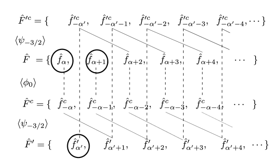
Figure 5: An example of Type-I $p=3/2>q=1/2$ for the three massless generation case in Eq. (19): a massless mode $\hat{f}_{0}$ is realized by certain linear combinations of the components $\hat{f}_{\alpha+3k}$ and $\hat{f}^{\prime}_{\alpha^{\prime}+1+3k}$ $(k=1,2,\cdots)$, and the constructional element of the massless mode is determined by its mixing coefficients $U_{0,3k}^{f}$ and $U_{0,3k+1}^{f\prime}$ given in Eqs. (22), (23) and (24); and etc., where a main element of each massless chiral mode is surround by a circle, and the components of the matter fields $\hat{F}$, $\hat{F}^{c}$, $\hat{F}^{\prime}$ and $\hat{F}^{\prime c}$ connected by solid and dashed lines have a mass term that comes from the VEVs $\langle\psi_{-3/2}\rangle$ and $\langle\phi_{0}\rangle$, respectively, and the mass term of the solid line that comes from the VEV $\langle\psi_{-3/2}\rangle$ dominantly contributes to whether massless modes appear or not.

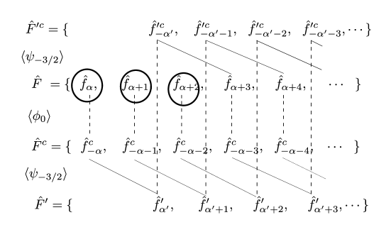
Figure 6: An example of Type-II $p=q=3/2$ for the three massless generation case in Eq. (19): each massless mode $\hat{f}_{n}$ is realized by a certain linear combination of the components $\hat{f}_{\alpha+3k+n}$ and $\hat{f}^{\prime}_{\alpha^{\prime}+3k+n}$ $(k=1,2,\cdots)$, and the constructional element of its massless mode is determined by its mixing coefficients $U_{n,3k+n}^{f}$ and $U_{n,3k+n}^{f\prime}$ given in Eqs. (22), (23) and (25), where the explanation of the circle and lines is given in Fig. 5.

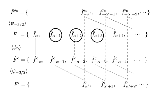
Figure 7: An example of Type-III $p=3/2<q=5/2$ for the three massless generation case in Eq. (19): each massless mode $\hat{f}_{n}$ is realized by a certain linear combination of the components $\hat{f}_{\alpha+3k+n+1}$ and $\hat{f}^{\prime}_{\alpha^{\prime}+3k+n}$ $(k=1,2,\cdots)$, and the constructional element of its massless mode is determined by its mixing coefficients $U_{n,3k+n+1}^{f}$ and $U_{n,3k+n}^{f\prime}$ given in Eqs. (22), (23) and (26), where the explanation of the circle and lines is given in Fig. 5.

To clarify the meaning of the above mixing coefficients and the relation between their initial conditions, we give examples of Type-I $p=3/2>q=1/2$, Type-II $p=q=3/2$ and Type-III $p=3/2<q=5/2$ for the three massless generation case in Eq. (19). First, for $p=3/2$ and $q=1/2$ from Fig. 5, we find that the components $\hat{f}_{\alpha}$ and $\hat{f}_{\alpha+1}$ of the matter field $\hat{F}$ and the component $\hat{f}^{\prime}_{\alpha^{\prime}}$ of the matter field $\hat{F}^{\prime}$ are a main element of massless modes $\hat{f}_{0}$, $\hat{f}_{1}$ and $\hat{f}_{2}$, respectively; a massless mode $\hat{f}_{0}$ is realized by a certain linear combination of the components $\hat{f}_{\alpha+3k}$ and $\hat{f}^{\prime}_{\alpha^{\prime}+1+3k}$ $(k=1,2,\cdots)$, and the constructional element of the massless mode is determined by its mixing coefficients $U_{0,3k}^{f}$ and $U_{0,3k+1}^{f\prime}$ given in Eqs. (22), (23) and (24); another massless mode $\hat{f}_{1}$ is realized by a certain linear combination of the components $\hat{f}_{\alpha+3k+1}$ and $\hat{f}^{\prime}_{\alpha^{\prime}+2+3k}$, and the element of the massless mode is determined by its mixing coefficients $U_{1,3k+1}^{f}$ and $U_{1,3k+2}^{f\prime}$; and the other massless mode $\hat{f}_{2}$ is realized by a certain linear combination of the components $\hat{f}^{\prime}_{\alpha^{\prime}+3k}$ and $\hat{f}_{\alpha+3k+2}$, and the element of the massless mode is determined by its mixing coefficients $U_{2,3k}^{f\prime}$ and $U_{2,3k+2}^{f}$. Next, for $p=q=3/2$ from Fig. 6, we find that each component $\hat{f}_{\alpha+n}$ $(n=0,1,2)$ of the matter field $\hat{F}$ is a main element of each massless mode $\hat{f}_{n}$; each massless mode $\hat{f}_{n}$ is realized by a certain linear combination of the components $\hat{f}_{\alpha+3k+n}$ and $\hat{f}^{\prime}_{\alpha^{\prime}+3k+n}$ $(k=1,2,\cdots)$, and the constructional element of its massless mode is determined by its mixing coefficients $U_{n,3k+n}^{f}$ and $U_{n,3k+n}^{f\prime}$ given in Eqs. (22), (23) and (25). Finally, for $p=3/2$ and $q=5/2$ from Fig. 7, we find that each component $\hat{f}_{\alpha+n+1}$ of the matter field $\hat{F}$ is a main element of each massless mode $\hat{f}_{n}$; each massless mode $\hat{f}_{n}$ is realized by a certain linear combination of the components $\hat{f}_{\alpha+3k+n+1}$ and $\hat{f}^{\prime}_{\alpha^{\prime}+3k+n}$ $(k=1,2,\cdots)$, and the constructional element of its massless mode is determined by its mixing coefficients $U_{n,3k+n+1}^{f}$ and $U_{n,3k+n}^{f\prime}$ given in Eqs. (22), (23) and (26). Since the isolated components $\hat{f}_{\alpha}$ and $\hat{f}_{-\alpha}^{c}$ have only a mass term from the VEV $\langle\phi_{0}\rangle$, they are massive.

Regardless of these three types of conditions, the $2p$ massless modes $f_{n}$ $(n=0,1,\cdots 2p-1)$ can arise at low energy because the initial value of $U_{n,\ell}^{f}$ or $U_{n,\ell^{\prime}}^{f\prime}$ determines $U_{n,i}^{f}$ and $U_{n,j}^{f\prime}$ completely. For $p=1/2,3/2,5/2,\cdots,S^{\prime}$, we can get $1,3,5,\cdots,2S^{\prime}$ chiral generations. This means that only odd number generations are allowed. Especially, if $S^{\prime}=3/2$ only one or three generations are allowed.

The remaining task is to verify the normalizable condition of the mixing coefficients $U_{n,i}^{f}$ and $U_{n,j}^{f\prime}$. Any massless mode $\hat{f}_{n}$ $(n=0,1,2,\cdots,2p-1)$ must satisfy the normalization conditions $\sum_{s=0}^{\infty}U_{n,\ell+2ps}^{f}<\infty$ and $\sum_{s=0}^{\infty}U_{n,\ell^{\prime}+2ps}^{f\prime}<\infty$. This requirement leads to the conditions

$$\lim_{i\to\infty}\left|\frac{U_{n,i+2p}^{f}}{U_{n,i}^{f}}\right|<1\ \ \ \mbox{and}\ \ \ \lim_{i\to\infty}\left|\frac{U_{n,i+2p}^{f\prime}}{U_{n,i}^{f\prime}}\right|<1.$$ (27)

As we discussed before, by using the asymptotic behavior of the CGC $D_{i,j}^{\alpha,\beta,S}\sim i^{S}$ given by Eq. (4), for $S<S^{\prime}$, $\sum_{s=0}^{\infty}|U_{n,\ell+2ps}^{f}|^{2}$ and $\sum_{s=0}^{\infty}|U_{n,\ell^{\prime}+2ps}^{f\prime}|^{2}$ converge, and then these massless particles appear at low energy; For $S>S^{\prime}$, $\sum_{k=0}^{\infty}|U_{n,\ell+2pk}^{f}|^{2}$ and $\sum_{s=0}^{\infty}|U_{n,\ell^{\prime}+2ps}^{f\prime}|^{2}$ diverge, and the massless ones do not emerge at low energy. This setup cannot satisfy the marginal assignment $S=S^{\prime}$ because any integer $S$ is not equal to the half-integer $S^{\prime}$. We take a phase convention for the massless modes $f_{n}$ so that each larger initial mixing coefficient is real and positive.

4 Structures of Yukawa Coupling Constants

Let us investigate structures of Yukawa coupling constants governed by the horizontal symmetry $SU(1,1)$. We first introduce three matter fields $\hat{F}$ and $\hat{G}$ with the lowest weight $+\alpha$ and $+\beta$, and $\hat{H}$ with the highest weight $-\gamma$, where these weights must satisfy a weight condition $\Delta:=\gamma-\alpha-\beta$, and $\Delta$ is a non-negative integer number. Here we consider a Yukawa coupling superpotential term

$$W_{\rm Yukawa}=y\hat{F}\hat{G}\hat{H},$$ (28)

where $y$ is a dimensionless coupling constant. We suppose that the matter fields $\hat{F}$ and $\hat{G}$ include three generations and the matter field $\hat{H}$ includes only one generation, and the mixing coefficient forms are given by

$$\hat{f}_{\alpha+i}=\sum_{m=0}^{2}\hat{f}_{m}U_{m,i}^{f}+[\cdots],\ \ \ \hat{g}_{\beta+i}=\sum_{m=0}^{2}\hat{g}_{m}U_{m,i}^{g}+[\cdots],\ \ \ \hat{h}_{-\gamma-i}=\hat{h}U_{i}^{h}+[\cdots],$$ (29)

where $m=0,1,2$, and $[\cdots]$ represents the corresponding massive modes. The explicit expressions for the mixing coefficients $U_{m,i}^{f}$, $U_{m,i}^{g}$ and $U_{i}^{h}$ are determined by the mechanism of the spontaneous generation of generations as we have discussed in §3. Since the multiplets $\hat{F},\hat{G}$ and $\hat{H}$ are unitary representations of $SU(1,1)$, all coefficients $U$ should be row vectors in unitary matrices, and then they satisfy $\sum_{i=0}^{\infty}U_{m,i}^{f*}U_{n,i}^{f}=\delta_{mn}$ and so on.

The Yukawa coupling constants of the massless mode $\hat{h}$ coupling to $\hat{f}_{n}$ and $\hat{g}_{n}$ are derived by extracting the massless modes from the term in Eq. (28)

$$W_{\rm Yukawa}=\sum_{m,n=0}^{2}y^{mn}\hat{f}_{m}\hat{g}_{n}\hat{h},$$ (30)

where $y^{mn}$ are the coupling constants. By using the CGC in Eq. (6), the coupling matrix $y^{mn}$ is given by

$$y^{mn}=y\sum_{i,j=0}^{\infty}C_{i,j}^{\alpha,\beta,\Delta}U_{m,i}^{f}U_{n,j}^{g}U_{i+j-\Delta}^{h},$$ (31)

where the mixing coefficients $U^{f,g}_{m,i}$ and $U_{i}^{h}$ are determined by the $SU(1,1)$ CGCs, the VEVs of structure fields, and the corresponding coupling constants as we discussed in the previous section.

In the rest of this section, we first review the structures of the Yukawa couplings derived from the mixing coefficients of two structure fields with an integer spin, which is discussed in Ref. [23, 18]. We discuss the Yukawa coupling structures determined by the mixing coefficients of one structure field with an integer spin and one with a half-integer spin.

4.1 Two Structure Fields with an Integer Spin

Let us examine the structures of Yukawa couplings given by the form of the mixing coefficients in Eq. (11) from two structure fields with integer spins as in Fig. 3. In this case, the mixing coefficients are given by

$$U^{f}_{n,i}=U^{f}_{n}\sum_{s=0}^{\infty}\delta_{j,n+3s}(-\epsilon_{F})^{s}b^{f}_{m,s},\ \ \epsilon_{F}=\frac{x_{F}\langle\psi_{F0}\rangle}{x_{F}^{\prime}\langle\psi_{F-3}^{\prime}\rangle},\ \ b_{n,s}^{f}=\prod_{r=0}^{s-1}\frac{D^{\alpha,\alpha,S_{F}}_{3r+n,3r+n}}{D^{\alpha,\alpha,S_{F}^{\prime}}_{3r+n,3(r+1)+n}},$$ (32)

$$U^{g}_{n,i}=U^{g}_{n}\sum_{s=0}^{\infty}\delta_{i,n+3s}(-\epsilon_{G})^{s}b^{g}_{m,s},\ \ \epsilon_{G}=\frac{x_{G}\langle\psi_{G0}\rangle}{x_{G}^{\prime}\langle\psi_{G-3}^{\prime}\rangle},\ \ b_{n,s}^{g}=\prod_{r=0}^{s-1}\frac{D^{\beta,\beta,S_{G}}_{3r+n,3r+n}}{D^{\beta,\beta,S_{G}^{\prime}}_{3r+n,3(r+1)+n}},$$ (33)

$$U_{i}^{h}=U_{0}^{h}(-\epsilon_{H})^{i}b_{i}^{h},\ \ \epsilon_{H}=\frac{x_{H}\langle\psi_{H0}\rangle}{x_{H}^{\prime}\langle\psi_{H+1}^{\prime}\rangle},\ \ b_{i}^{h}=\prod_{r=0}^{i-1}\frac{D^{\gamma,\gamma,S_{H}}_{r,r}}{D^{\gamma,\gamma,S_{H}^{\prime}}_{r,r+1}},$$ (34)

where the subscripts $F,G,H$ and the superscripts $f,g,h$ represent the matter fields $\hat{F},\hat{G},\hat{H}$. From the mixing coefficients in Eqs. (32)-(34), the Yukawa coupling in Eq. (31) is in the form

$$y^{mn}=yU^{f}_{m}U^{g}_{n}U_{0}^{h}\sum_{r,s=0}^{\infty}(\epsilon_{F}\epsilon_{H}^{3})^{r}(\epsilon_{G}\epsilon_{H}^{3})^{s}(-\epsilon_{H})^{m+n-\Delta}C_{m+3r,n+3s}^{\alpha,\beta,\Delta}b^{f}_{m,r}b^{g}_{n,s}b^{h}_{m+n-\Delta+3(r+s)},$$ (35)

where $\Delta:=\gamma-\alpha-\beta$.

We consider the contribution of the nonzero $s$ and/or $r$ terms for the Yukawa coupling in Eq. (35). The asymptotic behavior of $D_{j,i}^{\beta,\alpha,S}$ for the large $S$ limit with $|i-j|$ fixed,

$$D_{j,i}^{\beta,\alpha,S}\simeq(-i)^{i}S^{i+j+\alpha+\beta-1}\frac{1}{\sqrt{i!j!\Gamma(2\alpha+i)\Gamma(2\beta+j)}},$$ (36)

leads to

$$b_{n,s}^{f}\simeq\prod_{r=0}^{s-1}\frac{(S_{F})^{6r+2n+2\alpha-1}}{(S_{F}^{\prime})^{6r+2n+2\alpha+2}}\sqrt{\frac{(3r+n+3)!\Gamma(2\alpha+3r+n+3)}{(3r+n)!\Gamma(2\alpha+3r+n)}},$$

$$b_{i}^{h}\simeq\prod_{r=0}^{i-1}\frac{(S_{H})^{2r+2\gamma-1}}{(S_{H}^{\prime})^{2r+2\gamma}}\sqrt{(r+1)(2\gamma+r)},$$ (37)

where $b_{n,s}^{g}$ is given by replacing $F$ and $\alpha$ in $b_{n,s}^{f}$ by $G$ and $\beta$. Note that we only consider the cases with $S_{F}\leq S_{F}^{\prime}$, $S_{G}\leq S_{G}^{\prime}$ and $S_{H}\leq S_{H}^{\prime}$ because each massless mode is absent in the cases with $S_{F}>S_{F}^{\prime}$, $S_{G}>S_{G}^{\prime}$, and $S_{H}>S_{H}^{\prime}$, and there are no Yukawa couplings between massless modes. The $b_{n,s}^{f}$ quickly decreases as the $SU(1,1)$ spin becomes large, so the contribution from the nonzero $s$ and/or $r$ terms is negligible. Next we consider cases with smaller $SU(1,1)$ spins, where $S_{F}^{\prime}$ and $S_{G}^{\prime}$ must be larger than or equal to three, and $S_{H}^{\prime}$ must be larger than or equal to one due to the existence of the nonvanishing VEVs of the structure fields. For $S_{F}<S_{F}^{\prime}$, $S_{G}<S_{G}^{\prime}$ and $S_{H}<S_{H}^{\prime}$, typical weights $\alpha$, $\beta$ and $\gamma$ give $b_{n,0}^{f}\gg b_{n,1}^{f}\gg\cdots$, $b_{n,0}^{g}\gg b_{n,1}^{g}\gg\cdots$ and $b_{n}^{h}\gg b_{n+3}^{h}\gg\cdots$, respectively. Thus, even if $|\epsilon_{F}|$ and $|\epsilon_{G}|\simeq 1$, the contribution of the terms $(r+s>0)$ in Eq. (35) is negligible. For $S_{F}=S_{F}^{\prime}$, $S_{G}=S_{G}^{\prime}$ and $S_{H}=S_{H}^{\prime}$, $b_{n,0}^{f}\simeq b_{n,1}^{f}\simeq\cdots$, $b_{n,0}^{g}\simeq b_{n,1}^{g}\simeq\cdots$ and $b_{n}^{h}\simeq b_{n+3}^{h}\simeq\cdots$, respectively, but $C_{i,j}^{\alpha,\beta,\Delta}>C_{i+3,j}^{\alpha,\beta,\Delta}\simeq C_{i,j+3}^{\alpha,\beta,\Delta}>C_{i+3,j+3}^{\alpha,\beta,\Delta}>\cdots$ and the parameters $\epsilon$ must satisfy the relations $\epsilon_{F,G}<\epsilon_{F,Gcr}^{g=3}$ and $\epsilon_{H}<\epsilon_{Hcr}^{g=1}$ to produce each corresponding massless mode, where $\left.1/\sqrt{20}\right|_{S_{F,G}=S_{F,G}^{\prime}=3}\leq\epsilon_{F,Gcr}^{g=3}<\left.1\right|_{S_{F,G}=S_{F,G}^{\prime}\to\infty}$ and $\left.1/\sqrt{2}\right|_{S_{H}=S_{H}^{\prime}=1}\leq\epsilon_{Hcr}^{g=1}<\left.1\right|_{S_{H}=S_{H}^{\prime}\to\infty}$ from Eq. (14). Thus, we can neglect the contributions from the nonzero $s$ and/or $r$ terms in Eq. (35) as long as the corresponding $s=r=0$ term exists. That is we can use the mixing coefficients of three generations in Fig. 1 instead of the ones in Fig. 3. When $\Delta>0$, some matrix elements have no contribution from the $s=r=0$ term. For example, for $\Delta=1$, the $(r,s)=0$ term of $y^{00}$ is not allowed and the $(r,s)=(1,0),(0,1)$ terms dominantly contribute to this matrix. In the following discussion, we analyze Yukawa matrices for the $s=r=0$ term in Eq. (35)

$$y^{mn}=yU_{m}^{f}U_{n}^{g}U_{0}^{h}(-\epsilon_{H})^{m+n-\Delta}C_{m,n}^{\alpha,\beta,\Delta}b^{h}_{m+n-\Delta}.$$ (38)

Let us examine this structure for large $SU(1,1)$ spin $S_{H}^{\prime}$. In this case, since $b_{i}^{h}\simeq 0$ for $(i\geq 1)$, $U^{h}_{i}\simeq\delta_{i,0}$. Thus, the massless mode $\hat{h}$ emerges as the pure $0$th component of $\hat{h}_{-\gamma-i}$. For $\Delta\geq 0$, the Yukawa coupling matrix is $y^{mn}=yC_{m,n}^{\alpha,\beta,\Delta}\delta_{m+n-\Delta,0}$. For $\Delta=0,4$, the rank of this matrix is one, and only one generation of each of $\hat{f}_{m}$ and $\hat{g}_{n}$ has a mass when $\hat{h}$ has a nonvanishing VEV. For $\Delta=1,3$, the rank of this matrix is two, and two generations of $\hat{f}_{m}$ and $\hat{g}_{n}$ have degenerate masses. For $\Delta=2$, the rank of this matrix is three, and three generations of $\hat{f}_{m}$ and $\hat{g}_{n}$ have almost degenerate masses. For $\Delta\geq 5$, there is no Yukawa coupling.

Let us begin to analyze the structure of the Yukawa couplings in Eq. (38) for small $S_{H}^{\prime}$. We here concentrate our discussion on the $\Delta=0$ case. To examine this pattern, it is convenient to introduce the normalized matrix $\tilde{y}^{mn}:=y^{mn}/y^{00}$. By using the CGC in Eq. (6), the normalized matrix $\tilde{y}^{mn}$ is given by

$$\tilde{y}^{mn}:=\frac{y^{mn}}{y^{00}}=\tilde{U}_{m}^{f}\tilde{U}_{n}^{g}\epsilon_{H}^{m+n}\sqrt{\frac{(m+n)!}{m!n!}\frac{\Gamma(2\gamma)\Gamma(2\alpha+m)\Gamma(2\beta+n)}{\Gamma(2\gamma+m+n)\Gamma(2\alpha)\Gamma(2\beta)}}\ b_{m+n}^{h},$$ (39)

where $b^{h}_{0}=1$, $\tilde{U}^{f}_{m}:=U^{f}_{m}/U^{f}_{0}$, and $\tilde{U}^{g}_{n}:=U^{g}_{n}/U^{g}_{0}$. The explicit form is

$$\tilde{y}^{mn}=\left(\begin{array}[]{lll}1&\tilde{U}_{1}^{g}\epsilon_{H}\sqrt{\frac{\beta}{\gamma}}b^{h}_{1}&\tilde{U}_{2}^{g}\epsilon_{H}^{2}\sqrt{\frac{(2\beta+1)\beta}{(2\gamma+1)\gamma}}b^{h}_{2}\\ \tilde{U}_{1}^{f}\epsilon_{H}\sqrt{\frac{\alpha}{\gamma}}b^{h}_{1}&\tilde{U}_{1}^{f}\tilde{U}_{1}^{g}\epsilon^{2}_{H}\sqrt{\frac{4\alpha\beta}{(2\gamma+1)\gamma}}b^{h}_{2}&\tilde{U}_{1}^{f}\tilde{U}_{2}^{g}\epsilon_{H}^{3}\sqrt{\frac{3(2\beta+1)\alpha\beta}{\gamma(\gamma+1)(2\gamma+1)}}b^{h}_{3}\\ \tilde{U}_{2}^{f}\epsilon_{H}^{2}\sqrt{\frac{(2\alpha+1)\alpha}{(2\gamma+1)\gamma}}b^{h}_{2}&\tilde{U}_{2}^{f}\tilde{U}_{1}^{g}\epsilon_{H}^{3}\sqrt{\frac{3(2\alpha+1)\alpha\beta}{\gamma(\gamma+1)(2\gamma+1)}}b^{h}_{3}&\tilde{U}_{2}^{f}\tilde{U}_{2}^{g}\epsilon_{H}^{4}\sqrt{\frac{6(2\alpha+1)(2\beta+1)\alpha\beta}{\gamma(\gamma+1)(2\gamma+1)(2\gamma+3)}}b^{h}_{4}\end{array}\right).$$ (43)

This matrix is diagonalized by a bi-unitary transformation because it is a complex matrix:

$$V^{\dagger}\tilde{y}^{mn}U=\mbox{diag}(\tilde{y}_{0},\tilde{y}_{1},\tilde{y}_{2}),$$ (44)

where $V$ and $U$ are unitary matrices.

To understand the features of the Yukawa coupling matrix in Eq. (39), we expand the eigenvalues $\tilde{y}_{0},\tilde{y}_{1}$,$\tilde{y}_{2}$ of this type of matrix in a power series in $\epsilon_{H}^{2}$ by $\tilde{y}_{0}=w_{0}+O(\epsilon_{H}^{2})$, $\tilde{y}_{1}=\epsilon^{2}w_{1}+O(\epsilon_{H}^{4})$, and $\tilde{y}_{2}=\epsilon^{4}w_{2}+O(\epsilon_{H}^{6})$. The leading terms have the expressions $w_{0}=\tilde{y}^{00}$, $\epsilon^{2}w_{1}=\mbox{det}(\tilde{y}^{mn})_{2\times 2}/\tilde{y}^{00}$, and $\epsilon^{4}w_{2}=\mbox{det}(\tilde{y}^{mn})_{3\times 3}/\mbox{det}(\tilde{y}^{mn})_{2\times 2}$, where $\mbox{det}(\tilde{y}^{mn})_{2\times 2}:=\tilde{y}^{00}\tilde{y}^{11}-\tilde{y}^{01}\tilde{y}^{10}$, and $\mbox{det}(\tilde{y}^{mn})_{3\times 3}:=\tilde{y}^{22}(\tilde{y}^{00}\tilde{y}^{11}-\tilde{y}^{01}\tilde{y}^{10})-\tilde{y}^{21}(\tilde{y}^{00}\tilde{y}^{12}-\tilde{y}^{10}\tilde{y}^{02})-\tilde{y}^{20}(\tilde{y}^{11}\tilde{y}^{02}-\tilde{y}^{01}\tilde{y}^{12})$. The straightforward calculation gives the expressions of $\tilde{y}_{0},\tilde{y}_{1},\tilde{y}_{2}$ in the forms

$$\tilde{y}_{0}=1+O(\epsilon_{H}^{2}),$$

$$\tilde{y}_{1}=\epsilon_{H}^{2}\sqrt{\frac{\alpha\beta}{(2\gamma+1)\gamma}}\tilde{U}^{f}_{1}\tilde{U}^{g}_{1}\ X_{\gamma}+O(\epsilon_{H}^{4}),$$

$$\tilde{y}_{2}=\epsilon_{H}^{4}\sqrt{\frac{6\alpha\beta(2\alpha+1)(2\beta+1)}{\gamma(\gamma+1)(2\gamma+1)(2\gamma+3)}}\tilde{U}^{f}_{2}\tilde{U}^{g}_{2}\ \frac{Z_{\gamma}}{X_{\gamma}}+O(\epsilon_{H}^{6}),$$ (45)

where the $X_{\gamma}$ and $Z_{\gamma}$ only depend on the representations of $SU(1,1)$:

$$X_{\gamma}:= 2b_{2}^{h}-b_{1}^{h2}\sqrt{\frac{2\gamma+1}{\gamma}},$$ (46)

$$Z_{\gamma}:= 2b_{2}^{h}b_{4}^{h}+2b_{1}^{h}b_{2}^{h}b_{3}^{h}\sqrt{\frac{2\gamma+3}{2\gamma}}-3b_{3}^{h2}\sqrt{\frac{2\gamma+3}{6(\gamma+1)}}$$

$$-2b_{2}^{h3}\sqrt{\frac{(\gamma+1)(2\gamma+3)}{6\gamma(2\gamma+1)}}-b_{1}^{h2}b_{4}^{h}\sqrt{\frac{2\gamma+1}{\gamma}}.$$ (47)

In this case, the unitary matrices $U$ and $V$ are approximately expressed by

$$U\simeq\left(\begin{array}[]{ccc}1&-\epsilon_{H}\tilde{U}^{g}_{1}\sqrt{\frac{\beta}{\gamma}}b^{h}_{1}&-\epsilon_{H}^{2}\tilde{U}^{g}_{2}\frac{\sqrt{\frac{4\beta(2\beta+1)}{2\gamma+1}}b^{h2}_{2}-\sqrt{\frac{3\beta(2\beta+1)}{\gamma+1}}b^{h}_{1}b^{h}_{3}}{2\sqrt{\gamma}b^{h}_{2}-\sqrt{2\gamma+1}b^{h2}_{1}}\\ \epsilon_{H}\tilde{U}^{g}_{1}\sqrt{\frac{\beta}{\gamma}}b^{h}_{1}&1&-\epsilon_{H}\frac{\tilde{U}^{g}_{2}}{\tilde{U}^{g}_{1}}\frac{\sqrt{\frac{3(2\beta+1)\gamma}{\gamma+1}}b^{h}_{3}-\sqrt{2\beta+1}b^{h}_{1}b^{h}_{2}}{2\sqrt{\gamma}b^{h}_{2}-\sqrt{2\gamma+1}b^{h2}_{1}}\\ \epsilon_{H}^{2}\tilde{U}^{g}_{2}\sqrt{\frac{(2\beta+1)\beta}{(2\gamma+1)\gamma}}b^{h}_{2}&\epsilon_{H}\frac{\tilde{U}^{g}_{2}}{\tilde{U}^{g}_{1}}\frac{\sqrt{\frac{3(2\beta+1)\gamma}{\gamma+1}}b^{h}_{3}-\sqrt{2\beta+1}b^{h}_{1}b^{h}_{2}}{2\sqrt{\gamma}b^{h}_{2}-\sqrt{2\gamma+1}b^{h2}_{1}}&1\\ \end{array}\right),$$ (51)

(52)

$$V\simeq\left(\begin{array}[]{ccc}1&-\epsilon_{H}\tilde{U}^{f}_{1}\sqrt{\frac{\alpha}{\gamma}}b^{h}_{1}&-\epsilon_{H}^{2}\tilde{U}^{f}_{2}\frac{\sqrt{\frac{4\alpha(2\alpha+1)}{2\gamma+1}}b^{h2}_{2}-\sqrt{\frac{3\alpha(2\alpha+1)}{\gamma+1}}b^{h}_{1}b^{h}_{3}}{2\sqrt{\gamma}b^{h}_{2}-\sqrt{2\gamma+1}b^{h2}_{1}}\\ \epsilon_{H}\tilde{U}^{f}_{1}\sqrt{\frac{\alpha}{\gamma}}b^{h}_{1}&1&-\epsilon_{H}\frac{\tilde{U}^{f}_{2}}{\tilde{U}^{f}_{1}}\frac{\sqrt{\frac{3(2\alpha+1)\gamma}{\gamma+1}}b^{h}_{3}-\sqrt{2\alpha+1}b^{h}_{1}b^{h}_{2}}{2\sqrt{\gamma}b^{h}_{2}-\sqrt{2\gamma+1}b^{h2}_{1}}\\ \epsilon_{H}^{2}\tilde{U}^{f}_{2}\sqrt{\frac{(2\alpha+1)\alpha}{(2\gamma+1)\gamma}}b^{h}_{2}&\epsilon_{H}\frac{\tilde{U}^{f}_{2}}{\tilde{U}^{f}_{1}}\frac{\sqrt{\frac{3(2\alpha+1)\gamma}{\gamma+1}}b^{h}_{3}-\sqrt{2\alpha+1}b^{h}_{1}b^{h}_{2}}{2\sqrt{\gamma}b^{h}_{2}-\sqrt{2\gamma+1}b^{h2}_{1}}&1\\ \end{array}\right).$$ (56)

To understand the hierarchical pattern, it is useful to see some examples. A set of $SU(1,1)$ spins $(S_{H},S_{H}^{\prime})=(0,1)$ determines the $b_{i}^{h}$ in Eq. (34) given by

$$b_{i}^{h}=\sqrt{\frac{\Gamma(2\gamma)}{2^{i}i!\Gamma(2\gamma+i)}}.$$ (58)

This leads to

$$\tilde{y}_{0}=1+O(\epsilon_{H}^{2}),$$

$$\tilde{y}_{1}=-\epsilon_{H}^{2}\frac{\sqrt{\alpha\beta}}{2\gamma^{2}(2\gamma+1)}+O(\epsilon_{H}^{4}),$$

$$\tilde{y}_{2}=\epsilon_{H}^{4}\frac{\sqrt{\alpha\beta(2\alpha+1)(2\beta+1)}}{4\gamma^{3}(\gamma+1)^{2}(2\gamma+1)^{2}(2\gamma+3)}+O(\epsilon_{H}^{6}).$$ (59)

We can easily calculate the eigenvalues for some weight sets: For the weight set $\alpha=\beta=\gamma/2=1/2$, $\tilde{y}_{0}=1+O(\epsilon_{H}^{2})$, $\tilde{y}_{1}=-\epsilon_{H}^{2}/12+O(\epsilon_{H}^{4})$, and $\tilde{y}_{2}=\epsilon_{H}^{4}/720+O(\epsilon_{H}^{6})$. For $\alpha=\beta=\gamma/2=1$, $\tilde{y}_{0}=1+O(\epsilon_{H}^{2})$, $\tilde{y}_{1}=-\epsilon_{H}^{2}/40+O(\epsilon_{H}^{4})$, and $\tilde{y}_{2}=\epsilon_{H}^{4}/16800+O(\epsilon_{H}^{6})$. For $\alpha=\beta=\gamma/2=2$, $\tilde{y}_{0}=1+O(\epsilon_{H}^{2})$, $\tilde{y}_{1}=-\epsilon_{H}^{2}/144+O(\epsilon_{H}^{4})$, and $\tilde{y}_{2}=\epsilon_{H}^{4}/570240+O(\epsilon_{H}^{6})$. For $\alpha=\beta=\gamma/2\to\infty$, $\tilde{y}_{0}\simeq 1$, $\tilde{y}_{1}\simeq 0$, and $\tilde{y}_{2}\simeq 0$. Another set of $SU(1,1)$ spins $(S_{H},S_{H}^{\prime})=(1,1)$ provides the $b_{i}^{h}$ given by

$$b_{i}^{h}=\sqrt{\frac{2^{i}\Gamma(2\gamma)}{i!\Gamma(2\gamma+i)}}\frac{\Gamma(\gamma+i)}{\Gamma(\gamma)}$$ (60)

and this gives

$$\tilde{y}_{0}=1+O(\epsilon_{H}^{2}),$$

$$\tilde{y}_{1}=-\epsilon_{H}^{2}\frac{\sqrt{\alpha\beta}}{2(2\gamma+1)}+O(\epsilon_{H}^{4}),$$

$$\tilde{y}_{2}=\epsilon_{H}^{4}\frac{\gamma\sqrt{\alpha\beta(2\alpha+1)(2\beta+1)}}{4(2\gamma+1)^{2}(2\gamma+3)}+O(\epsilon_{H}^{6}).$$ (61)

We also give the eigenvalues for some weight sets: For the weight set $\alpha=\beta=\gamma/2=1/2$, $\tilde{y}_{0}=1+O(\epsilon_{H}^{2})$, $\tilde{y}_{1}=\epsilon_{H}^{2}/12+O(\epsilon_{H}^{4})$, and $\tilde{y}_{2}=\epsilon_{H}^{4}/180+O(\epsilon_{H}^{6})$. For $\alpha=\beta=\gamma/2=1$, $\tilde{y}_{0}=1+O(\epsilon_{H}^{2})$, $\tilde{y}_{1}=\epsilon_{H}^{2}/10+O(\epsilon_{H}^{4})$, and $\tilde{y}_{2}=3\epsilon_{H}^{4}/700+O(\epsilon_{H}^{6})$. For $\alpha=\beta=\gamma/2=2$, $\tilde{y}_{0}=1+O(\epsilon_{H}^{2})$, $\tilde{y}_{1}=\epsilon_{H}^{2}/9+O(\epsilon_{H}^{4})$, and $\tilde{y}_{2}=10\epsilon_{H}^{4}/891+O(\epsilon_{H}^{6})$. For $\alpha=\beta=\gamma/2\to\infty$, $\tilde{y}_{0}=1+O(\epsilon_{H}^{2})$, $\tilde{y}_{1}=\epsilon_{H}^{2}/8+O(\epsilon_{H}^{4})$, and $\tilde{y}_{2}=\epsilon_{H}^{4}/64+O(\epsilon_{H}^{6})$. From the above, we determine that for the marginal assignment $(S_{H}=S_{H}^{\prime})$ the eigenvalues of the Yukawa coupling constants are relatively stable with respect to changing the weights, but for the other assignments $(S_{H}<S_{H}^{\prime})$ they are very sensitive.

We now summarize the results of this part. For $S_{H}<S_{H}^{\prime}$, as the weight $\gamma$ increases, the eigenvalues $\tilde{y}_{1}$ and $\tilde{y}_{2}$ decrease. For $\gamma\to\infty$, $\tilde{y}_{1}$ and $\tilde{y}_{2}$ become zero. For the marginal assignment $S_{H}=S_{H}^{\prime}$, $\tilde{y}_{1}$ and $\tilde{y}_{2}$ become certain non-zero values, which depend on the value of the $SU(1,1)$ spin and the weights $\alpha$ and $\beta$. Even in this case, for large $SU(1,1)$ spin $S_{H}(=S_{H}^{\prime})$, $y_{1}$ and $y_{2}$ become zero. The mass parameters at the GUT scale in the MSSM are given by Ref. [24] for several values of $\tan\beta$ by using the renormalization group equations of the two-loop gauge couplings and the two-loop Yukawa couplings assuming an effective SUSY scale of 500 GeV. Translating these mass parameters for $\tan\beta=10$ into coupling constants, the constants for the up-type quark, the down-type quark, and the charged lepton are $(\tilde{y}_{0},\tilde{y}_{1},\tilde{y}_{2})\simeq(1,2.5\times 10^{-3},6.7\times 10^{-6})$, $(1,2\times 10^{-2},1.0\times 10^{-3})$, and $(1,6\times 10^{-2},2.5\times 10^{-4})$, respectively, and the values are almost the same for $\tan\beta=38$ and $50$. When we take the value of the $\epsilon_{H}$ to range from $0.1$ to $1$, small $SU(1,1)$ spins are preferred and small $SU(1,1)$ weights are also preferred except for the marginal assignment.

In this paper, we will not discuss the CKM [25, 26] and MNS matrices [27] because these matrices are very dependent on the choice of the weights and spins of $SU(1,1)$, where of course we need to set up the neutrino sector. Some discussions of the CKM and the MNS matrices in this model can be found in Ref. [23] and [28], respectively.

4.2 One Structure Field with an Integer Spin and One with a Half-Integer Spin

We introduce additional matter fields $\hat{F}^{\prime}$ and $\hat{G}^{\prime}$ with the lowest weights $\alpha^{\prime}$ and $\beta^{\prime}$ and $\hat{H}^{\prime}$ with the highest weight $-\gamma^{\prime}$, which have the same representations as the matter fields $\hat{F}$, $\hat{G}$, $\hat{H}$ except that of $SU(1,1)$, respectively. In this case, some weight conditions allow not only one Yukawa coupling superpotential term but also another. This corresponds to the extended higgs sector discussed in Ref. [18]. One of the main aims of this paper is to show the effects of the structure fields with half-integer spins of $SU(1,1)$. Thus, in this paper we will not discuss the multi-Yukawa coupling constants and we only discuss some examples of the structures of each Yukawa coupling constant.

We suppose that the matter fields $\hat{F}+\hat{F}^{\prime}$ and $\hat{G}+\hat{G}^{\prime}$ include three generations and the matter fields $\hat{H}+\hat{H}^{\prime}$ include only one generation and the following mixing coefficient forms are

$$\hat{f}_{\alpha+i}=\sum_{m=0}^{2}\hat{f}_{m}U_{m,i}^{f}+[\cdots],\ \ \ \hat{g}_{\beta+i}=\sum_{m=0}^{2}\hat{g}_{m}U_{m,i}^{g}+[\cdots],\ \ \ \hat{h}_{-\gamma-i}=\hat{h}U_{i}^{h}+[\cdots],$$

$$\hat{f}_{\alpha^{\prime}+i}^{\prime}=\sum_{m=0}^{2}\hat{f}_{m}^{\prime}U_{m,i}^{f\prime}+[\cdots],\ \ \ \hat{g}_{\beta^{\prime}+i}^{\prime}=\sum_{m=0}^{2}\hat{g}_{m}^{\prime}U_{m,i}^{g\prime}+[\cdots],\ \ \ \hat{h}_{-\gamma^{\prime}-i}^{\prime}=\hat{h}^{\prime}U_{i}^{h\prime}+[\cdots],$$ (62)

where $q_{\alpha}:=\alpha^{\prime}-\alpha,q_{\beta}:=\beta^{\prime}-\beta,q_{\gamma}:=\gamma^{\prime}-\gamma$, and the $q$s are positive and half-integer numbers.

As before, we consider a superpotential term of Yukawa couplings

$$W=y\hat{F}^{(\prime)}\hat{G}^{(\prime)}\hat{H}^{(\prime)}=y\sum_{i,j=0}^{\infty}C_{i,j}^{\alpha^{(\prime)},\beta^{(\prime)},\Delta}\hat{f}^{(\prime)}_{\alpha^{(\prime)}+i}\hat{g}^{(\prime)}_{\beta^{(\prime)}+j}\hat{h}^{(\prime)}_{-\gamma^{(\prime)}-i-j+\Delta},$$ (63)

where $\Delta:=\gamma^{(\prime)}-\alpha^{(\prime)}-\beta^{(\prime)}$ and $\Delta$ is a semi-positive integer. $\hat{F}^{(\prime)}\hat{G}^{(\prime)}\hat{H}^{(\prime)}$ stands for every combination of $\hat{F}^{(\prime)}$, $\hat{G}^{(\prime)}$ and $\hat{H}^{(\prime)}$: i.e., $\hat{F}\hat{G}\hat{H}$, $\hat{F}\hat{G}\hat{H}^{\prime}$, $\hat{F}\hat{G}^{\prime}\hat{H}$, $\hat{F}^{\prime}\hat{G}\hat{H}$, $\hat{F}\hat{G}^{\prime}\hat{H}^{\prime}$, $\hat{F}^{\prime}\hat{G}\hat{H}^{\prime}$, $\hat{F}^{\prime}\hat{G}^{\prime}\hat{H}$ and $\hat{F}^{\prime}\hat{G}^{\prime}\hat{H}^{\prime}$. By using the mixing coefficients in Eq. (62), we determine the Yukawa coupling constants

$$y^{mn}=y\sum_{i,j=0}^{\infty}C_{i,j}^{\alpha^{(\prime)},\beta^{(\prime)},\Delta}U_{m,i}^{f(\prime)}U_{n,j}^{g(\prime)}U_{i+j-\Delta}^{h(\prime)},$$ (64)

where $U_{i+j-\Delta}^{h(\prime)}=0$ for $i+j<\Delta$. When the massless modes are produced by the superpotential in Eq. (17) and the mixing coefficients are of the form in Eqs. (22) and (23) with certain initial conditions in Eqs. (24)-(26), the Yukawa coupling matrix is

$$y^{mn} =yU_{m,\ell^{(\prime)}}^{f(\prime)}U_{n,k^{(\prime)}}^{g(\prime)}U_{v^{(\prime)}}^{h(\prime)}\sum_{r,s=0}^{\infty}(\epsilon_{F}\epsilon_{H}^{3})^{r}(\epsilon_{G}\epsilon_{H}^{3})^{s}\epsilon_{H}^{\ell^{(\prime)}+k^{(\prime)}-v^{(\prime)}-\Delta}$$

$$\hskip 20.00003pt\times C_{\ell^{(\prime)}+3r,k^{(\prime)}+3s}^{\alpha^{(\prime)},\beta^{(\prime)},\Delta}b_{\ell^{(\prime)},r}^{f(\prime)}b_{k^{(\prime)},s}^{g(\prime)}b_{\ell^{(\prime)}+k^{(\prime)}-v^{(\prime)}+3(r+s)-\Delta}^{h(\prime)},$$ (65)

where $\ell^{(\prime)}$, $k^{(\prime)}$ and $v^{(\prime)}$ represent the components of each massless mode of $\hat{F}^{(\prime)}$, $\hat{G}^{(\prime)}$ and $\hat{H}^{(\prime)}$, respectively, and $U_{m,\ell^{(\prime)}}^{f(\prime)}$, $U_{n,k^{(\prime)}}^{g(\prime)}$, and $U_{v^{(\prime)}}^{h(\prime)}$ are each the initial condition of $U_{m,i}^{f(\prime)}$, $U_{n,j}^{g(\prime)}$, and $U_{i+j-\Delta}^{h(\prime)}$, respectively.

We analyze the Yukawa coupling in the case $\Delta=0$ and the Type-II of $\hat{H}^{(\prime)}$ ($v^{(\prime)}=0$) as in Fig. 6. The mixing effect from the non-zero $r$ and/or $s$ terms in Eq. (65) is neglected as before. The Yukawa coupling constant is

$$y^{mn} =yU_{m,\ell^{(\prime)}}^{f(\prime)}U_{n,k^{(\prime)}}^{g(\prime)}U_{0}^{h(\prime)}\epsilon_{H}^{\ell^{(\prime)}+k^{(\prime)}}C_{\ell^{(\prime)},k^{(\prime)}}^{\alpha^{(\prime)},\beta^{(\prime)},0}b_{\ell^{(\prime)}+k^{(\prime)}}^{h(\prime)},$$ (66)

where we have used $b_{\ell,0}^{f(\prime)}=b_{\ell^{\prime},0}^{g(\prime)}=1$. The normalized Yukawa coupling can be defined in the same way as in Eq. (39), and we obtain the solutions Eq. (45) except Type-I $\hat{F}^{\prime}$ and $\hat{G}^{\prime}$ and Type-III $\hat{F}$, $\hat{G}$ and $\hat{H}$.

We need to identify the $\tilde{U}$s in Eq. (39) as the $U_{m,\ell^{(\prime)}}^{f(\prime)}$ in Eq. (24)-(26). For Type-I in Fig. 5, the relation between the mixing coefficients of $\hat{F}$ and $\hat{F}^{\prime}$ is given from Eq. (24) by

$$\tilde{U}_{1}^{f}=\tilde{U}_{1,1}^{f}=1,\ \ \ \tilde{U}_{2}^{f}=\tilde{U}_{2,2}^{f}=-\frac{x_{F}^{\prime}\langle\phi_{F0}\rangle}{z_{F}^{\prime}\langle\psi_{F-3/2}\rangle}\frac{D_{0,0}^{\alpha^{\prime},\alpha^{\prime},S_{F}}}{D_{0,2}^{\alpha^{\prime},\alpha,S_{F}^{\prime}}},$$ (67)

$$\tilde{U}_{1}^{f}=\tilde{U}_{0,1}^{f\prime}=-\frac{x_{F}\langle\phi_{F0}\rangle}{z_{F}\langle\psi_{F-3/2}\rangle}\frac{D_{0,0}^{\alpha,\alpha,S_{F}}}{D_{0,1}^{\alpha,\alpha^{\prime},S_{F}^{\prime}}},\ \ \ \tilde{U}_{2}^{f}=\tilde{U}_{1,2}^{f\prime}=-\frac{x_{F}\langle\phi_{F0}\rangle}{z_{F}\langle\psi_{F-3/2}\rangle}\frac{D_{1,1}^{\alpha,\alpha,S_{F}}}{D_{1,2}^{\alpha,\alpha^{\prime},S_{F}^{\prime}}},$$ (68)

where $\tilde{U}_{1,1}^{f}:=U_{1,1}^{f}/U_{0,0}^{f}$, $\tilde{U}_{2,2}^{f}:=U_{2,2}^{f}/U_{0,0}^{f}$, $\tilde{U}_{0,1}^{f\prime}:=U_{0,1}^{f\prime}/U_{2,0}^{f\prime}$, and $\tilde{U}_{1,2}^{f\prime}:=U_{1,2}^{f\prime}/U_{2,0}^{f\prime}$. For Type-II in Fig. 6, the relation between the mixing coefficients of $\hat{F}$ and $\hat{F}^{\prime}$ is given from Eq. (25) by

$$\tilde{U}_{1}^{f}=\tilde{U}_{1,1}^{f}=1,\ \ \ \tilde{U}_{2}^{f}=\tilde{U}_{2,2}^{f}=1,$$ (69)

$$\tilde{U}_{1}^{f}=\tilde{U}_{1,1}^{f\prime}=\frac{D_{1,1}^{\alpha,\alpha,S_{F}}}{D_{0,0}^{\alpha,\alpha,S_{F}}}\frac{D_{0,0}^{\alpha,\alpha^{\prime},S_{F}^{\prime}}}{D_{1,1}^{\alpha,\alpha^{\prime},S_{F}^{\prime}}},\ \ \ \tilde{U}_{2}^{f}=\tilde{U}_{2,2}^{f\prime}=\frac{D_{2,2}^{\alpha,\alpha,S_{F}}}{D_{0,0}^{\alpha,\alpha,S_{F}}}\frac{D_{0,0}^{\alpha,\alpha^{\prime},S_{F}^{\prime}}}{D_{2,2}^{\alpha,\alpha^{\prime},S_{F}^{\prime}}},$$ (70)

where $\tilde{U}_{1,1}^{f(\prime)}:=U_{1,1}^{f(\prime)}/U_{0,0}^{f(\prime)}$ and $\tilde{U}_{2,2}^{f(\prime)}:=U_{2,2}^{f(\prime)}/U_{0,0}^{f(\prime)}$. For Type-III in Fig. 7, the relation between the mixing coefficients of $\hat{F}$ and $\hat{F}^{\prime}$ is given from Eq. (26) by

$$\tilde{U}_{1}^{f}=\tilde{U}_{1,1}^{f\prime}=\frac{D_{q_{\alpha}-1/2,q_{\alpha}-1/2}^{\alpha,\alpha,S_{F}}}{D_{q_{\alpha}-3/2,q_{\alpha}-3/2}^{\alpha,\alpha,S_{F}}}\frac{D_{q_{\alpha}-3/2,0}^{\alpha,\alpha^{\prime},S_{F}^{\prime}}}{D_{q_{\alpha}-1/2,1}^{\alpha,\alpha^{\prime},S_{F}^{\prime}}},\ \ \ \tilde{U}_{2}^{f}=\tilde{U}_{2,2}^{f\prime}=\frac{D_{q_{\alpha}+1/2,q_{\alpha}+1/2}^{\alpha,\alpha,S_{F}}}{D_{q_{\alpha}-3/2,q_{\alpha}-3/2}^{\alpha,\alpha,S_{F}}}\frac{D_{q_{\alpha}-3/2,0}^{\alpha,\alpha^{\prime},S_{F}^{\prime}}}{D_{q_{\alpha}+1/2,2}^{\alpha,\alpha^{\prime},S_{F}^{\prime}}},$$ (71)

where $\tilde{U}_{1,1}^{f\prime}:=U_{1,1}^{f\prime}/U_{0,0}^{f\prime}$ and $\tilde{U}_{2,2}^{f\prime}:=U_{2,2}^{f\prime}/U_{0,0}^{f\prime}$. We can also get the coefficients $\tilde{U}_{n,\ell^{(\prime)}}^{g(\prime)}$ by replacing $F$, $F^{\prime}$ $f$, $\alpha$ and $\alpha^{\prime}$ by $G$, $G^{\prime}$, $g$, $\beta$ and $\beta^{\prime}$.

For example, we calculate the eigenvalues of the Yukawa coupling constants for Type-II $\hat{F}^{(\prime)}$, $\hat{G}^{(\prime)}$ and $\hat{H}^{(\prime)}$. For $S_{H}=0,S_{H}^{\prime}=1/2,q_{\gamma}=1/2$, we obtain

$$b_{n}^{h(\prime)}=\sqrt{\frac{\Gamma(2\gamma^{(\prime)})}{n!\Gamma(2\gamma^{(\prime)}+n)}}.$$ (72)

This leads to

$$\tilde{y}_{0}\simeq 1,$$

$$\tilde{y}_{1}\simeq-\tilde{U}_{1}^{f}\tilde{U}_{1}^{g}\epsilon_{H}^{2}\frac{\sqrt{\alpha\beta}}{2\gamma^{(\prime)2}(2\gamma^{(\prime)}+1)},$$

$$\tilde{y}_{2}\simeq\tilde{U}_{2}^{f}\tilde{U}_{2}^{g}\epsilon_{H}^{4}\frac{\sqrt{\alpha\beta(2\alpha+1)(2\beta+1)}}{4\gamma^{(\prime)2}(\gamma^{(\prime)}+1)^{2}(2\gamma^{(\prime)}+1)(2\gamma^{(\prime)}+3)}.$$ (73)

For $\alpha=\beta=\gamma/2=1/2$, $\tilde{y}_{0}\simeq 1$, $\tilde{y}_{1}\simeq-\epsilon_{H}^{2}/12$, and $\tilde{y}_{2}\simeq\epsilon_{H}^{4}/240$. For $\alpha=\beta=\gamma/2=1$, $\tilde{y}_{0}\simeq 1$, $\tilde{y}_{1}\simeq-\epsilon_{H}^{2}/40$, and $\tilde{y}_{2}\simeq\epsilon_{H}^{4}/1680$.

We find that the overall coupling can be suppressed by the mixing coefficients $U_{0,0}^{f\prime}$, $U_{0,0}^{g\prime}$, and $U_{0}^{h\prime}$ of the Type-II $\hat{F}^{\prime}$, $\hat{G}^{\prime}$, and $\hat{H}^{\prime}$, respectively. For instance, we obtain for the matter field $\hat{H}$ from Eq. (25),

$$U_{0}^{h\prime}\simeq\sqrt{\epsilon_{H}}\frac{\Gamma(2\gamma+S_{H})}{\Gamma(2\gamma+S_{H}^{\prime}+q_{\gamma})}\sqrt{\frac{\Gamma(2\gamma^{\prime})}{\Gamma(2\gamma)}\frac{(S_{H}^{\prime}+q_{\gamma})!(S_{H}^{\prime}-q_{\gamma})!}{(S_{H}!)^{2}}},$$ (74)

when $U_{0}^{h\prime}=U_{0,0}^{\prime}$, and we assume $x_{H}/z_{H}\simeq x_{H}^{\prime}/z_{H}^{\prime}$. We can calculate some examples of one generation. For $S_{H}=0$, $S_{H}^{\prime}=1/2$, $\gamma=1$, $U_{0}^{h\prime}\simeq-\sqrt{\epsilon_{H}}/\sqrt{2}$. For $S_{H}=0$, $S_{H}^{\prime}=1/2$, $\gamma=2$, $U_{0}^{h\prime}\simeq-\sqrt{3\epsilon_{H}}/2$. For $S_{H}=0$, $S_{H}^{\prime}=1/2$, $\gamma=4$, $U_{0}^{h\prime}\simeq-\sqrt{2\epsilon_{H}}/4$. The other mixing coefficients of the matter fields $\hat{F}$ and $\hat{G}$ can be calculated as well. This is true for Type-III $\hat{F}^{\prime}$ and $\hat{G}^{\prime}$, where the suppression factor is derived from Eq. (25).

We consider the following Yukawa coupling constants of Type-III $\hat{F}$ and $\hat{G}$ $(q_{\alpha},q_{\beta}>3/2)$, and Type-II $\hat{H}$,

$$y^{mn}=yU_{0}^{h}\epsilon_{H}^{m+n+q_{\alpha}+q_{\beta}-3}C_{m+q_{\alpha}-3/2,n+q_{\beta}-3/2}^{\alpha,\beta,0}b_{m+n+q_{\alpha}+q_{\beta}-3}^{h},$$ (75)

where $U_{m,m+q_{\alpha}-3/2}^{f}=U_{n,n+q_{\beta}-3/2}^{g}=1$ $(m,n=1,2,3)$. The ratio of the 00 component of the overall coupling constant of the Type-III to that of the Type-II $\hat{F}$, $\hat{G}$, and $\hat{H}$ is $\epsilon_{H}^{q_{\alpha}+q_{\beta}-3}C_{q_{\alpha}-3/2,q_{\beta}-3/2}^{\alpha,\beta,0}b_{q_{\alpha}+q_{\beta}-3}^{h}/C_{0,0}^{\alpha,\beta,0}b_{0}^{h}$, where $C$s are given in Eq. (6), and $b$s are given in Eq. (22). We find that $C_{q_{\alpha}-3/2,q_{\beta}-3/2}^{\alpha,\beta,0}/C_{0,0}^{\alpha,\beta,0}<1$, $b_{q_{\alpha}+q_{\beta}-3}^{h}/b_{0}^{h}<1$, and $\epsilon_{H}^{q_{\alpha}+q_{\beta}-3}<1$ assuming $\epsilon_{H}<1$. The overall coupling constant of Type-III $\hat{F}$ or $\hat{G}$ $(q_{\alpha},q_{\beta}>3/2)$ is suppressed.

We comment on an overall constant of the Yukawa couplings. In the MSSM, the value depends on $\tan\beta$. For $\tan\beta=(10,38,50)$, the overall coupling constant of the up-type quark, the down-type quark, and the charged lepton is $y^{t}\simeq(0.48,0.49,0.51)$, $y^{b}\simeq(0.051,0.23,0.37)$, and $y^{\tau}\simeq(0.070,0.32,0.51)$, respectively, at the GUT-scale given by Ref. [24]. When we seek the ’tHooft’s naturalness [29] that the value of a dimensionless coupling constant is $O(1)$ without any reason, the overall coupling constant should be suppressed by some reasons for at least not large $\tan\beta$. From the above discussion, the overall Yukawa coupling constant of the Type-II or Type-III is naturally suppressed. At present, it is difficult to say which type is better because we do not know the value of $\tan\beta$.

5 Summary and Discussion

We examined the model that contains structure fields with an integer spin and a half-integer spin of the horizontal symmetry $SU(1,1)$. The model must include two sets of matter fields, e.g., $\hat{F}(\hat{F}^{c})$ and $\hat{F}^{\prime}(\hat{F}^{c\prime})$, where the weight value of the matter field $\hat{F}$ must be different by a half-integer compared to that of the $\hat{F}^{\prime}$. Although this model is more complicated than the model that only includes two structure fields with integer spins, we found that there are solvable vacuum conditions that exactly determine the mixing coefficients of the chiral modes $\hat{f}_{n}$ included in the matter fields $\hat{F}$ and $\hat{F}^{\prime}$. We classified the mixing coefficients of matter fields into three types based on the component of the VEV of the structure field and the difference between the values of the weights of the matter fields. In addition, we determined that the model containing the structure field with a half-integer spin can only generate odd numbers of generations of matter fields at low energy as long as the VEV dominantly contributes to produce these generations.

We made sure that each Yukawa coupling constant of the chiral particles at low energy is completely determined by the mixing coefficients of the matter fields, the CGC of the matter fields and an overall coupling constant. We examined a typical example of a Yukawa coupling matrix by using the mixing coefficients obtained in §3. We showed that the pattern of the Yukawa coupling constants in the model including the structure field with a half-integer spin is not only hierarchical, but also can be different from that in the model only including the structure fields with integer spins, because of the mixing between the matter fields, e.g. $\hat{F}$ and $\hat{F}^{\prime}$. Smaller values for the $SU(1,1)$ spins of the structure fields are preferred to produce the moderate hierarchy of quarks and leptons. Smaller values for the $SU(1,1)$ weights of the matter fields are also preferred except in the marginal assignment. In some cases, we pointed out that the overall coupling constant of the Yukawa coupling is naturally suppressed.

We also determined that the VEV of the $3/2$ component of a structure field with a half-integer spin $S(\geq 3/2)$ can realize three generations. The previous works in Refs. [18, 19] must contain the VEV of the $3$ component of a structure field with an integer spin $S(\geq 3)$ to realize three generations. That is, the minimum value of $SU(1,1)$ spin is $S=3/2$ and $S=3$, respectively. We have not yet solved the vacuum structure in models with the $SU(1,1)$ spins $3/2$ or $3$ and we do not know which one is the more stable choice, but we expect the field with spin $3/2$ to be much easier than that with spin $3$ when we analyze these vacuum structures.

We should mention the current status of noncompact gauge theory. One may wonder how to construct acceptable noncompact gauge theories because such theories violate unitarity and have no stable vacuum in the canonical forms, a Kähler potential $K=\hat{\Psi}^{\dagger}\eta\hat{\Psi}$ and a gauge kinetic function $f_{AB}(\hat{\Psi})=\eta_{AB}$, which include at least one indefinite metric. The author has previously discussed an $\mathcal{N}=1$ supersymmetric noncompact $SU(1,1)$ gauge theory [30]. That the Lagrangian has all positive definite metrics for the physical fields at the proper vacuum is realized by carefully selecting the Kähler potential, the gauge kinetic function, and the superpotential. Unfortunately, this model only includes a chiral superfield with the $SU(1,1)$ spin 1. Thus, to obtain the “full” Lagrangian, we must construct acceptable models that produce three generations of quarks and leptons and one generation of higgses.

References

- [1] F. Wilczek and A. Zee, “Horizontal Interaction and Weak Mixing Angles,” Phys. Rev. Lett. 42 (1979) 421.
- [2] C. D. Froggatt and H. B. Nielsen, “Hierarchy of Quark Masses, Cabibbo Angles and Violation,” Nucl. Phys. B147 (1979) 277.
- [3] T. Yanagida, “Horizontal Gauge Symmetry and Masses of Neutrinos,”. In Proceedings of the Workshop on the Baryon Number of the Universe and Unified Theories, Tsukuba, Japan, 13-14 Feb 1979.
- [4] T. Maehara and T. Yanagida, “Gauge Symmetry of Horizontal Flavor,” Prog. Theor. Phys. 61 (1979) 1434.
- [5] Y. Kawamura, T. Kinami, and K.-y. Oda, “Orbifold Family Unification,” Phys. Rev. D76 (2007) 035001, arXiv:hep-ph/0703195.
- [6] Y. Kawamura and T. Miura, “Orbifold Family Unification in SO(2N) Gauge Theory,” Phys. Rev. D81 (2010) 075011, arXiv:0912.0776 [hep-ph].
- [7] T. Kugo and T. Yanagida, “Unification of Families Based on a Coset Space ,” Phys. Lett. B134 (1984) 313.
- [8] T. Kugo and T. T. Yanagida, “Coupling Supersymmetric Nonlinear Sigma Models to Supergravity,” Prog. Theor. Phys. 124 (2010) 555–565, arXiv:1003.5985 [hep-th].
- [9] H. Abe, T. Kobayashi, and H. Ohki, “Magnetized Orbifold Models,” JHEP 09 (2008) 043, arXiv:0806.4748 [hep-th].
- [10] H. Abe, K.-S. Choi, T. Kobayashi, and H. Ohki, “Three Generation Magnetized Orbifold Models,” Nucl. Phys. B814 (2009) 265–292, arXiv:0812.3534 [hep-th].
- [11] T. Kobayashi, R. Maruyama, M. Murata, H. Ohki, and M. Sakai, “Three-Generation Models from Magnetized Extra Dimensional Theory,” JHEP 05 (2010) 050, arXiv:1002.2828 [hep-ph].
- [12] H. Ishimori, T. Kobayashi, H. Ohki, Y. Shimizu, and H. Okada, “Non-Abelian Discrete Symmetries in Particle Physics,” Prog.Theor.Phys.Suppl. 183 (2010) 1–163, arXiv:1003.3552 [hep-th].
- [13] S. F. King and G. G. Ross, “Fermion masses and mixing angles from SU(3) family symmetry,” Phys. Lett. B520 (2001) 243–253, arXiv:hep-ph/0108112.
- [14] N. Maekawa and T. Yamashita, “Horizontal symmetry in Higgs sector of GUT with U(1)A symmetry,” JHEP 07 (2004) 009, arXiv:hep-ph/0404020.
- [15] K. Inoue, “Generations of Quarks and Leptons from Noncompact Horizontal Symmetry,” Prog. Theor. Phys. 93 (1995) 403–416, arXiv:hep-ph/9410220.
- [16] M. Gourdin, Unitary Symmetries. North–Holland Publishing Company - Amsterdam, 1967.
- [17] R. Gilmore, Lie groups, Lie algebras, and some of their applications. Dover, New York, NY, 2005.
- [18] K. Inoue and N. Yamatsu, “Charged Lepton and Down-Type Quark Masses in Model and the Structure of Higgs Sector,” Prog. Theor. Phys. 119 (2008) 775–796, arXiv:0712.2938 [hep-ph].
- [19] K. Inoue and N. Yamatsu, “Strong CP Problem and the Natural Hierarchy of Yukawa Couplings,” Prog. Theor. Phys. 120 (2008) 1065–1091, arXiv:0806.0213 [hep-ph].
- [20] S. P. Martin, “A Supersymmetry Primer,” arXiv:hep-ph/9709356.
- [21] H. Baer and X. Tata, Weak Scale Supersymmetry -From Superfields to Scattering Events. Cambridge University Press, 2006.
- [22] N. Yamatsu, Unifed Approach to Generations in Particle Physics Based on Noncompact Gauge Theory with Supersymmetry. PhD thesis, Kyushu University, 2011.
- [23] K. Inoue and N.-a. Yamashita, “Mass Hierarchy from Horizontal Symmetry,” Prog. Theor. Phys. 104 (2000) 677–689, arXiv:hep-ph/0005178.
- [24] G. Ross and M. Serna, “Unification and Fermion Mass Structure,” Phys. Lett. B664 (2008) 97–102, arXiv:0704.1248 [hep-ph].
- [25] N. Cabibbo, “Unitary Symmetry and Leptonic Decays,” Phys. Rev. Lett. 10 (1963) 531–533.
- [26] M. Kobayashi and T. Maskawa, “CP Violation in the Renormalizable Theory of Weak Interaction,” Prog. Theor. Phys. 49 (1973) 652–657.
- [27] Z. Maki, M. Nakagawa, and S. Sakata, “Remarks on the Unified Model of Elementary Particles,” Prog. Theor. Phys. 28 (1962) 870–880.
- [28] K. Inoue and N.-a. Yamashita, “Neutrino Masses and Mixing Matrix from SU(1,1) Horizontal Symmetry,” Prog. Theor. Phys. 110 (2004) 1087–1094, arXiv:hep-ph/0305297.
- [29] G. ’t Hooft, (ed. ) et al., “Recent Developments in Gauge Theories. Proceedings, Nato Advanced Study Institute, Cargese, France, August 26 - September 8, 1979,” NATO Adv. Study Inst. Ser. B Phys. 59 (1980) 1–438.
- [30] K. Inoue, H. Kubo, and N. Yamatsu, “Vacuum Structures of Supersymmetric Noncompact Gauge Theory,” Nucl. Phys. B833 (2010) 108–132, arXiv:0909.4670 [hep-th].