The Sagittarius Stream and Halo Triaxiality

Abstract

We present a mass model for the Milky Way, which is fit to observations of the Sagittarius stream together with constraints derived from a wide range of photometric and kinematic data. The model comprises a Sérsic bulge, an exponential disk, and an Einasto halo. Our Bayesian analysis is accomplished using an affine-invariant Markov chain Monte Carlo algorithm. We find that the best-fit dark matter halo is triaxial with axis ratios of $3.3\pm 0.7$ and $2.7\pm 0.4$ and with the short axis approximately aligned with the Sun-Galactic centre line. Our results are consistent with those presented in Law and Majewski (2010). Such a strongly aspherical halo is disfavoured by the standard cold dark matter scenario for structure formation.

1 Introduction

It is a prediction of the hierarchical clustering scenario, borne out by N-body simulations, that dark matter halos are triaxial (see, for example, Frenk (1988), Franx, Illingworth, & de Zeeuw (1991), Warren et al. (1992), Jing & Suto (2002), and Allgood et al. (2006)). To be sure, baryons will alter the shapes of halos, presumably making them more spherical (Dubinski, 1994; Kazantzidis et al., 2004; Debattista et al., 2008). Nevertheless, halo triaxiality is expected to be a feature of our Universe if structure formation proceeds according to the standard model. Unfortunately, the shapes of dark matter halos are extremely difficult to determine by direct observations.

Tidal debris from the Milky Way’s satellite galaxies provide a potentially powerful probe of the Galactic gravitational potential with the tidal stream from the Sagittarius dwarf spheroidal galaxy (Sgr dSph) the most prominent example. In the years following the discovery of the Sgr dSph (Ibata et al., 1997) numerous surveys have produced an all-sky panorama of the Sgr system (see Majewski et al. (2003) and references therein). The observed positions and velocities of stars in the stream are compared with theoretical predictions for a range of triaxial halo models. The underlying assumption is that the kinematics of the stream is determined primarily by the Galactic potential, and only to a lesser extent, by the structure of the progenitor. Examples of studies that attempted to use the Sgr system in this way include Ibata et al. (2001), Helmi (2004), Martínez-Delgado et al. (2004), Johnston, Law, & Majewski (2005), and Fellhauer et al. (2006).

Majewski et al. (2003) presented an all-sky map of the Sgr system in M-giant stars in which candidate Sgr stars were selected from the 2MASS catalog using their color, magnitude, and angular position. The result was a kinematic snapshot of both leading and trailing streams. Belokurov et al. (2006) provided a more refined map of the stream using the SDSS. Recently Law, Majewski, & Johnston (2009) and Law & Majewski (2010) (hereafter LMJ09 and LM10, respectively) used both of these data sets to argue that the Milky Way’s halo is triaxial. LMJ09 compared single particle orbits to the projected positions of the SDSS fields and radial velocities of the M giants. Their best-fit model has isopotential axis ratios of $q_{1,\Phi}=1.5$ and $q_{z,\Phi}=1.25$ with the halo’s intermediate axis pointing toward the North Galactic pole and its minor axis roughly aligned with the line that connects the Sun and the Galactic centre (GC). LM10 carried out a similar analysis, but modeled Sagittarius as an N-body system rather than a single particle. Their favored halo model is nearly oblate with $q_{1,\Phi}\simeq q_{z,\Phi}\simeq 1.4$ where again the minor axis of the halo lies in the disk plane nearly along the Sun-GC line.

The LMJ09 and LM10 results present a challenge for the standard cold dark matter model of structure formation. In general, a halo’s gravitational potential will be more spherical than its mass distribution; the isodensity and isopotential axis ratios of an axisymmetric system ($q_{\rho}$ and $q_{\Phi}$ respectively) roughly satisfy the relation $q_{\rho}\simeq 3\left(q_{\Phi}-1\right)+1$, at least in the outer parts of the halo (Binney & Tremaine, 2008). Thus, the mass distribution that corresponds to the LM10 potential is approximately oblate with axis ratios $\simeq 2.2$. Since the formation of the Galactic disk is expected to make the halo more symmetric in the disk plane the axis ratios of the proto-galaxy are likely even larger. Allgood et al. (2006) presented a comprehensive analysis of dark halo shapes based on high-resolution dissipationless simulations. They found that the mean major-to-minor isodensity axis ratio for Galaxy-sized halos was $q_{\rho}\simeq 1.7$ with a dispersion of $\sigma_{q}\simeq 0.3$. Moreover their halos, and those of earlier studies, tended more toward prolate-triaxial than oblate-triaxial (that is triaxial with one axis significantly smaller than the other two). The effect baryons have on a halo’s shape was studied by Dubinski (1994); Kazantzidis et al. (2004); Debattista et al. (2008) and others. In general baryons tend to make the halos more spherical, particularly in the innermost regions. The axis ratios of the proto-galaxy should therefore be even larger than those observed today. The implication is that the Galactic halo favoured by the LMJ09 and LM10 analyses is an outlier within the context of the standard cosmological paradigm.

A secondary issue concerns the shapes of the isodensity contours themselves. LMJ09 and LM10 assume triaxial isopotential contours, which imply peanut-shaped isodensity contours (see, for example, Binney & Tremaine (2008)). By contrast, triaxiality in simulations is almost always measured in terms of the density and peanut-shaped contours are rarely seen.

These considerations motivated us to reexamine constraints on the dark halo from the Sgr stream. We carry out the modeling exercise within the Bayesian statistical framework and are therefore able to calculate the probability distribution function (PDF) for the structural parameters of the halo and quantify the model uncertainties. Previous analyses focused on the shape parameters of the halo (the axis ratios and the Euler angles that define the halo’s orientation). The general practice has been to fix the structural parameters of the bulge, disk, and spherically-averaged halo and allow the halo shape parameters to vary while trying to fit kinematic data for stars along the Sgr stream. Typically, only the most rudimentary constraints on the Galaxy’s structure are included. For example, in the LMJ09 and LM10 analyses (see, also Johnston et al. (2005)) the model is designed so that the circular speed at the position of the Sun is $v_{c}\simeq 220\,{\rm km}\,{\rm s}^{-1}$. As discussed below, the disk and bulge in this model appear to be too large (by factors of 2-3) to be consistent with a number of observational constraints.

In this paper, we consider a general disk-bulge-halo model for the Milky Way and allow the key structural parameters for all three components to vary simultaneously. The likelihood function includes not only the stream constraints, but observational constraints from the line-of-sight velocity dispersion (LOSVD) and surface brightness profiles for the bulge, the vertical force and surface density in the solar neighborhood, the Oort constants, the circular speed curve, and the mass at large Galactocentric radii.

At first glance, our parameter space has expanded to an unwieldy level. (Our model has twenty-eight free parameters!). However, by using a Markov chain Monte Carlo (MCMC) algorithm we are able to efficiently estimate the PDF for the full multi-dimensional parameter space. In this paper, we employ the affine-invariant ’Stretch-Move’ ensemble sampler of Goodman & Weare (2010) (see also Foreman-Mackey et al. (2012)). Since our MCMC analysis requires a large number of “likelihood calls” we are precluded from modeling Sgr as a full N-body system. We therefore follow LMJ09 and model Sgr and the associated tidal stream as a single particle that orbits in the fixed gravitational potential of the Milky Way. The stream likelihood function is calculated by comparing the phase space coordinates from the M giant and SDSS observations (namely, the angular positions and line-of-sight velocities) with points along model orbits.

In Section 2 we use Bayesian inference and our MCMC algorithm to reanalyze the M giant and SDSS data within the context of the Galactic model from LMJ09 and LM10. We also consider an alternative model in which the isodensity contours (rather than isopotential contours) of the halo are triaxial. In Section 3 we introduce a more general model for the density-potential pair of the Galaxy as well as the observational constraints that enter our analysis. We present our main results in Section 4. Our analysis points to a similarly triaxial model as the one found in LM10 though the disk-halo decomposition of the mass distribution is quite different. We conclude in Section 5 with a summary of our key results.

2 Halo triaxiality from the Sagittarius stream via Bayesian inference

We begin this section with brief summaries of the Galactic model used in LMJ09 and LM10, the observational constraints from the Sgr stream, and the affine-invariant ensemble sampler deployed in our analysis. We then present results from two separate MCMC runs. The first closely follows LMJ09 in that the isopotential contours are assumed to be triaxial ellipsoids and certain model parameters, namely the present-day distance to the Sgr dSph and the thickness and intrinsic dispersion of the stream are kept fixed. In the second run, the isodensity contours are assumed to be triaxial and the aforementioned parameters are allowed to vary.

2.1 Galactic model

The Galactic model used by LMJ09 and LM10 comprises a Hernquist bulge (Hernquist, 1990), a Miyamoto-Nagai disk (Miyamoto & Nagai, 1975), and a logarithmic halo (see, for example, Binney & Tremaine (2008)). The contributions to the gravitational potential for each of these components are given by

$$\Phi_{b}(r)~{}=~{}-\frac{GM_{b}}{r+c}~{},$$ (1)

$$\Phi_{d}(R,z)~{}=~{}-\frac{GM_{d}}{\sqrt{R^{2}+(a+\sqrt{z^{2}+b^{2}})^{2}}}~{},$$ (2)

$$\Phi_{h}(r_{t})~{}=~{}\sigma_{h}^{2}\ln(r_{t}^{2}+d^{2})~{}.$$ (3)

where $\left(x,\,y,\,z\right)$ are the usual right-handed Cartesian coordinates with the $z$-axis oriented along the symmetry axis of the disk and the Sun located on the $x$-axis, $R=\left(x^{2}+y^{2}\right)^{1/2}$, and $r=\left(R^{2}+z^{2}\right)^{1/2}$. We also define a triaxial coordinate system for the halo with coordinates $\mathbf{r}_{t}=\left(x_{t},\,y_{t},\,z_{t}\right)$. Following LMJ09, we fix the $z_{t}$-axis to be along the symmetry axis of the disk and write $\mathbf{r}_{t}=\mathbf{R\Lambda}_{\Phi}\mathbf{r}$ where $\mathbf{\Lambda}_{\Phi}={\rm diag}\left(1,A^{-1}_{\Phi},B^{-1}_{\Phi}\right)$ and

$$\mathbf{R}=\left(\begin{tabular}[]{ccc}$\cos\theta$&$\sin\theta$&0\\ $-\sin\theta$&$\cos\theta$&0\\ 0&0&1\end{tabular}\right)~{}.$$ (4)

In this section, we follow LMJ09 (see also Johnston et al. (1999) and Law, Johnston & Majewski (2010)) and fix the structural parameters of the disk, bulge, and halo potentials to the following values: $M_{b}=3.43\times 10^{10}M_{\odot}$, $c=0.7\textrm{ kpc}$, $M_{d}=1.0\times 10^{11}M_{\odot}$, $a=6.5\textrm{ kpc}$, $b=0.26\textrm{ kpc}$, and $d=12\textrm{kpc}$. The halo scale velocity, $\sigma_{h}$, is adjusted so that the local circular speed is $220~{}{\rm km~{}s^{-1}}$. We refer to this model as the LJM model.

2.2 Observational constraints from the Sgr dSph and stream

The Sgr system roughly lies in a single plane, which has been identified as the orbital plane of the Sgr dSph. To a good approximation, this plane contains the Sun and is defined by the orbital pole $\left(l_{p},\,b_{p}\right)=(273.8^{\circ},-14.5^{\circ})$ (LM10 and Johnston et al. (2005)). The Sgr dSph itself is located at $\left(l_{\rm Sgr},\,b_{\rm Sgr}\right)=(5.6^{\circ},-14.2^{\circ})$.

Ibata et al. (1997) found that the stars observed in the central regions of the Sgr dSph have a mean radial velocity of $171\pm 1\,{\rm km~{}s^{-1}}$, which is nearly the same as the radial velocity of M54, a globular cluster usually identified with the center of the Sgr dSph. Note that this velocity has been converted to the Galactic Standard of Rest (GSR), a reference frame centered on the Sun but at rest relative to the Galactic center. The conversion from heliocentric velocities to the GSR depends on the circular speed at the position of the Sun and the Sun’s peculiar velocity $\left(U_{\odot},\,V_{\odot},\,W_{\odot}\right)$. In Ibata et al. (1997) as well as LMJ09 and LM10, the circular speed of the Sun is assumed to be $220\,{\rm km~{}s^{-1}}$. We return to this assumption in Section 3. The heliocentric proper motion of the Sgr dSph has been measured by Pryor, Piatek, & Olsweski (2007) using archival Hubble Space Telescope (HST) data as $\left(\mu_{l},\,\mu_{b}\right)=\left(-2.615\pm 0.22,\,1.87\pm 0.19\right){\rm mas\,yr}^{-1}$. The heliocentric distance to the Sgr dSph $D_{\rm Sgr}$ has been estimated by a various methods and is found to lie in the range from $22-28.4\,{\rm kpc}$ (see Table 2 of Kunder & Chaboyer (2009)).

2.3 Likelihood function and posterior probability distribution

For simplicity we use the so-called Sagittarius spherical coordinate system $\left(d,\lambda,\,\beta\right)$ defined by Majewski et al. (2003) where $d$ is the heliocentric radial coordinate and $\lambda$ and $\beta$ are angular coordinates. The Sgr dSph is located at $\lambda=\beta=0^{\circ}$ while the stream approximately follows the $\beta=0^{\circ}$ great circle with $\lambda$ increasing along the trailing portion of the stream and $\beta$ increasing toward the orbital pole. Following LMJ09, we assume that the Sgr dSph can be modeled as a point mass and that the leading and trailing portions of the stream follow, respectively, the future and past segments of its orbit. The model orbit is then compared with the radial velocity and angular position measurements of M giants from Majewski et al. (2003) and the angular position measurements from the SDSS study of Belokurov et al. (2006). This method ignores the internal structure and dynamical evolution of the progenitor and stream. N-body simulations allow one to explore these effects but their use is unfeasible in the present analysis where 500K likelihood calls are required. (See however Varghese et al. (2011) who discuss a promising approach in which a family of kinematic orbits are used to model the “thick” tidal stream.)

For the “i’th” data point, we determine the position along the orbit with the same $\lambda_{i}$ and, in so doing, arrive at model predictions for the line-of-sight velocity $v_{M}\left(\lambda_{i}\right)$ and the angular position $\beta_{M}(\lambda_{i})$. The likelihood function, or equivalently, the probability of the data given the model $M$, is then

$$p\left(D|M\right) = \prod_{i=1}^{N_{\beta}}\frac{1}{\left(2\pi\right)^{1/2}\sigma_{\beta,i}}\exp{\left[-\frac{\left(\beta_{M}\left(\lambda_{i}\right)-\beta_{i}\right)^{2}}{2\sigma_{\beta,i}^{2}}\right]}$$ (5)

$$\times \prod_{i=1}^{N_{v}}\frac{1}{\left(2\pi\right)^{1/2}\sigma_{v,i}}\exp{\left[-\frac{\left(v_{M}\left(\lambda_{i}\right)-v_{i}\right)^{2}}{2\sigma_{v,i}^{2}}\right]}.$$

The first term on the right-hand side involves a product over all M giants in the Majewski et al. (2003) data set as well as the SDSS Sgr stream fields from Belokurov et al. (2006) whereas the second term involves only the M giants. The parameters $\sigma_{\beta}$ are meant to account for both observational uncertainties and the intrinsic thickness of the Sgr stream. Likewise, the $\sigma_{v}$ are meant to account for observational uncertainties in the line-of-sight velocity and the intrinsic dispersion.

Our aim is to calculate the posterior probability function (PDF) of the model, which is given by Baye’s theorem,

$$p(M|D,I)=\frac{p(M|I)p(D|M)}{p(D|I)}~{},$$ (6)

where $I$ represents prior information and $P(M|I)$ is the prior probability on the model M. The term $p(D|I)$, often referred to as the evidence, is essentially a normalization factor and does not enter our calculations.

In general, $M$ is specified by $N_{P}$ parameters and therefore $P(M|D,I)$ is an $N_{P}$-dimensional function. In order to efficiently map this multi-dimensional function we use the Stretch-Move (SM) MCMC algorithm from Goodman & Weare (2010). All MCMC algorithms require a proposal distribution or sampler to generate the chain of points in parameter space. If the different model parameters have different scales or are strongly correlated, then it can be extremely difficult to choose an effective sampler. And a poorly chosen sampler leads to poor convergence of the chain. The SM-MCMC algorithm employs an ensemble of $N_{W}$ “walkers” where $N_{W}>N_{P}$. The proposal distribution for a given walker is determined by the other walkers (rather than by the user). By design, the algorithm is invariant under linear re-parameterizations of the model parameters (i.e., affine invariant) and the difficulties of choosing a sampler are avoided.

2.4 LMJ09 revisited

We next reexamine the Majewski et al. (2003) and Belokurov et al. (2006) data sets within the context of the Galactic model described above and model assumptions that are similar to those used in LMJ09. The free parameters are the axis ratios $A_{\Phi}$ and $B_{\Phi}$, the angular position $\theta$ of the $x_{t}$-axis in the $x_{t}-y_{t}$ plane and the two proper motion components of the Sgr dSph. Following LMJ09, we fix $D_{\rm Sgr}$ and line-of-sight velocity for the Sgr dSph to be $28\,{\rm kpc}$ and $171\,{\rm km~{}s^{-1}}$ (GSR), respectively. We also follow LMJ09 and set $\sigma_{\beta,i}=1.9^{\circ}$ and $\sigma_{v,i}=12\,{\rm km~{}s^{-1}}$.

We assume uniform priors in $\log(A)$ and $\log(B)$ since the axis ratios $1:0.5$ and $1:2$ are effectively equivalent. To avoid degeneracies, we restrict $A$ to be greater than unity. The prior for $\theta$ is assumed to be uniform between $0^{\circ}$ and $180^{\circ}$. Finally, we assume that the prior probability on the components of the proper motion are uniform across a range that includes both the best-fit values from LM10 and values observed by Pryor et al. (2007).

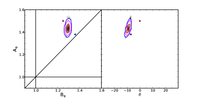
Figure 1: Marginalized PDFs for $A_{\Phi}$, $B_{\Phi}$, and $\theta$ from the MCMC run described in Section 2.4 (TP). Contours enclose 68%, 95%, and 99% of the probability in either the $A_{\Phi}-B_{\Phi}$ or $A_{\Phi}-\theta$ planes (left and right panels, respectively). The black points indicate models from the MCMC run that lie outside the 99% contour. The stars show the best-fit parameters from LMJ09 (red) and LM10 (blue). The diagonal, horizontal, and vertical lines in the left-hand panel are for reference. Models along the diagonal line have $A_{\Phi}=B_{\Phi}$ and are axisymmetric with the symmetry axis coincident with the $x_{t}$ axis. Along the upper portion of this line the models are oblate. Models along the horizontal $A_{\Phi}=1$ line are axisymmetric with the symmetry axis coincident with the $z$-axis (i.e., the symmetry axis of the disk.)

We fit the stream using our SM-MCMC algorithm with 100 walkers and 5000 steps. Here and throughout this work we discard the first 1000 steps, i.e., the burn-in segment of the chain. The marginalized PDFs for $A_{\Phi}$, $B_{\Phi}$, and $\theta$ in this run (referred to as the triaxial potential or TP run) are shown in Figure 1 while a summary is provided in Table 1. Interestingly, the most likely shape from the Bayesian analysis is closer to the results of LM10 than the results from LMJ09. The implication is that the parameter search algorithm is at least as important as whether the Sgr dSph is modeled as an N-body system or a point particle.

	$A_{\Phi}$	$B_{\Phi}$	$A_{\rho}$	$B_{\rho}$	$\theta$
LMJ09	1.5	1.25	(2.5)	(1.75)	$0^{\circ}$
LM10	1.4	1.4	(2.2)	(2.2)	$-7^{\circ}$
TP	1.49	1.34	(2.48)	(2.03)	$-9^{\circ}$
TD	(1.49)	(1.38)	2.48	2.15	$-11^{\circ}$

Table 1: Axis ratios and angle $\theta$ for the LMJ09, LM10 analyses and TP and TD runs as described in Section 2. Parenthesis denote axis ratios that are calculated using the expression $A_{\rho}=3\left(A_{\Phi}-1\right)+1$ or its inverse.

2.5 Triaxial density

By design, isopotential surfaces in the halo model described by Equation 3 are triaxial whereas the isodensity surfaces are not. Indeed, when $A$ and $B$ differ significantly from $1$, as in the best-fit models of LMJ09 and LM10, isodensity surfaces become peanut-shaped (see Fig. 2.9 of Binney & Tremaine (2008)). In simulations, the shape of dark matter halos is inferred by measuring the axis ratios of isodensity surfaces assuming that these are the surfaces that are triaxial. With these issues in mind, we consider an alternative model in which the halo density is given by

$$\rho_{h}(R,z)=\rho_{h}\left(r_{t}^{2}\right)\frac{\sigma_{h}^{2}}{2\pi G}\frac{r^{2}+3d^{2}}{\left(r_{t}^{2}+d^{2}\right)^{2}}$$ (7)

where $\mathbf{r_{t}}\equiv\mathbf{R\Lambda_{\rho}r}$ with $\mathbf{\Lambda_{\rho}}={\rm diag}\left(1,\,A^{-1}_{\rho},\,B^{-1}_{\rho}\right)$. Note that in the spherical limit, $r=r_{t}$ and Equations 7 and 3 describe equivalent models.

The force and potential are calculated from Equation 7 via the homeoid theorem (Binney & Tremaine, 2008). The potential for any triaxial density is given by

$$\Phi(\mathbf{x})=-\pi G\frac{a_{2}a_{3}}{a_{1}}\int_{0}^{\infty}d\tau\frac{\psi(\infty)-\psi(m)}{\sqrt{(\tau+a_{1}^{2})(\tau+a_{2}^{2})(\tau+a_{3}^{2})}}~{},$$ (8)

where the $a_{i}$ are the axis ratios,

$$m^{2}=a_{1}^{2}\sum_{i=1}^{3}\frac{x_{i}^{2}}{a_{i}^{2}+\tau}$$ (9)

is similar to the square of the ellipsoidal radius, and

$$\psi(m)=\int_{0}^{m^{2}}dm^{2}\rho(m^{2})~{},$$ (10)

is an auxiliary function. In our models $a_{1}=1$, $a_{2}=A_{\rho}$, and $a_{3}=B_{\rho}$.

We consider a Galactic model in which Equation 7 rather than Equation 3 describes the halo. We also allow $D_{\rm Sgr}$ to vary within the range of measured values compiled by Kunder & Chaboyer (2009). To be precise, we assume a uniform prior for $D_{\rm Sgr}$ between $22\,{\rm kpc}$ and $28.5\,{\rm kpc}$. Law et al. (2010) found that the effect of varying $D_{\rm Sgr}$ was degenerate with other parameters, particularly the distance $R_{{o}}$ of the Sun to the Galactic center. We therefore include $R_{{o}}$ as a model parameter and assume a Gaussian prior centered on $8.2\,{\rm kpc}$ with 1-$\sigma$ width of $0.4\,{\rm kpc}$ (Bovy, Hogg, & Rix, 2009). We also include a prior probability for the proper motion based on the HST analysis of Pryor et al. (2007). Finally, we replace $\sigma_{\beta,i}$ and $\sigma_{v,i}$ in Equation 5 with the free parameters $\epsilon_{\beta,j}$ and $\epsilon_{v}$, where $j=MG$ for the Majewski et al. (2003) M giants and SDSS for the Belokurov et al. (2006) SDSS fields. That is, we model the stream thickness in both angular position and line-of-sight velocity. To summarize, our model now includes five additional parameters, $D_{\rm Sgr}$, $R_{{o}}$, $\epsilon_{MG}$, $\epsilon_{SDSS}$, and $\epsilon_{v}$.

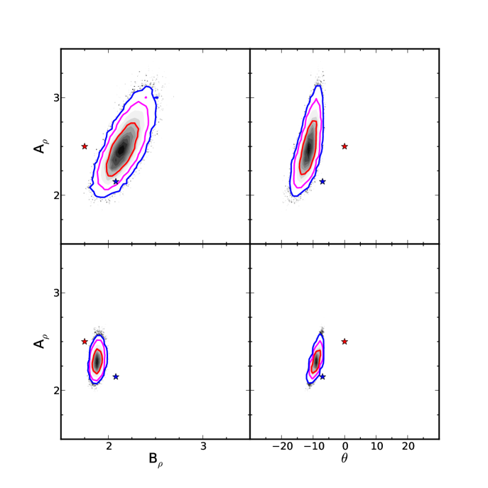
Figure 2: The PDFs for $A_{\rho}$, $B_{\rho}$ and $\theta$ for TD as described in Section 2.5 (upper panels) and TP (lower panels). For the upper panels, $A_{\Phi}$ is transformed to $A_{\rho}$ using the expression $A_{\rho}=3\left(A_{\Phi}-1\right)+1$ and likewise for $B$. The contours, black points, and symbols are the same as in Figure 1.

The marginalized PDFs for $A_{\rho}$, $B_{\rho}$, and $\theta$ are shown in Figure 2 (referred to as the triaxial density or TD run). We also compare the best-fit values with those from the previous analysis and with the results from LMJ09 and LMJ10. To do so, we use the relation $A_{\rho}=3\left(A_{\Phi}-1\right)+1$ from Binney & Tremaine (2008). Once again, we find that the Sgr stream favours a strongly oblate-triaxial halo with isodensity axis ratios that are greater than 2 and with the symmetry axis closely aligned with the Sun-GC line. The uncertainty in the axis ratios is greater, by about a factor of three, for this run.

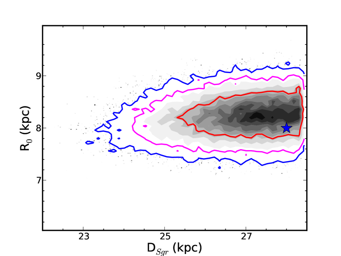
Figure 3: The marginalized PDF in the $R_{{o}}-D_{\rm{Sgr}}$ from TD. The contours and black points are the same as Figure 1. The blue star shows the values assumed by LMJ09 and LM10.

In Figure 3, we show the marginalized PDF in the $D_{\rm Sgr}-R_{{o}}$ plane. The constraint on $R_{{o}}$ comes almost entirely from the prior, while our fit to the stream data favours the upper range of observed values for the distance to the Sgr dSph.

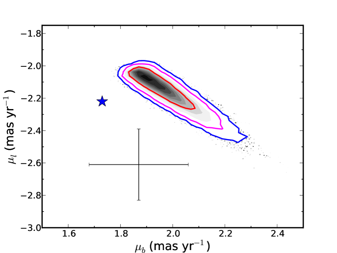
Figure 4: The PDF in the $\mu_{l}-\mu_{b}$ plane. The contours and black points are the same as Fig. 1. The black cross shows the results from the Pryor et al. (2007) analysis. The blue star is the value favoured by LM10.

In Figure 4, we show the marginalized PDF for the components of the proper motion, $\mu_{l}$ and $\mu_{b}$. Evidently, the PDFs are inconsistent with measurements by Pryor et al. (2007) at about the $2\sigma$-level but are consistent with the favoured values obtained in LMJ09 and LM10. Tension between the model and observed values for the proper motion may indicate a problem with the model assumptions (e.g., interpretation of the streams as direct tracers of the orbit) though clearly a more refined measurement of $\mu_{l}$ and $\mu_{b}$ is required.

3 Toward a more realistic Milky Way model

3.1 An updated Galactic model

The model described by Equations 1-3 is attractive in large part because of its simplicity since the potential, force, and density can all be expressed in terms of analytic functions. However, this model does not represent our current understanding of the azimuthally-averaged structure of spiral galaxies. For example, Andredakis, Peletier, & Balcells (1995) showed that bulges of spiral galaxies could be best fit by the Sérsic law. Furthermore, since the classic paper by Freeman (1970), it has become standard practice to model the luminosity profile of disks as an exponential. Finally, the spherically-averaged density profile of dark matter halos is described extremely well by the Einasto profile (Merritt et al., 2006). Therefor we consider a Milky Way model with these three components. We assume that the bulge and disk have constant (but different) mass-to-light ratios. The density that produces a Sérsic surface brightness profile is (Prugniel & Simien, 1997; Terzić & Graham, 2005)

$$\rho_{b}(r)=\rho_{b0}\left(\frac{r}{R_{e}}\right)^{-p}e^{-b(r/Re)^{1/n}}~{},$$ (11)

where $p=1-0.6097/n+0.05563/n^{2}$, $n$ is the Sérsic index and $b=b(n)$ is chosen so that the radius $R_{e}$ encloses half the total projected mass. For simplicity, we parameterize the bulge by the scale velocity

$$\sigma_{b}\equiv\left(4\pi nb^{n\left(p-2\right)}\Gamma\left(n\left(2-p\right)\right)R_{e}^{2}\rho_{b0}\right)^{1/2}$$ (12)

rather than $\rho_{b0}$.

We assume that the disk density is exponential in the radial direction (the Freeman Law) and has a sech² structure in the vertical direction:

$$\rho_{d}\left(R,\,z\right)=~{}\frac{M_{d}}{4\pi R_{d}^{2}z_{d}}\,e^{-R/R_{d}}\,{\rm sech}^{2}\left(z/z_{d}\right)$$ (13)

where $M_{d}$, $R_{d}$, and $z_{d}$ are the mass, radial scale length, and vertical scale height for the disk, respectively. The disk potential is calculated using the technique of Kuijken & Dubinski (1995). An analytic ’fake’ disk density-potential pair, $\left(\rho_{fd},\,\Phi_{fd}\right)$ is constructed so that $\rho_{d}=\rho_{fd}+\rho_{r}$ and $\Phi_{d}=\Phi_{fd}+\Phi_{r}$ where $\left(\rho_{r},\,\Phi_{r}\right)$ is the density-potential pair of the residual. The fake disk is designed to account for the high-order moments of the disk potential. The full potential is calculated by solving the Poisson equation using a spherical harmonics expansion and iterative scheme.

The density distribution for our halo model is given by

$$\rho_{h}(r_{t})=\rho_{0}e^{-\frac{2}{\alpha}((r_{t}/r_{h})^{\alpha}-1)}$$ (14)

where $r_{t}$ is the triaxial radius, $\rho_{0}$ is a scale density, $r_{h}$ is the scale radius, and $\alpha$ controls the logarithmic slope of the density profile. The potential for this triaxial density is calculated via Equation 8.

To be sure this model represents an approximation to the mass distribution and gravitational potential of the Galaxy. The model disk and bulge are axisymmetric whereas the actual bulge is triaxial and the disk contains a bar. It is reasonable to ask whether these non-axisymmetric structures could mimic the effects of a triaxial halo. We note that at pericenter the Sgr dSph is $\sim 20$ kpc from the Galactic center whereas the bulge triaxiality and the bar are properties of the inner few kpc. At pericenter, the disk and bulge contribute $\sim 25\%$ and $10\%$ respectively to the gravitational force. Furthermore, the components of the potential associated with the bar and bulge triaxiality are quadruple (or higher order) terms, which fall off significantly faster than the leading monopole term. We therefore conclude that the triaxiality of the bulge and the presence of a bar will have little effect on the orbit of the Sgr dSph and its stream.

3.2 Observational constraints

Our analysis combines kinematic and photometric observations that constrain the structure of the Milky Way across five orders of magnitude in radius. Apart from the constraints due to the Sgr stream, the observations we consider are similar to those found in (Dehnen & Binney, 1998; Widrow & Dubinski, 2005; Widrow, Pym, & Dubinski, 2008) with some notable exceptions. The starting point is a generalization of Equation 5 to

$$p(D|\mathbf{\Theta})=\prod_{i=1}^{N_{\rm{obs}}}\prod_{j}^{N_{i}}\frac{1}{2\pi\sigma_{i,j}}e^{\frac{(M_{i,j}-O_{i,j})^{2}}{2\sigma_{i,j}^{2}}}~{},$$ (15)

where the index $i$ runs over the different types of observational constraints (e.g. stream angular position and radial velocity) while the index $j$ runs over individual data points of a particular type of observation. The model prediction is $M$, the observation, $O$, and is the associated error, $\sigma$.

The stream constraints are as before with one proviso: Since we are treating the Sun’s motion relative to the Galactic centre as a free parameter, we cannot use the GSR radial velocities for the M giants as published in Majewski et al. (2003) but must use the (observed) heliocentric velocities and convert to the GSR using the model values for $v_{c}(R_{{o}})$, $U_{\odot}$, $V_{\odot}$, and $W_{\odot}$.

For the innermost region of the Galaxy, we use the compilation of bulge LOSVD measurements found in Tremaine et al. (2002), with the restriction that $r\geq 4~{}\rm{pc}$ to avoid complications from the central black hole. In addition, we adjust the dispersion downwards by a factor of 1.07 to account for the non-spherical nature of the bulge. We also use the surface brightness profile at infrared wavelengths from the COBE-DIRBE observations (Binney, Gerhard, & Spergel, 1997). These observations extend from $-40^{\circ}$ to $40^{\circ}$ in Galactic longitude and allow us to probe the structure of both the bulge and disk. Of course, our model must now include mass-to-light ratios for the bulge and disk.

We include a number of “local” or solar neighborhood constraints in our analysis. Recently Reid et al. (2009) used Very Long Baseline radio observations to determine trigonometric parallaxes and proper motions for masers throughout the Milky Way’s disk. These measurements were then used to infer a circular speed at the position of the Sun of $254\pm 16\,{\rm km~{}s^{-1}}$, a value 15% higher than the one assumed in LMJ09 and LM10. The Reid et al. (2009) results were scrutinized by Bovy et al. (2009) who carried out a Bayesian analysis of the maser data and also incorporated proper motion measurements of Sgr A^∗. For our analysis, we adopt the Bovy et al. (2009) value: $v_{c}\left(R_{{o}}\right)=244\pm\,13\,{\rm km~{}s^{-1}}$.

The shape of the circular speed curve in the solar neighborhood is described by the Oort constants. We adopt the constraints $A=14.8\pm 0.8~{}{\rm km~{}s^{-1}}\textrm{kpc}^{-1}$ and $B=-12.4\pm 0.6~{}{\rm km~{}s^{-1}}\textrm{kpc}^{-1}$ from Feast & Whitelock (1997). We use the disk surface density measurement of $\Sigma_{d}=49\pm 9~{}{\rm~{}M_{\odot}}~{}\rm{pc}^{-3}$ from Flynn & Fuchs (1994) and the vertical force measurement of $|K_{z}(1.1~{}\textrm{kpc})|=\left({2\pi G}\right)71\pm 6~{}{\rm~{}M_{\odot}}\textrm{pc}^{-2}~{},$ from Kuijken & Gilmore (1991). These values are in good agreement with similar studies (see, for example, Holmberg & Flynn (2004)).

Observations of the Galactic circular speed curve are typically divided into measurements inside and outside the solar circle. The inner rotation curve is usually presented in terms of the terminal velocity, which is defined as the peak velocity along a particular line-of-sight defined by the Galactic coordinates $b=0$ and $l$ where $|l|<\pi/2$. If we assume that the Galaxy is axisymmetric, then $v_{\rm term}=v_{c}\left(R\right)-v_{c}\left(R_{{o}}\right)\sin{l}$. We use data from Malhotra (1995) with the restriction that $\sin l\geq 0.3$ so as to avoid distortions due to the bar. The outer rotation curve requires a more in depth discussion. The circular speed $v_{c}(R)$ is related to the observed line-of-sight velocity $v_{lsr}$ of a kinematic tracer in the disk through the expression

$$W(R)=\frac{R_{{o}}}{R}\,v_{c}(R)-v_{c}(R_{{o}})=\frac{v_{lsr}}{\cos b\cos l}~{}.$$ (16)

We use observations of HII regions and reflection nebulae from Brand & Blitz (1993) and Carbon stars from Demers & Battinelli (2007) with the restriction that $l\leq 155^{\circ}$ or $l\geq 205^{\circ}$, $d\geq 1$ kpc, and $W\leq 0$ so as to avoid complications due to non-circular motions. The errors in the measurements are propagated to errors in $W$. Additionally, ’noise’ parameters for $d$ and $v_{lsr}$ are added in quadrature to the quoted errors to account for the potential for unknown systematic errors. That is, the velocity error for the $j$’th data point is $\sigma_{v}^{2}=\sigma^{2}_{v,m}+\epsilon^{2}_{u}$ where $\sigma_{v,m}$ is the measured error (the $i$ subscript has been suppressed) and $\epsilon_{u}$ is the noise parameter. Similarly, we have $\sigma_{d}^{2}=\sigma^{2}_{d,m}+d^{2}\epsilon^{2}_{d}$. Note that we allow for different noise parameters for the Brand & Blitz (1993) and Demers & Battinelli (2007) data sets.

Finally, we follow Dehnen & Binney (1998) and use $M(r<100\textrm{ kpc})=(7\pm 2.5)\times 10^{11}{\rm~{}M_{\odot}}$ as a constraint on the mass of the Milky Way at large Galactocentric radii. This constraint is based on the study of satellite kinematics by Kochanek (1996), the locally determined ’escape’ speed, and the timing of the local group. It is also based on modelling of the Magellanic Clouds and stream by Lin, Jones, & Klemola (1995). The large error in $M\left(r<100\,{\rm kpc}\right)$ reflects the potential for large systematic errors. In principle, the Sgr system should be able to constrain the mass distribution of the Milky Way in the $30-100\,{\rm kpc}$ range.

4 Results

We now present results based on the constraints described in the preceding Section. As before we use the SM-MCMC algorithm with 100 walkers and 5000 steps. Our model is described by twenty-eight free parameters: nine structural parameters for the disk, bulge and halo, mass-to-light ratios for the bulge and disk, two axis ratios and an orientation angle for the triaxial halo, the distance of the Sun to the Galactic center and its motion relative to the local standard of rest, the heliocentric distance to the Sgr dSph and its proper motion, and seven “noise” parameters. The initial angular position and heliocentric velocity of the Sgr dSph are held fixed. Our priors for the disk scale length and scale height are based on Jurić et al. (2008) while our priors for the Sun’s peculiar velocity are based on values from Binney & Merrifield (1998).

In Table 2 we present a summary of the statistics for the model parameters. In particular, we give the mean and variance of the marginalized PDF for each parameter. For convenience, we also list the prior used for each parameter.

$\Theta$	$\langle\Theta\rangle$	${\rm Var}\left(\Theta\right)^{1/2}$	Prior	Lower Limit	Upper Limit
$n$	1.77	0.37	uniform	0.6	4.
$\sigma_{b}$	314	23	log	100.	500.
$r_{e,b}$	0.60	0.07	log	0.1	2.
$M/L_{b}$	0.69	0.20	uniform	0.4	2.
$M/L_{d}$	1.09	0.08	uniform	0.4	2.
$M_{d}$	$5.2\times 10^{10}$	$0.5\times 10^{10}$	log	$1.8\times 10^{10}$	$7.0\times 10^{11}$
$\rho_{0}$	$1.4\times 10^{-3}$	$0.4\times 10^{-3}$	log	$2\times 10^{-3}$	$7\times 10^{-3}$
$r_{e,h}$	11.1	1.3	log	2	35
$\alpha$	0.23	0.07	uniform	0	0.5
$A$	3.58	0.45	log	1	5
$B$	2.58	0.25	log	0.2	5
$\theta$	-5.4∘	$1.4^{\circ}$	uniform	$-90^{\circ}$	$90^{\circ}$
$d$	25.	1.	uniform	22	28.5
$\epsilon_{d,B}$	0.42	0.05	log	0.01	0.7
$\epsilon_{v,B}$	3.7	1.4	log	1	60
$\epsilon_{d,D}$	0.49	0.03	log	0.01	0.7
$\epsilon_{v,D}$	53.	14.	log	1	60
$\epsilon_{\rm MG}$	6.9	0.5	uniform	1	20
$\epsilon_{\rm SDSS}$	3.0	1.3	uniform	1	20
$\epsilon_{u}$	33.	18.	uniform	1	40
			Prior	Width	Mean
$R_{e.d}$	2.80	0.12	Gaussian	1.	3.5
$Z_{e,d}$	0.48	0.08	Gaussian	0.06	0.3
$U_{\odot}$	-9.8	0.04	Gaussian	0.4	-10.0
$V_{\odot}$	-5.6	0.7	Gaussian	0.6	-5.25
$W_{\odot}$	7.3	0.4	Gaussian	0.4	7.2
$R_{{o}}$	8.4	0.2	Gaussian	0.4	8.2
$\mu_{l}$	-2.39	0.16	Gaussian	0.22	-2.61
$\mu_{b}$	1.91	0.13	Gaussian	0.19	1.87

Table 2: Statistical summary of results from the MCMC run described in Section 4. Column 1 — parameter; column 2 — mean value; column 3 — variance; column 4 — type of prior used. Columns 5 and 6 give the lower and upper bounds for prior in the case of either a uniform or log prior and the width and mean for the case where the prior is a Gaussian. The units are ${\rm km~{}s^{-1}}$, kpc, ${\rm~{}M_{\odot}}$, ${\rm~{}M_{\odot}}~{}\textrm{pc}^{-3}$, $\textrm{mas yr}^{-1}$ for velocity, distance, mass, density, and proper motions respectively.

4.1 General properties of the Galaxy

Table 3 presents a summary of the statistics for the observables based on our MCMC analysis. For comparison, we include the predictions from the LJM model. We see that our analysis favors a somewhat lower value for the circular speed than advocated by Bovy et al. (2009) though the discrepancy is only at the $1.5\sigma$-level. More importantly, our model is consistent with estimates for both the disk surface density and vertical force in the solar neighborhood in contrast with the LJM model, which predicts values that are too high, implying that their disk mass is too large.

Observation	Observed	LJM	This Work
$v_{c}$ (${\rm km~{}s^{-1}}$)	$244\pm 13$	$220$	$225\pm 4$
Oort $A$ (${\rm~{}km~{}s^{-1}~{}kpc^{-1}}$)	$14\pm 0.8$	$13.0$	$14.4\pm 0.3$
Oort $B$ (${\rm~{}km~{}s^{-1}~{}kpc^{-1}}$)	$-12.4\pm 0.6$	$-14.5$	$-12.6\pm 0.4$
$\Sigma_{d}$ (${\rm~{}M_{\odot}}\textrm{pc}^{-2}$)	$49\pm 9$	$95$	$49\pm 4$
$\left(2\pi G\right)^{-1}{|K_{z}(1.1~{}\textrm{kpc})|}$ (${\rm~{}M_{\odot}}\textrm{pc}^{-2}$)	$71\pm 6$	$100.1$	$75\pm 5$
$M(r<100~{}\textrm{kpc})$ ($10^{11}{\rm~{}M_{\odot}}$)	$7\pm 2.5$	$7.96$	$6.99\pm 0.63$

Table 3: Mean values for observables from the LJM model and this work.

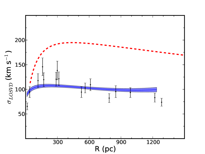
Figure 5: Velocity dispersion profile as a function of projected radius. The thin blue line shows the velocity dispersion averaged over the chain. The shaded region gives the 68% credible region. The red dashed curve is the prediction for the LJM model. The black points are from Tremaine et al. (2002).

In Figure 5 we show the LOSVD measurements from Tremaine et al. (2002) and the inferred values from the model. Our model does a good job in matching the general value for the dispersion profile though the data show a clear peak at 200 pc and decline for larger radii whereas the model dispersion profile is relatively flat. The implication is that the simple Sérsic-Prugniel & Simion model may be inadequate for the inner-most regions of the bulge. We see that the LJM model predicts LOSVD’s that are 1.5-2 times higher than the measured velocities, which implies that their bulge mass is 2-4 times to high.

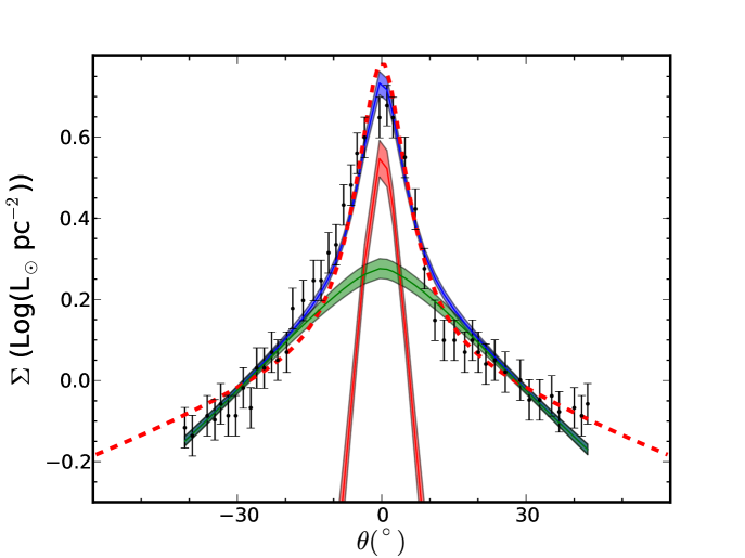
Figure 6: Surface brightness as a function $l$. The thin lines and shaded regions are the average and 68% credible regions for the total surface brightness (blue), the bulge (red) and the disk (green). The dashed red curve is prediction for the LJM model.

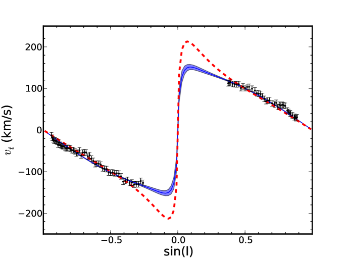
Figure 7: Terminal velocity as a function of $\sin{l}$. The thin blue line and shaded region are the average and 68% credible region, respectively while the dashed red curve shows the prediction for the LMJ model. The black points are the data from Malhotra (1995).

The surface brightness toward the bulge is shown in Figure 6. Both our model and the LJM model do an acceptable job in fitting the data. The inner rotation curve is shown in Figure 7 and again, an acceptable fit is obtained. Note that the LJM prediction rises more steeply at small $|l|$ as compared with our model and reaches a peak circular speed that is higher by a factor of 1.5.

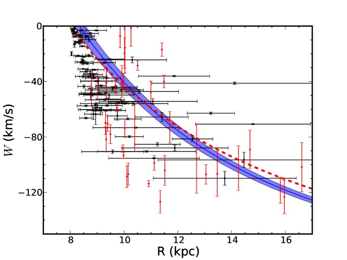
Figure 8: Outer rotation curve as a function of projected radius $R$. The curves are as in Figure 5. The black points are from Brand & Blitz (1993) and the red points are from Demers & Battinelli (2007).

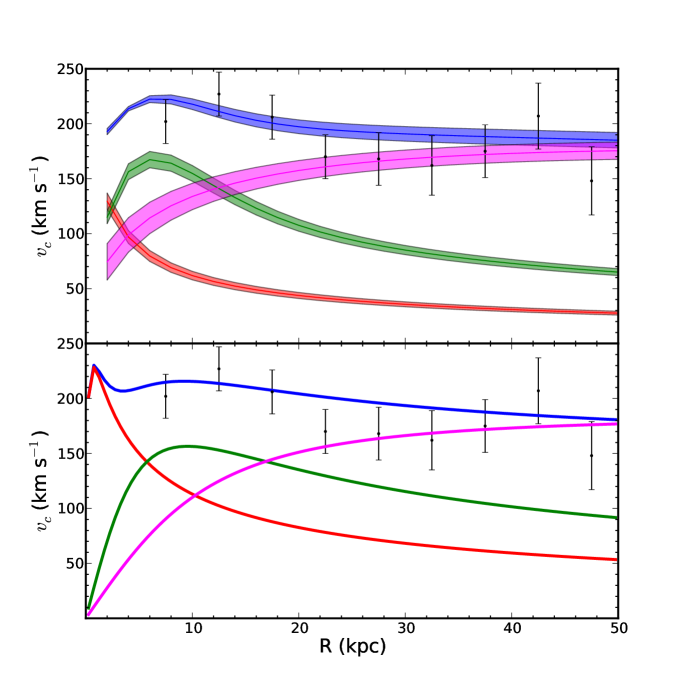
Figure 9: Composite curcular speed curve as a function of radius. Lines and shaded regions show the average the 68% credible regions (upper panel) for the total circular speed curve (blue) and the contributions from the bulge (red), disk (green), and halo (magenta). The dashed curves (lower panel) are the prediction from the LJM model. Black points are from Xue et al. (2008). These points are not used in the fit but are shown as a consistency check.

We show the outer rotation curve in Figure 8. In contrast with the inner regions of the Galaxy, the LJM model and ours have a very similar shape. This point is further illustrated in Figure 9 where we show the full circular speed curve across a wide range in radii. For comparison, we also show the Xue et al. (2008) rotation curve, though this data was not used in our analysis. The LJM model and ours yield remarkably similar circular speed curves even though the bulge-disk-halo decomposition of $v_{c}$ is very different. We note that the peak contribution to $v_{c}$ from the bulge is nearly twice that for our best-fit model, a result echoed in Figure 5 The peak contribution to $v_{c}$ from the disk is roughly the same in the LJM model as in our best-fit model, though in the LJM model, the peak occurs at R=10 kpc whereas in ours, it occurs at about 5-6 kpc. Recall that for an exponential disk, the peak in $v_{c}$ is at 2.2 disk scale lengths, so the implication is that the LJM disk has an effective scale length of   5 kpc, which is roughly a factor of two larger than the standard values for the Milky Way.

4.2 The Sgr stream and halo triaxiality

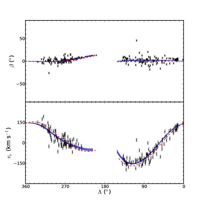
Figure 10: Angular postion and line-of-sight velocity as a function of position along the stream. The upper panel shows the angular position perpendicular to the stream, $\beta$, as a function of angular position along the stream, $\lambda$. The lower panel shows the heliocentric radial velocity, $v_{r}$, as a function of $\lambda$. The thin blue line, shaded region, and dashed curve are as in Figure 5. The black points are the 2MASS M giants while the red stars are the Belokurov et al. (2006) SDSS fields. The red dashed line is the predictions for the best-fit model of LMJ09. While the LM10 should be considered superior to the LMJ09 model, it produces the fit to the data using an N-body representation of the dwarf rather than the single particle approximation. Since we also use the single particle approximation, it is more appropriate to show that comparison.

In Figure 10 we show the angular position $\beta$ and heliocentric velocity $v_{r}$ of stars that are presumed to be members of the Sgr stream. A few comments are in order. First, the M-giant data is considerably noisier than the SDSS fields though the latter only covers a portion of the leading arm of the Sgr stream. In Table 2, the stream-thickness (or noise) parameters are $\epsilon_{\rm MG}=6.9^{\circ}$ and $\epsilon_{\rm SDSS}=3^{\circ}$. Thus, the analysis accounts for the intrinsic scatter in the M-giant data by choosing a larger noise parameter. This choice has the effect of reducing the weight the individual M-giant data points as compared with the SDSS fields in the likelihood calculation.

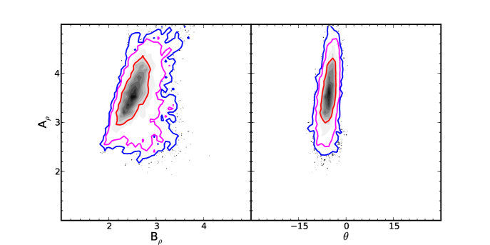
Figure 11: Marginalized PDFs for $A_{\rho}$, $B_{\rho}$, and $\theta$ for the model introduced in Section 4. Contours, points and symbols are the same as those used in Figure 1.

The PDFs for $A_{\rho}$, $B_{\rho}$, and $\theta$ are shown in Figure 11. The inferred shape is still roughly oblate with the short axis nearly aligned with the Sun-GC line. In fact, the preferred model is more strongly aspherical; the best-fit values for $A_{\rho}$ and $B_{\rho}$ are even larger than were found in the analysis presented in Section 2. Note however that the uncertainties in these values is larger than before.

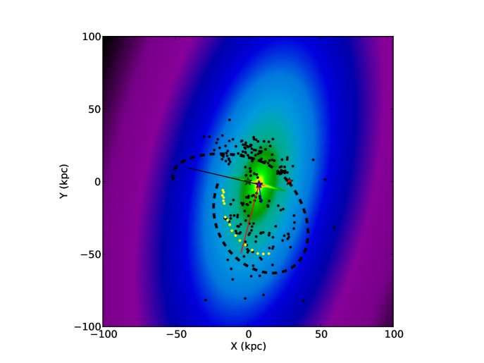
Figure 12: Total Milky Way density and the Sgr stream in the $\beta=0$ plane. The green, blue, and red stars show the location of the Sun, GC, and Sgr dwarf respectively. The black points show the Sgr stream M Giants and the yellow points show the SDSS fields from Belokurov et al. (2006). The dashed curve shows the orbit of the dwarf in the Milky Way model with the parameters equal to the expectation values from Table 2. The solid blue, red, and black lines show the $A$, $B$, and $1$ axes respectively.

Regardless of the model or the suite of constraints, the Sagittarius stream consistently points to a halo model that is oblate-triaxial with the short axis of the halo approximately coincident with the Sun-GC line. What properties of the Sgr stream drive the fit of the halo in this direction? In Figure 12 we show the isodensity contours for the total Milky Way model in the $\beta=0$ plane. Also shown are the principle axes of the halo projected on to this plane. Finally, we show positions of the M giant and SDSS fields along the stream. Roughly speaking, the stream (and presumably, the orbit of the Sgr dSph) are elongated parallel to the plane of the disk. In general, if isopotential surfaces in a particular plane are ellipses, then at least some of the particle orbits in that plane will be elongated perpendicular to the long axis of the potential. Thus, current observations of the Sgr stream may require a halo that is elongated perpendicular to the plane of the Galactic disk, as found in LMJ09, LM10 and in the present work.

4.3 Mass distribution

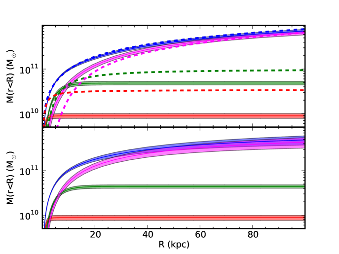
Figure 13: Cumulative mass profile as a function of spherical radius $r$. Solid lines and shaded regions show the average values 68% credible region for the total (blue) and the separate contribution of the bulge (red), disk (green), and halo (magenta). The dashed red line shows the predictions of the LJM model. The upper panel shows $M(r)$ with the full suite of constraints, include the data for the Sgr Stream. The lower panel shows $M(r)$ when the stream data is not used.

The Sgr stream inhabits the region of the Galaxy between 20-60 kpc, which is roughly where the gravitational potential transitions from disk-dominated to halo-dominated. The stream therefore has the potential to help break the disk-halo degeneracy and constrain the mass distribution beyond the disk. To explore this point, we re-analyze the model without the Sgr stream constraint. The result for the cumulative mass profile is shown in Figure 13. We see that uncertainties in the mass at $r=100$ kpc are reduced from 0.3 dex to 0.1 dex by including the Sgr stream,.

As noted above, and illustrated in Figure 13, the mass distribution for our model and for the LJM model are very similar though the mass decomposition are very different. In particular, the disk and bulge masses for our model are lower in our models by factor of 2-4.

5 Conclusions

We have performed a Bayesian analysis designed to model Milky Way that incorporates data for the Sgr stream together with a broader suite of observational constraints. Our analysis allows us to not only infer the shape of the dark matter halo, but also its spherically-averaged mass distribution. We find that our Bayesian approach, which uses single-particle orbits, yields results for the shape parameters of the halo that are consistent with the N-body-based approach of LM10. Moreover, the Sgr stream reduces the uncertainty in the Milky Way mass profile by a factor of $\sim 2$.

Our analysis has not resolved the central question posed by LMJ09 and LM10: Why does the Sgr stream appear to favour such a strongly triaxial halo? As discussed in the introduction, triaxial halo models favoured by LMJ09, LM10, and this work are outliers in the distribution of halo shapes predicted by the standard $\Lambda$-CDM cosmology. While the Galactic halo may indeed have this shape, we caution the reader that these analyses make use of a single stream. One should be suspicious that the halo model shares the same approximate orientation as the orbital plane of the Sgr stream.

In principle, the use of multiple stellar streams with different orbital planes can improve the situation. Indeed, the GD-1, Orphan, and Monoceros streams have been already been extensively studied and, in some cases, used to constrain Milky Way models (see, for example Koposov, Rix, & Hogg (2010); Newberg et al. (2010); Peñarrubia et al. (2005)). As discussed in Koposov, Rix, & Hogg (2010), the GD-1 stream is a particular attractive feature since it is extremely narrow and therefore has a simple internal structure as compared with the Sgr stream. However, the GD-1 and Orphan streams cover a significantly smaller angular extent than the Sgr stream and therefore may have limited value in constraining the potential.

The tidal debris of satellite galaxies may, in fact, provide other less direct clues about halo triaxiality. N-body simulations by Rojas-Niño et al. (2012) (see also Peñarrubia, Walker, & Gilmore (2009)) suggest that the morphology of tidal debris depends on the shape of the host galaxy’s halo and in particular, the degree to which it departs from spherical symmetry.

The results presented in this work and in LMJ09 and LM10 provide a tantilizing, if not unsettling picture of the Galactic halo. Clearly, further analysis and more data are required to establish what the shape of the dark halo is. Advances will likely come from a combination of improved modelling techniques, detailed N-body simulations and new data from the the next generation of surveys, such as Gaia Perryman (2002) and LSST Ivezic et al. (2008).

We thank K. Johnston, R. Ibata, D. Hogg, and D. Foreman-Mackey for insightful comments and suggestions. LMW acknowledges the financial support of the Natural Sciences and Engineering Research Council of Canada through the Discovery Grant program. This research made use of the Python programming language and the open-source modules numpy and matplotlib.

References

- Allgood et al. (2006) Allgood B., Flores R. A., Primack J. R., Kravtsov A. V., Wechsler R. H., Faltenbacher A., Bullock J. S., 2006, MNRAS, 367, 1781
- Andredakis, Peletier, & Balcells (1995) Andredakis Y. C., Peletier R. F., Balcells M., 1995, MNRAS, 275, 874
- Belokurov et al. (2006) Belokurov V. et al., 2006, ApJ, 642, L137
- Binney et al. (1997) Binney J., Gerhard O., Spergel D., 1997, MNRAS, 288, 365
- Binney & Merrifield (1998) Binney J., Merrifield M., 1998, Galactic Astronomy. Princeton Univ. Press, Princton, NJ
- Binney & Tremaine (2008) Binney J., Tremaine S., 2008, Galactic Dynamics: Second Edition. Princeton Univ. Press, Princton, NJ
- Bovy et al. (2009) Bovy J., Hogg D. W., Rix H.-W., 2009, ApJ, 704, 1704
- Brand & Blitz (1993) Brand J., Blitz L., 1993, A&A, 275, 67
- Debattista et al. (2008) Debattista V. P., Moore B., Quinn T., Kazantzidis S., Maas R., Mayer L., Read J., Stadel J., 2008, ApJ, 681, 1076
- Dehnen & Binney (1998) Dehnen W., Binney J., 1998, MNRAS, 294, 429
- Demers & Battinelli (2007) Demers S., Battinelli P., 2007, A&A, 473, 143
- Dubinski (1994) Dubinski J., 1994, ApJ, 431, 617
- Feast & Whitelock (1997) Feast M., Whitelock P., 1997, MNRAS, 291, 683
- Fellhauer et al. (2006) Fellhauer M. et al., 2006, ApJ, 651, 167
- Flynn & Fuchs (1994) Flynn C., Fuchs B., 1994, MNRAS, 270, 471
- Foreman-Mackey et al. (2012) Foreman-Mackey D., Hogg D. W., Lang D., Goodman J., 2012, arXiv:1202.3665 [astro-ph.IM]
- Franx et al. (1991) Franx M., Illingworth G., de Zeeuw T., 1991, ApJ, 383, 112
- Freeman (1970) Freeman K. C., 1970, ApJ, 160, 811
- Frenk (1988) Frenk C. S., 1988, in Audouze J., Pelletan M.-C., & Szalay S., eds Proc. IAU Symp., 130, Large Scale Structures of the Universe, p. 259
- Goodman & Weare (2010) Goodman J., Weare J., 2010, Comm. App. Math. Comp. Sci., 65, 5
- Helmi (2004) Helmi A., 2004, ApJ, 610, L97
- Hernquist (1990) Hernquist L., 1990, ApJ, 356, 359
- Holmberg & Flynn (2004) Holmberg J., Flynn C., 2004, MNRAS, 352, 440
- Ibata et al. (2001) Ibata R., Lewis G. F., Irwin M., Totten E., Quinn T., 2001, ApJ, 551, 294
- Ibata et al. (1997) Ibata R. A., Wyse R. F. G., Gilmore G., Irwin M. J., Suntzeff N. B., 1997, AJ, 113, 634
- Ivezic et al. (2008) Ivezic, Z. et al. 2008, arXiv:0805.2366v2 [astro-ph]
- Jing & Suto (2002) Jing Y. P., Suto Y., 2002, ApJ, 574, 538
- Johnston et al. (2005) Johnston K. V., Law D. R., Majewski S. R., 2005, ApJ, 619, 800
- Johnston et al. (1999) Johnston K. V., Majewski S. R., Siegel M. H., Reid I. N., Kunkel W. E., 1999, AJ, 118, 1719
- Jurić et al. (2008) Jurić M. et al., 2008, ApJ, 673, 864
- Kazantzidis et al. (2004) Kazantzidis S., Kravtsov A. V., Zentner A. R., Allgood B., Nagai D., Moore B., 2004, ApJ, 611, L73
- Kochanek (1996) Kochanek C. S., 1996, ApJ, 457, 228
- Koposov, Rix, & Hogg (2010) Koposov, S. E., Rix, H.-W., Hogg, D. W., 2010, ApJ, 712, 260
- Kuijken & Dubinski (1995) Kuijken K., Dubinski J., 1995, MNRAS, 277, 1341
- Kuijken & Gilmore (1991) Kuijken K., Gilmore G., 1991, ApJ, 367, L9
- Kunder & Chaboyer (2009) Kunder A., Chaboyer B., 2009, AJ, 137, 4478
- Law et al. (2010) Law D. R., Johnston K. V., Majewski S. R., 2005, ApJ, 619, 807
- Law & Majewski (2010) Law D. R., Majewski S. R., 2010, ApJ, 714, 229
- Law et al. (2009) Law D. R., Majewski S. R., Johnston K. V., 2009, ApJ, 703, L67
- Lin, Jones, & Klemola (1995) Lin D. N. C., Jones B. F., Klemola A. R., 1995, ApJ, 439, 652
- Majewski et al. (2003) Majewski S. R., Skrutskie M. F., Weinberg M. D., Ostheimer J. C., 2003, ApJ, 599, 1082
- Majewski et al. (2004) Majewski S. R. et al. 2004, AJ, 128 245
- Malhotra (1995) Malhotra, S., 1995, ApJ, 448, 138
- Martínez-Delgado et al. (2004) Martínez-Delgado D., Gómez-Flechoso M. Á., Aparicio, A., Carrera R., 2004, ApJ, 601, 242
- Merritt et al. (2006) Merritt D., Graham A. W., Moore B., Diemand J., Terzić B., 2006, AJ, 132, 2685
- Miyamoto & Nagai (1975) Miyamoto M., Nagai R., 1975, PASJ, 27, 533
- Newberg et al. (2010) Newberg, H. J., Willett, B. A., Yanny, B., Xu, Y., 2010, ApJ, 711, 32
- Peñarrubia, Walker, & Gilmore (2009) Peñarrubia, J., Walker, M. G., Gilmore, G. 2009, MNRAS, 399, 1275
- Peñarrubia et al. (2005) Peñarrubia, J. et al., 2005, ApJ, 626, 128
- Perryman (2002) Perryman, M. A. C., 2002, AP&SS, 280, 1
- Prugniel & Simien (1997) Prugniel P., Simien F., 1997, A&A, 321, 111
- Pryor et al. (2007) Pryor, C., Piatek S., Olszewski E. W., 2010, AJ, 139, 839
- Reid et al. (2009) Reid M. J. et al., 2009, ApJ, 700, 137
- Rojas-Niño et al. (2012) Rojas-Niño, A., Valenzuela, O., Pichardo, B., & Aguilar, L. A. 2012, 757, L28
- Terzić & Graham (2005) Terzić B., Graham A. W., 2005, MNRAS, 362, 197
- Tremaine et al. (2002) Tremaine S. et al. 2002, ApJ, 574, 740
- Varghese et al. (2011) Varghese, A. Ibata, R. Lewis, G. F., 2011, MNRAS, 417, 198
- Warren et al. (1992) Warren M. S., Quinn P. J., Salmon J. K., Zurek W. H., 1992, ApJ, 399, 405
- Widrow & Dubinski (2005) Widrow L. M., Dubinski J., 2005, ApJ, 631, 838
- Widrow et al. (2008) Widrow L. M., Pym B., Dubinski J., 2008, ApJ, 679, 1239
- Xue et al. (2008) Xue X. X. et al., 2008, ApJ, 684, 1143