Lattice models in biological physics Filaments in subcellular structure and processes Flagella

Modelling bacterial flagellar growth

Abstract

The growth of bacterial flagellar filaments is a self-assembly process where flagellin molecules are transported through the narrow core of the flagellum and are added at the distal end. To model this situation, we generalize a growth process based on the TASEP model by allowing particles to move both forward and backward on the lattice. The bias in the forward and backward jump rates determines the lattice tip speed, which we analyze and also compare to simulations. For positive bias, the system is in a non-equilibrium steady state and exhibits boundary-induced phase transitions. The tip speed is constant. In the no-bias case we find that the length of the lattice grows as $N(t)\propto\sqrt{t}$, whereas for negative drift $N(t)\propto\ln{t}$. The latter result agrees with experimental data of bacterial flagellar growth.

Bacterial flagella act as motility devices that allow bacteria such as Escherichia coli and Salmonella to swim and to respond to chemical stimuli by performing chemotaxis [1]. A flagellum mainly consists of a long helical hollow structure with a length of up to $20\mu m$ and a typical outer diameter of $0.02\mu m$. The growth mechanism of the flagellar filament is a self-assembly process. Flagellin molecules are transported through the hollow core of the filament and are added one by one at the tip of the filament. An important quantity of such a growth process is the time dependence of the filament length $N(t)$. A recent model that treats flagellin molecules as diffusing particles in a single-file process established a growth function $N(t)\propto\sqrt{t}$ [2]. However, the only available experimental data to our knowledge show a logarithmic growth $N(t)\propto\ln t$ [3]. To model the growth process and to try to verify the experimental data, we make use of a variant of the well known totally asymmetric simple exclusion process (TASEP). This model takes into account the important fact that flagellar growth happens in a single-file process meaning flagellin molecules cannot pass each other.

The TASEP itself has developed into a paradigmatic model of non-equilibrium physics [4, 5, 6, 7, 8, 9]. In particular, TASEP models with open boundaries showed to be very fruitful for the study of non-equilibrium steady states, i.e., states that are characterized by non-vanishing currents. These systems have been used to model the motion of ribosome along mRNA [10], molecular motors along microtubule filaments [11], or that of cars on a highway [12, 13], just to name a few applications. All of these models consider lattices with a fixed number of lattice sites $N$. However, there are recent approaches that generalize the TASEP to dynamically extending exclusion processes. One approach considers the TASEP with a fluctuating boundary that can be pushed away by particles on the lattice [14], another one takes into account a death probability of the leading particle [15, 16]. In a different variant of the TASEP, particles that reach the end of the lattice can transform into new lattice sites resulting in a dynamically extending lattice [17]. Initially, the extending TASEP was formulated to model fungal hyphal growth [18]. In the reminder of this paper we will generalize this model to a partially asymmetric model where particles can move both forward and backward on the lattice. In particular, we calculate the growth function $N(t)$ and discuss implications for the bacterial flagellar growth.

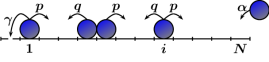
Figure 1: Growing asymmetric simple exclusion process with open boundary conditions. The labels indicate rates at which particle hops can occur. At site $1$ particles transform into a new lattice site with rate $\gamma$, which then becomes the new site 1.

The model is defined in the following way (see fig. 1 for a schematic). Particles enter the lattice with rate $\alpha$ at the boundary on the right. They either move to the left with rate $q$ or to the right with rate $p$ so that $q+p=1$. Finally, at the tip of the lattice at site $1$ they transform into a new lattice site with rate $\gamma$. A crucial feature of TASEP models is that particles can only move if the target site is empty. This hard-core interaction results in a nonlinear relationship between current $J$ and density $\rho$, which itself is the origin of the many interesting features of the TASEP.

In a first step we study systems where particle hops possess a positive drift $q>p$. To begin the analysis, we write down the averaged rate equations for occupancy $n_{i}\in\{0,1\}$ of site $i$:

$$\dot{\langle n_{1}\rangle} = q\langle(1-n_{1})n_{2}\rangle-p\langle(1-n_{2})n_{1}\rangle-\gamma\langle n_{1}\rangle\;\;,$$

$$\dot{\langle n_{2}\rangle} = q\langle(1-n_{2})n_{3}\rangle-q\langle(1-n_{1})n_{2}\rangle-p\langle(1-n_{3})n_{2}\rangle$$

$$+p\langle(1-n_{2})n_{1}\rangle-\gamma\langle n_{1}n_{2}\rangle\;,$$

$$\dot{\langle n_{i}\rangle} = q\langle(1-n_{i})n_{i+1}\rangle-q\langle(1-n_{i-1})n_{i}\rangle$$

$$-p\langle(1-n_{i+1})n_{i}\rangle+p\langle(1-n_{i})n_{i-1}\rangle\qquad i\geq 3\;.$$

$$+\gamma\langle n_{1}(n_{i-1}-n_{i})\rangle\;,$$

The term $\gamma\langle n_{1}\rangle$ in the first equation describes the growth of the lattice. Further terms proportional to $\gamma$ occur since after each growth event the lattice sites are renumbered. This corresponds to working in the frame of reference of the tip so that the new site at the left boundary becomes site $1$. To tackle this system of coupled equations, we employ a mean-field approximation by setting $\langle n_{i}n_{j}\rangle=\langle n_{i}\rangle\langle n_{j}\rangle=\rho_{i}\rho_{j}$, where $\rho_{i}$ is the density of site $i$. We now identify the particle current $J_{i,j}$ from site $i$ to its neighboring site $j$ as

$$J_{1,0} = \gamma\rho_{1}\;,$$

$$J_{2,1} = q(1-\rho_{1})\rho_{2}-p(1-\rho_{2})\rho_{1}\;,$$ (1)

$$J_{i+1,i} = q(1-\rho_{i})\rho_{i+1}-p(1-\rho_{i+1})\rho_{i}-\gamma\rho_{1}\rho_{i}\;,\;i\geq 2\;.$$

In a steady state, the current $J$ is constant throughout the lattice. Moreover, since particles at the boundary on the left are used solely for the growth of the lattice, the current must exactly match the tip speed $J=v=\gamma\rho_{1}$. This allows us to solve the set of equations (1) for the density throughout the lattice

$$\left.\begin{array}[]{rl}\rho_{1}=\frac{v}{\gamma},\qquad\rho_{2}=\frac{v(1+\frac{p}{\gamma})}{q-\frac{v}{\gamma}(q-p)},\\ \\ \rho_{i+1}=\frac{v+(v+p)\rho_{i}}{q-(q-p)\rho_{i}}\;,\qquad\quad i\geq 2\;.\end{array}\right.$$ (2)

The last equation shows two fixed points (see fig. 2) upon setting $\rho_{i}=\rho_{i+1}$:

$$\rho_{\pm}=\frac{q-p-v}{2(q-p)}\pm\sqrt{\left(\frac{q-p-v}{2(q-p)}\right)^{2}-\frac{v}{q-p}}\;,$$ (3)

where $\rho_{-}$ is stable and $\rho_{+}$ is unstable as indicated in fig. 2(a). Iterating eq. (2) results in four possible density profiles [see fig. 2(b)]. Whereas the low-density profiles relax towards the stable fixed point $\rho_{-}$, the high-density profiles start in close vicinity of the unstable fixed point $\rho_{+}$ and deviate from it when the other end of the lattice is reached.

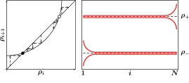
Figure 2: Sketch of possible solutions to recurrence relation (2) on the left and corresponding density profiles on the right. $\rho_{-}$ is a stable fixed point whereas $\rho_{+}$ is unstable.

Upon changing bias $q$ and boundary conditions $\alpha,\gamma$, it is now possible to identify three different phases. For low input rate $\alpha$ at lattice site $N$, the system is in the low density (LD) phase, whereas low growth or release rate $\gamma$ at lattice site 1 leads to the high density (HD) phase. The crossover between low density and high density phase is governed by a first-order transition, where both phases coexist. The locations of the phases as determined by the mean-field theory are similar to the refined $\alpha,\gamma$ phase diagram in fig. 3, which we will discuss below. When both rates $\alpha$ and $\gamma$ are high, the fixed points of eq. (2) do no longer exist and the system is in the maximal current (MC) phase. The density profile is then no longer controlled by the boundary conditions $\alpha$ and $\gamma$. Instead, the bottleneck in the system is given by the bulk dynamics, namely due to the implicit hard-core interaction, which restricts the current or tip speed to its maximum value $J_{MC}=v_{MC}=(3-2\sqrt{2})(q-p)$. It is determined from eq. (3) by setting the root to zero, i.e., when the two fixed points merge. Decreasing the hopping rate bias $q$ below $1$ slows down the bulk dynamics which results in an expanding maximal current phase in the phase diagram.

In order to determine the phases just discussed within the formulated mean-field theory, we extended and generalized the procedure of ref. [17] to $q<1$. We shortly summarize the reasoning. Setting $\rho_{N-1}=\rho_{N}$ in the mean-field rate equation for the boundary on the right,

$$\dot{\rho_{N}}=p(1-\rho_{N})\rho_{N-1}-q(1-\rho_{N-1})\rho_{N}+\alpha(1-\rho_{N})\;,$$ (4)

yields the boundary condition $\rho_{N}=\alpha/(q-p)$. In the LD phase, $\rho_{N}$ equals the stable fixed point $\rho_{-}$ of eq. (3) which gives an expression for the LD current or tip speed $J_{LD}=v_{LD}$. However, the iteration of eq. (2) starting at $\rho_{2}$ only converges to the stable fixed point $\rho_{-}$ if it starts below the unstable fixed point $\rho_{+}$, i.e., if $\rho_{2}<\rho_{+}$. Using the expression for $J_{LD}=v_{LD}$, this condition leads to a phase boundary against the HD phase. In the HD phase the tip velocity $v_{HD}$ and the high density value $\rho_{+}$ follow by setting $\rho_{2}=\rho_{+}$. From $\rho_{2}=\rho_{+}$ the density then has to decay towards $\rho_{N}=\alpha/(q-p)$ at the boundary on the right. This sets up a stationary shock profile at the phase transition between LD and HD phase. Close to this phase transition in the HD phase, the shock moves away from the tip but never reaches the other boundary of the lattice. Only further away from the phase transition, does the high density expand throughout the lattice except in a narrow region close to the boundary on the right.

Monte Carlo simulations of our model were done using a random sequential update where sites are picked randomly one after another and updated according to rates $\alpha,\gamma,q$. One time step consists of updating all $N$ lattice sites. The tip velocity $v$ is then determined as a function of either $\alpha$ or $\gamma$ for a given value of $q$. We localize the HD-MC or LD-MC phase transition when $v$ reaches a constant maximum value which indicates the MC phase. As already indicated, the resulting phase diagram obtained by the mean-field approach does not coincide very well with results from Monte-Carlo simulations. An improved mean-field calculation that takes into account correlations between site $1$ and $2$ by setting $\langle n_{1}n_{2}n_{i}\rangle=\langle n_{1}n_{2}\rangle n_{i}$, predicts a more precise phase diagram. This was already observed for $q=1$, i.e., in the totally asymmetric case [17]. In contrast to the mean-field approach discussed above, iteration of eq. (2) then starts at site $3$ instead of site $2$. In particular, to eliminate $\langle n_{1}n_{2}\rangle$ in the equation for $\rho_{3}$, one needs to evaluate the rate equation for the state $\langle n_{2}(1-n_{1})\rangle$. The resulting phase diagram is shown in fig. 3 and compared to Monte-Carlo simulations. The improved mean-field calculations correctly predict the phase boundaries between LD and MC phases for various $q$ values whereas the boundaries between HD and MC phases still show some deviations from simulations. This was already observed in [17]. Since determining the HD-MC boundary involves the starting value of iteration (2), the result depends strongly on the number of site correlations that are taken into account at the tip. Figures 4(a) and (b) show density profiles at constant $\alpha$, $\gamma$ that convert from the respective LD or HD phase at $q=1$ to the MC phase at $q=0.8$ and 0.6.

For our purposes the main conclusion is that the system reaches a non-equilibrium steady state characterized by a constant current or tip speed $v$. Hence, the lattice grows linearly in time: $N(t)=vt$. This is valid for all three phases and the actual value of $v$ depends on the parameters $\alpha$, $\gamma$ and $q$. With $v_{MC}=(3-2\sqrt{2})(q-p)$ in the MC phase, we obtain

$$N(t)=(3-2\sqrt{2})(q-p)t\;,\qquad q>p\;,$$ (5)

which agrees with simulations [see fig. 6(a)]. Note that Eq. (5) predicts $N(t)\rightarrow 0$ for decreasing bias $q\rightarrow 0.5$. However, Monte-Carlo simulations show a non-vanishing growth of the lattice for $q=p$. So, we have to study this case separately.

Figure 3: Phase diagram of extending TASEP. Monte Carlo simulation (symbols) and improved mean-field calculations (lines) are shown for $q=1.0$, 0.8, and 0.6. Horizontal lines are boundaries between HD and MC phases. Vertical lines separate LD from MC phases. Bullets: parameters of density plots in figs. 4(a), (b).

When $q=p=0.5$, the bulk of the lattice is not driven anymore, i.e., the condition of detailed balance is fulfilled in the bulk but not at the boundaries. The system is still kept out of equilibrium. For $q=p$, eqs. (2) reduce to

$$\left.\begin{array}[]{rl}\rho_{1}={v}/{\gamma},\qquad\rho_{2}=2v+v/\gamma,\\ \\ \rho_{i+1}=\rho_{i}(1+2v)+2v\;,\quad i\geq 2\;.\end{array}\right.$$ (6)

The recurrence relation does not have a fixed point with $\rho>0$ and the density grows to infinity, $\lim_{i\rightarrow\infty}\limits\rho_{i}=\infty$. To bypass this behavior, we impose that the density reaches the physical maximum at the boundary on the right, $\rho_{N}=1$. For $N\gg 1$ and with $\rho_{N}=1$ one readily shows that $\rho_{1}=v/\gamma\ll 1$ and therefore negligible in eqs. (6). Then, the recurrence relation of (6) is solved by

$$\rho_{i}=(1+2v)^{i-1}-1\;.$$ (7)

The condition $\rho_{N}=1$ gives $2=(1+2v)^{N(t)}$, which indicates that $v$ is time-dependent now. By identifying $v(t)$ as ${dN(t)}/{dt}$, we can solve for $N(t)$ and arrive at

$$N(t)=\sqrt{\ln{2}}\sqrt{t}\qquad\mathrm{for}\qquad t\gg 1\;.$$ (8)

This result is confirmed by simulations as indicated in fig. 6(a). It is independent of $\alpha$ and $\gamma$, i.e., the MC phase fills the whole phase diagram. It also shows that the current in the lattice is ohmic, $J=v={dN(t)}/{dt}\propto 1/N(t)$.

We note that the growth function of eq. (8) is consistent with a continuum approach for this particular system. The non-extending TASEP with fixed $N$, open boundaries, and $q=p$ reduces to the diffusion equation in the continuum limit. Hence, to obtain a continuous model of the extending TASEP with $q=p$, one has to formulate the diffusion equation on a growing domain. Similar to writing a reaction-diffusion equation on a growing domain [19], we find [20]

$$\frac{\partial\rho}{\partial t}=\frac{1}{2N(t)^{2}}\frac{\partial^{2}\rho}{\partial x^{2}}-\frac{1}{N(t)}\frac{dN(t)}{dt}\rho,\quad\quad x\in[0,1]\;,$$ (9)

where we replaced $\rho_{i}(t)$ by $\rho(x,t)$ and the growing domain is mapped on the interval $[0,1]$. This equation only has a stationary solution in the case of diffusive growth $N(t)\propto\sqrt{t}$. For $\partial\rho/\partial t=0$ and using growth function (8), we arrive at the time-independent equation

$$\frac{1}{\ln 2}\frac{d^{2}\rho}{dx^{2}}-\rho=0\;.$$ (10)

Under the assumption of Dirichlet boundary conditions $\rho(0)=0$ and $\rho(1)=1$, where the tip of the lattice is located at $x=0$, the stationary solution reads

$$\rho(x)=\frac{\sinh(\sqrt{\ln 2}\,x)}{\sinh\sqrt{\ln 2}}\;.$$ (11)

Monte Carlo simulations confirm this density profile (see fig. 4(c)). The deviation from a linear density profile, i.e., the solution to the non-extending TASEP with $q=p$, is rather small.

Figure 4: Monte Carlo simulations of density profiles for different phases: (a) LD phase with crossover to MC phase ($q=0.8,0.6$), (b) HD phase with crossover to MC phase ($q=0.8,0.6$) [Bullets in fig. 3 give the location in the phase diagram], (c) $q=p$, and (d) $q<p$.

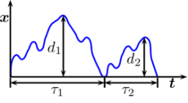
Figure 5: Trajectory of a biased random walker with fixed wall at the origin. The random walker starts at $x=0$. The height of an excursion is called $d_{i}$, the length is called $\tau_{i}$.

When $q<p$, the particles in the bulk prefer to hop to the right, even though the boundary conditions enforce a current from right to left. As a result, the growth function (5) becomes negative indicating that the mean-field calculation is not applicable in this case. Studies of the non-extending TASEP with $q<p$ exist [21, 22] and exact solutions revealed a reverse bias phase where the particle current decreases exponentially with system size $N$. In our case, we expect that the lattice grows very slowly for $q<p$. Furthermore, most of the particles will stay in a domain at the right boundary, whereas near the left boundary most of the sites are vacant. Monte Carlo simulations confirm that there is a domain interface between an empty domain and a ”jammed” domain. As fig. 4(d) shows, this domain wall is roughly located in the middle of the lattice. Now, whenever the left-most particle in the lattice reaches the tip, the lattice will extend by one site. After such a growth event, the next particle in the lattice becomes the left-most particle. Therefore, the growth of the lattice is equivalent to finding the probability that a biased random walker reaches a maximum distance from a bounding wall. In this picture, the wall is given by the domain interface between the empty domain on the left and the ”jammed” domain on the right and the maximum distance is the distance of the lattice tip from the domain interface. Figure 5 depicts a trajectory of a biased random walker with fixed wall at the origin. The random walker is on excursions that last for a timespan of $\tau_{i}$ and have a maximum distance $d_{i}$ from the origin. Ref. [23] determines the probability for $d_{i}$ to be smaller than some threshold $c$ in the long-time limit as

$$P(d_{i}<c)=1-e^{-c/\kappa}\;,$$ (12)

where $\kappa$ characterizes the step-length distribution $W(X_{i})$ of the random walker by the condition

$$\langle e^{X_{i}/\kappa}\rangle=1\;.$$ (13)

In our case, the respective probabilities for hops to the left or right, i.e., away from or towards the origin, are $W(X_{i}=+1)=q$ and $W(X_{i}=-1)=p$. The condition (13) gives

$$qe^{1/\kappa}+pe^{-1/\kappa}=1\;,$$

which results in

$$\kappa=\left(\ln\frac{p}{q}\right)^{-1}\;.$$ (14)

At time $t$ the random walker made $t/\langle\tau_{i}\rangle$ excursions and the maximum $M_{t}$ is given by

$$M_{t}=\mathrm{max}(d_{1},d_{2},\dots,d_{{t}/{\langle\tau_{i}\rangle}})\;.$$ (15)

The probability that $M_{t}<c$ becomes

$$P(M_{t}<c) = P(d_{1}<c)\cdot P(d_{2}<c)\dots P(d_{t/\langle\tau_{i}\rangle}<c)$$

$$= \left(1-e^{-c/\kappa}\right)^{t/\langle\tau_{i}\rangle}\;.$$

Replacing $c$ by $c+\kappa\ln t$ yields

$$P(M_{t}<c+\kappa\ln t)=\left(1-\frac{e^{-c/\kappa}}{t}\right)^{{t}/{\langle\tau_{i}\rangle}}\;$$ (16)

and in the limit of large $t/\langle\tau_{i}\rangle$, one obtains the Gumbel distribution [24]

$$P(M_{t}<c+\kappa\ln t)=\exp(-e^{-c/\kappa}/\langle\tau_{i}\rangle)\;.$$ (17)

This means that the probability for a maximum excursion stays constant in time, when in the long-time limit the maximum grows as

$$M_{t}=\kappa\ln t+c\;,$$ (18)

where $c$ is an undetermined constant. Since the domain interface is situated approximately in the middle of the lattice, the growth function of the whole lattice is then

$$N(t)=2\left(\ln\frac{p}{q}\right)^{-1}\ln t+c\;,\qquad\qquad q<p\;,$$ (19)

with tip speed

$$v=\frac{dN(t)}{dt}\propto\exp(-\frac{N}{2\kappa})\;.$$ (20)

Interestingly, the dependence of $v$ on $N$ agrees qualitatively with the dependence of the current on $N$ in the non-extending TASEP with negative drift [21, 22].

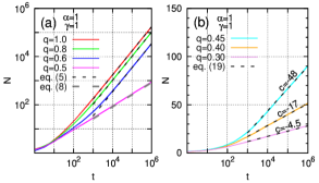
Figure 6: Lattice growth determined from Monte Carlo simulations. (a) Upper 3 curves: positive drift with $q>p$, bottom curve: no drift with $q=p=0.5$. (b) Negative drift with $q<p$.

Simulations of an extending lattice for different $q<0.5$ agree very well with this theory by reproducing the logarithmic growth law (19) with its prefactor $2\kappa$ [see fig. 6(b)]. This is even true for $q$ approaching 0.5 when the domain interface in fig. 4(d) becomes broader and, strictly speaking, the bounding wall of our model does not exhibit a hard-core repulsion for the random walker. Just as in the $q=p$ case, simulations of an extending lattice are independent of $\alpha$ and $\gamma$. Note that the analogy with a biased random walker bounded by a wall also gives the growth laws $N(t)\propto t$ for $q>p$ and $N(t)\propto\sqrt{t}$ for $q=p$. We checked this by Monte-Carlo simulations.

Figure 7: Lattice growth speed from simulations for small negative bias ($q=0.4999$). The inset shows flagellar elongation data of three samples of Salmonella and fits, taken from [3].

Summarizing our results, we found three distinct regimes for the bias $q$ in the extending TASEP with qualitatively different growth functions. The experimental observation of logarithmic growth for flagellar filaments [3] mentioned in the introduction is in qualitative agreement with our model when the drift is negative ($q<0.5$). In order to compare our result with the experiment in more detail, we carried out simulations with very small negative drift. By setting $q=0.4999$, it was possible to achieve a lattice length of the order of $N=20000$ in reasonable simulation time while still reaching the logarithmic growth regime. If each growth event mimics one flagellin molecule, $N=20000$ corresponds to a filament of about $10\mu m$. For our estimate, we used the length $55\mathring{A}$ for a flagellin molecule and the fact that 11 flagellin molecules make up the circular cross section of the hollow flagellar filament. The speed of elongation of flagellar filaments in the experiment was found to decrease exponentially with increasing length for filament lengths in the range from $4$ to $14\mathrm{\mu m}$ (see inset of fig. 7) [3]. This is in agreement with our simulations as illustrated in fig. 7. However, it remains to establish an explanation why the flagellin in the hollow filament should exhibit a negative drift towards the cell body. It has been suggested that proton motive force (PMF) is biasing the Brownian motion of the flagellin translocation process [25]. The details of this mechanism are, however, very unclear at this stage and should be subject to further research.

References

- [1] \NameBerg H. C. \BookE. coli in Motion \PublSpringer, New York \Year2004.
- [2] \NameKeener J. P. \REVIEWBull. Math. Biol.6820061761.
- [3] \NameIino T. \REVIEWJ. Supramol. Struct.21974372.
- [4] \NameDerrida B., Domany E. Mukamel D. \REVIEWJ. Stat. Phys691992667.
- [5] \NameDerrida B., Evans M. R., Hakim V. Pasquier V. \REVIEWJ. Phys. A: Math. Gen.2619931493.
- [6] \NameSchütz G. Domany E. \REVIEWJ. Stat. Phys.721993277.
- [7] \NameKrug J. \REVIEWPhys. Rev. Lett.6719911882.
- [8] \NameParmeggiani A., Franosch T. Frey E. \REVIEWPhys. Rev. Lett.902003086601.
- [9] \NameMukamel D. \BookSoft and Fragile Matter: Nonequilibrium Dynamics, Metastability and Flow \EditorCates M. E. Evans M. R. \PublTaylor & Francis \Year2000 \Pages237258.
- [10] \NameMacDonald C. T., Gibbs J. H. Pipkin A. C. \REVIEWBiopolymers619681.
- [11] \NameFrey E., Parmeggiani A. Franosch T. \REVIEWGenome Informatics15200446.
- [12] \NameBarlovic R., Santen L., Schadschneider A. Schreckenberg M. \REVIEWEur. Phys. J. B51998793.
- [13] \NameChowdhury D., Santen L. Schadschneider A. \REVIEWPhys. Rep3292000199.
- [14] \NameNowak S. A., Fok P. W. Chou T. \REVIEWPhys. Rev. E762007031135.
- [15] \NameDorosz S., Mukherjee S. Platini T. \REVIEWPhys. Rev. E812010042101.
- [16] \NameKwon H. W. Choi M. Y. \REVIEWPhys. Rev. E822010013101.
- [17] \NameSugden K. E. P. Evans M. R. \REVIEWJ. Stat. Mech2007P11013.
- [18] \NameSugden K. E. P., Evans M. R., Poon W. C. K. Read N. D. \REVIEWPhys. Rev. E752007031909.
- [19] \NameCrampin E. J., Gaffney E. A. Maini P. K. \REVIEWBull. Math. Biol.6119991093.
- [20] \NameSchmitt M. \BookA growth model for bacterial flagella \Publdiploma thesis, Technische Universität Berlin \Year2010. \revision
- [21] \NameBlythe R. A., Evans M. R., Colaiori F. Essler F. H. L. \REVIEWJ. Phys. A: Math. Gen.3320002313. \revision
- [22] \NameDe Gier J., Finn C. Sorrell M. \REVIEWarXiv20111107.2744v1 [cond-mat.stat-mech].
- [23] \NameIglehart D. L. \REVIEWAnnals Math. Stat.431972627.
- [24] \NameGumbel E. J. \BookStatistical theory of extreme values and some practical applications \Vol33 \PublU.S. National Bureau of Standards Applied Mathematics Series, Washington, DC \Year1954.
- [25] \NameMinamino T., Imada K. Namba K. \REVIEWMol. BioSyst.420081105.