Spatio-temporal behaviour of the deep chlorophyll maximum in Mediterranean Sea: Development of a stochastic model for picophytoplankton dynamics

Abstract

In this paper, by using a stochastic reaction-diffusion-taxis model, we analyze the picophytoplankton dynamics in the basin of the Mediterranean Sea, characterized by poorly mixed waters. The model includes intraspecific competition of picophytoplankton for light and nutrients. The multiplicative noise sources present in the model account for random fluctuations of environmental variables. Phytoplankton distributions obtained from the model show a good agreement with experimental data sampled in two different sites of the Sicily Channel. The results could be extended to analyze data collected in different sites of the Mediterranean Sea and to devise predictive models for phytoplankton dynamics in oligotrophic waters.

I Introduction

Natural systems are characterized by two factors: (i) non-linear interactions among their parts; (ii) external perturbations, both deterministic and random, coming from the environment (Spagnolo et al., 2004; Huppert et al., 2005; Ebeling and Spagnolo, 2005; Provata et al., 2008; Spagnolo and Dubkov, 2008; Valenti et al., 2008). It is worth noting that natural systems, because of these characteristics, are complex systems (Grenfell et al., 1998; Zimmer, 1999; Bjørnstad and Grenfell, 2001; Spagnolo et al., 2002; La Barbera and Spagnolo, 2002; Spagnolo and La Barbera, 2002; Spagnolo et al., 2003, 2005; Caruso et al., 2005; Chichigina et al., 2005; Fiasconaro et al., 2006; Valenti et al., 2006; Chichigina, 2008). Therefore, the study of a marine ecosystem has to be performed by considering the perturbations, not only deterministic but also random, due to the fluctuations of the environmental variables. This implies the necessity of including in the model a term which describes the continuous interaction between the ecosystem and environment. In particular, physical variables, such as temperature, salinity and velocity field, are affected by random perturbations and can be therefore treated as noise sources. This causes the phytoplankton behaviour to be subject to a stochastic dynamics, and allows to expect that a stochastic approach should reproduce the distributions of phytoplankton biomass better than deterministic models. On this basis, noise effects have to be included to better analyze the dynamics of a marine system such as that studied in this work.
The growth of phytoplankton is limited by the concentration of nutrients $R$ and intensity of light $I$ (Klausmeier and Litchman, 2001; Klausmeier et al., 2007). In particular, the survivance of phytoplankton is strictly connected with the presence of sufficiently high nutrient concentration. It is worth stressing that nutrients, which are in solution, diffuse from the bottom (seabed) towards the top (water surface). Nutrient distributions along the water column are therefore characterized by an increasing trend from the sea surface to the benthic layer. As a consequence, the positive gradient of nutrient concentration causes the maxima of chlorophyll, which is contained in the phytoplankton cells, to be localized in deep subsurface layers. This condition constitutes one of the most striking feature of the nutrient poor waters in ocean ecosystems and freshwater lakes (Anderson, 1969; Cullen, 1982; Abbott et al., 1984; Tittel et al., 2003). Conversely, the light penetrates through the surface of the water and has an exponentially decreasing trend along the water column. This characteristic makes the deep layers unfavourable for the photosynthesis, determining, as a consequence, adverse life conditions for phytoplankton. In particular, light is a crucial parameter for the localization of the deep chlorophyll maximum (DCM), as revealed by the significant correlation found between the depth of DCM and light intensity over the Mediterranean basin in summer (Brunet et al., unpublished data).
The dynamics, competition and structuring of phytoplankton populations have been investigated in a series of theoretical studies based on model systems (Radach and Maier-Reimer, 1975; Varela et al., 1992; Huisman and Weissing, 1995; Klausmeier and Litchman, 2001; Diehl, 2002; Hodges and Rudnick, 2004; Beckmann and Hense, 2007; Klausmeier et al., 2007; Mei et al., 2009; Bougaran et al., 2010). In a few recent investigations it was observed that in the presence of an upper mixed layer either surface or deep maxima can be observed indifferently under almost the same conditions (Venrick, 1993; Holm-Hansen and Hewes, 2004; Ryabov et al., 2010).
In view of analyzing an ecological system, as a preliminary step it is necessary to define the correct values of the parameters and the role that they play on the dynamics of the populations, specifically when the coexistence of different species in the same community is considered (Norberg, 2004). The responses of the species to environmental solicitations strongly depend on the biological and physical parameters. Among these, a relevant role is played by the phytoplankton velocity which is strictly connected with the microorganism size, one of the main functional traits for phytoplankton diversity. Other parameters that influence the balance of a marine ecosystem are, for example, growth rates and nutrient uptake (Fogg, 1991; Prézelin et al., 1991).
In this paper we deal with data obtained in a hydrologically stable area of the Mediterranean Sea, where the environmental light and nutrients, specifically phosphorus, contribute to determine life conditions. The Mediterranean basin is characterized by oligotrophic conditions and it has been suggested that there is a decreasing trend over time in chlorophyll concentration. This has been associated with increased nutrient limitation resulting from reduced vertical mixing due to a more stable stratification of the basin, in line with the general warming of the Mediterranean  (Barale et al., 2008). Here we consider the Strait of Sicily, which is known to govern the exchanges between the eastern and western basins and is characterized by active mesoscale dynamics (Lermusiaux and Robinson, 2001), strongly influencing the ecology of phytoplankton communities. Moreover, the Strait of Sicily is a biologically rich area of the Mediterranean Sea with a key role in terms of fisheries (Lafuente et al., 2002; Cuttitta et al., 2003). The anchovy growth (along with phytoplankton biomass) in the Sicilian Channel resulted to be mainly explained by changes in the chlorophyll concentration, used as a phytoplankton biomass indicator (Basilone et al., 2004). Our study is performed using a stochastic model obtained by modifying a deterministic reaction-diffusion-taxis model. Specifically, the analysis focuses on the spatio-temporal dynamics of the phytoplankton biomass, and provides the time evolution of biomass concentration along the water column. Finally, the results are compared with experimental data collected in two different sites of the Strait of Sicily.

II Materials and methods

II.1 Environmental data

The experimental data were collected in the period 12^th - 24^th August 2006 in the Sicily Channel area (Fig. 1) during the MedSudMed-06 Oceanographic Survey onboard the R/V Urania. Hydrological data were obtained using a SBE911 plus CTD probe (Sea-Bird Inc.); chlorophyll a fluorescence data (chl a, $\mu$g/l) were contemporary acquired by means of the Chelsea Aqua 3 sensor. In the Libyan area the CTD stations were located on a grid of 12 x 12 nautical miles. Moreover, CTD data have been collected along a transect between the Sicilian and the Libyan coasts. In the present work, two stations out of the whole data set were considered. The selected stations were located on the south of Malta (site L1105) and on the Libyan continental shelf (site L1129b).

Figure 1: Locations of the CTD stations where the experimental data were collected.

The collected data were quality-checked and processed following the MODB instructions (Brankart, 1994) using Seasoft software. The post-processing procedure generated a text file for each station where the values of the oceanographic parameters were estimated with a 1 m step. Hydrological conditions remained constant for the entire sampling period and were representative of the oligotrophic Mediterranean Sea in summer. Nitrate, nitrite, silicate and phosphate concentrations were not determined.

II.2 Phytoplanktonic data

Depending on size the phytoplankton species can be divide into two main fraction:

• $<3\mu m$ picophytoplankton, formed by groups, Prochlorococcus, Synechococcus and picoeukaryotes (Olson et al., 1993; Brunet et al., 2008). This size of phytoplankton accounts for about 80% of the total chl a on average  (Brunet et al., 2006), ranging from 40% to 90% (69% in the DCM) (Brunet et al., 2007).

• $>3\mu m$ nano- and micro-phytoplankton, characterized by a lower correlation with nutrients and salinity respect to picophytoplankton. This is connected with the fact that the contribution of picophytoplankton in the DCM is higher than in the surface layer (Brunet et al., 2006). This larger size fraction of phytoplankton amounts to 20% of the total chl a on average and is uniformly distributed along the water column.

The high pigment diversity of the smaller phytoplankton in the DCM and its elevated contribution to the total chl a indicated a strong degree of adaptation to the quantity and quality of light available (Dimier et al., 2007; Brunet et al., 2008; Dimier et al., 2009a). This is not true for the larger phytoplankton, which is represented mainly by diatoms or Haptophytes. Picoeukaryotes, which belong to the smaller size class, present peculiar eco-physiological properties (Raven et al., 2005; Dimier et al., 2007; Worden and Not, 2008), such as low sinking, high growth rate and low nutrient uptake. Their small size leads to a low package effect, which contributes to the light-saturated rate of photosynthesis that can be achieved at relatively low irradiances (Raven, 1998; Brunet et al., 2003; Raven et al., 2005; Finkel and Irwin, 2005). Due to their peculiarities and relevant role in ecosystem functioning, they constitute a key-group to be considered within a model of population dynamics. In Sicily Channel (Casotti et al., 2003; Brunet et al., 2006, 2007), picophytoplankton is numerically dominated by the Prochlorococcus fraction. In this area the number of Prochlorococcus cells is constant in the first $20$ m, and is characterized in the DCM by an average value of $5.2\times 10^{4}$ cell ml^-1. Average picoeukaryote concentration in the DCM is $0.6\pm 0.4\times 10^{3}$ cell ml^-1, and the mean value of chl a cell^-1 ranges between 10 and 660 fg chl a cell^-1 along the water column, with a significant exponential increase with depth (see Fig. 2) (Brunet et al., 2007). The concentration of chl a (fg cell^-1) per cell in picoeukaryotes was highly variable among different water masses, with significantly higher values in the DCM respect to the surface, as a result of photoacclimation to decreased light irradiances (Brunet et al., 2003; Dimier et al., 2007; Brunet et al., 2008; Dimier et al., 2009a).

Figure 2: Mean vertical profile of chl a per picoeukaryote cell (fg cell^-1). Error bars are Standard Deviation. Equation and $r^{2}$ for the fit are reported on the plots. (Courtesy of Brunet et al., 2007).

III Experimental results

Data obtained from the cruises in two different sites of the Strait of Sicily both for temperature and chl a concentration are shown in Fig. 3.

Figure 3: Profiles of temperature (panels a, c) and chl a concentration (panels b, d) measured in sites L1129b and L1105. The black lines have been obtained by connecting the experimental points corresponding to samples distanced of 1 meter along the water column. The total number of samples measured in the two sites is $n=176$ for L1129b, and $n=563$ for L1105.

In site L1129b, the behaviour of the temperature along the water column indicates the presence of a mixed layer (from the surface to 28 m depth) characterized by a high value of temperature. Below the thermocline (28 m depth) the temperature decreases up to 80 m, becoming uniform below this depth (Fig. 3a). The site L1105 shows a mixed layer over the first 24 m of depth, and a sharp decrease of temperature from 24 to 75 m (Fig. 3c). Experimental data for chl a concentration show a nonmonotonic behaviour, as a function of the depth, characterized by the presence of DCM in both sites (see Fig. 3b,d). Specifically, fluorescence profiles show a similar behaviour in the two sites, with chl a concentration ranging between $0.010$ and $0.17\mu g$ chl a l^-1. Differences between the two sites are observed in the depth, shape and width of the DCM.

IV The Model

In this study we analyze the spatio-temporal dynamics of a picophytoplankton community, limited by nutrient and light in a vertical poorly mixed water column. The mechanism, responsible for the phytoplankton dynamics, is schematically shown in Fig. 4.

Figure 4: (Color online) Scheme of the mechanism responsible for the phytoplankton dynamics (modified from original figure by A. Ryabov). (a) Image of Micromonas NOUM17 (courtesy of Augustin Engman, Rory Welsh, and Alexandra Worden.

The mathematical tool used to simulate the phytoplankton dynamics is an advection-reaction-diffusion model. In particular, we investigate the distribution of the picophytoplankton along the water column, with light intensity decreasing and nutrient concentration increasing with depth. Analysis and numerical elaborations are divided in two phases:

• Phase 1. By using a model based on two differential equations, the distribution of picophytoplankton biomass $b$ is obtained along the poorly mixed water column as a function of the time and depth, and simultaneously the distribution of nutrient concentration $R$, which limits the growth of phytoplankton, is calculated. The results obtained are compared with the experimental data collected in the two different sites of the Strait of Sicily.

• Phase 2. In order to match better the results for $b$ and $R$ to the experimental data, the random fluctuations of the environmental variables are taken into account. In particular, a stochastic model is obtained from the deterministic one by inserting into the equations terms of multiplicative Gaussian noise.

IV.1 The deterministic model

Here we introduce the model consisting of a system of differential equations, with partial derivatives in time and space (depth). The model allows to obtain the dynamics of the phytoplankton biomass $b(z,t)$ and nutrient concentration $R(z,t)$. The light intensity $I(z,t)$ is given by a function varying, along the water column, with the depth and biomass concentration. The behaviour of the phytoplankton biomass, along the water column, is the results of three processes: growth, loss, and movement. The phytoplankton growth rate depends on $I$ and $R$ (Klausmeier and Litchman, 2001; Klausmeier et al., 2007; Mei et al., 2009; Bougaran et al., 2010; Ryabov et al., 2010). The limitation in phytoplankton growth is described by the Monod kinetics (Turpin, 1988). The gross phytoplankton growth rate per capita is given by $\min\{f_{I}(I),f_{R}(R)\}$, where $f_{I}(I)$ and $f_{R}(R)$ are obtained by the Michaelis-Menten formulas

$$f_{I}(I)=rI/(I+K_{I}),$$ (1)

$$f_{R}(R)=rR/(R+K_{R}).$$ (2)

In Eqs. (1), (2), $r$ is the maximum growth rate, while $K_{I}$ and $K_{R}$ are the half-saturation constants for light intensity and nutrient concentration, respectively. Varying $K_{R}$ and $K_{I}$ allows to model, for instance, a species which is better adapted to the light (smaller values of $K_{I}$) or nutrient (smaller values of $K_{R}$). More specifically, we consider a species with small $K_{I}$ and large $K_{R}$ that corresponds to good life conditions at large depth. These constants depend on the metabolism of the specific microorganism considered.
The biomass loss, connected with respiration, death, and grazing, occurs at a rate $m$ (Klausmeier and Litchman, 2001; Huisman et al., 2006; Ryabov et al., 2010). The gross per capita growth rate is defined as

$$g(z,t)=\min(f_{R}(R(z,t)),f_{I}(I(z,t))).$$ (3)

Turbulence, responsible for passive movement of the phytoplankton, is modeled by eddy diffusion. Specifically, we describe turbulence assuming that the vertical diffusion coefficient is uniform with the depth and characterized by a low value ($D_{b}=D_{R}=0.5$). This choice is motivated by the fact that in sites L1129b and L1105 the phytoplankton peaks, located at 87 m and 111 m respectively, are quite far from the thermocline (see Fig. 3). Therefore, phytoplankton should go up (or down) if the biological conditions are more suitable for growth above (below) than below (above). Finally, no migration should occur if the biomass concentrations are the same at different depths. These assumptions about growth, loss, and movement, allow to obtain the following differential equation for the dynamics of biomass concentration $b$ (Klausmeier and Litchman, 2001; Huisman et al., 2006):

$$\frac{\partial b(z,t)}{\partial t}=g(z,t)b(z,t)-mb(z,t)+D_{b}\frac{\partial^{2}b(z,t)}{\partial z^{2}}-v\frac{\partial b(z,t)}{\partial z}.$$ (4)

The positive phytoplankton velocity v, due to active movement, is oriented downward (sinking), in the direction of positive z. Phytoplankton does not enter or leave the water column. This is set by using no-flux boundary conditions at $z=0$ and $z=z_{b}$:

$$\left.\left[D_{b}\frac{\partial b}{\partial z}-vb\right]\right|_{z=0}=\left.\left[D_{b}\frac{\partial b}{\partial z}-vb\right]\right|_{z=z_{b}}=0.$$ (5)

Eddy diffusion is responsible for mixing of the nutrient concentration along the water column, with diffusion coefficient $D_{R}$. The nutrient consumed by the phytoplankton is also obtained from recycled dead phytoplanktonic microorganisms. The dynamics of nutrient concentration can be therefore modeled as follows:

$$\frac{\partial R(z,t)}{\partial t}=-\frac{b(z,t)}{Y}g(z,t)+D_{R}\frac{\partial^{2}R(z,t)}{\partial z^{2}}+\varepsilon m\frac{b(z,t)}{Y},$$ (6)

Here $Y$ is the phytoplankton produced biomass per unit of consumed nutrient, and $\varepsilon$ is the nutrient recycle coefficient. Since the nutrient is not supplied by the sea surface but comes from the seabed, its concentration is set to the constant value $R_{in}$ in the sediment and, as a consequence, to the value $R(z_{b})$ in the bottom of the water column. In fact the nutrient diffuses across the sediment-water interface with a rate proportional to the concentration difference between the solid phase (seabed) and the deepest water layer (bottom of the water column). Accordingly, the boundary conditions are given by:

$$\left.\frac{\partial R}{\partial z}\right|_{z=0}=0,\quad\left.\frac{\partial R}{\partial z}\right|_{z=z_{b}}=h(R_{in}-R(z_{b})),$$ (7)

where $h$ is the permeability of the interface. Finally, taking into account Lamber-Beer’s law (Shigesada and Okubo, 1981; Kirk, 1994), the light intensity is characterized by an exponential decrease modeled as follows:

$$I(z)=I_{in}\exp\left\{-\int_{0}^{z}\left[ab(Z)+a_{bg}\right]dZ\right\},$$ (8)

where $a$ and and $a_{bg}$ are phytoplankton biomass and background attenuation coefficients, respectively. Equations (4)-(8) form the biophysical model used in our study.

IV.2 Results of the deterministic model

The time evolution of the system is studied by analyzing the spatio-temporal dynamics of biomass and nutrient concentrations. In particular, by using a numerical method, implemented by a program in C++ language and based on an explicit finite difference scheme, equations (4)-(8) are solved. The increment of the spatial variable is set to 0.5 m. In view of reproducing the spatial distributions observed in the real data for the phytoplankton biomass (see Fig. 3), we choose the values of the environmental and biological parameters to satisfy the monostability condition corresponding to the presence of a deep chlorophyll maximum (Klausmeier and Litchman, 2001; Huisman et al., 2006; Ryabov et al., 2010). The numerical values assigned to the parameters are shown in Table 1.

Table 1: Parameters used in the model. The values of the biological and environmental parameters are those typical of picophytoplankton and summer period in Mediterranean Sea, respectively.

Specifically, the values of the biological parameters $r$, $K_{I}$, $K_{R}$, $v$, have been chosen to reproduce the behaviour of picoeukaryotes. We note that, in systems characterized by a constant value of the diffusion coefficient, the stationary state does not depend on the initial conditions, according to previous studies (Klausmeier and Litchman, 2001; Ryabov et al., 2010). In order to obtain the steady spatial distribution, we integrated numerically our equations over a time interval long enough to observe the stationary solution. As initial conditions we consider that the phytoplankton biomass is concentrated in the layer where the maximum of the experimental chlorophyll distribution is observed. On the other side the nutrient concentration is approximately constant from the water surface to the DCM, and increases linearly below this point up to the seabed.
Preliminary analysis (data not shown) revealed that the stationary solution is characterized by DCMs which are shallower as the nutrient supply increases, and deeper for enhanced light radiation. In general, large values of $I_{in}$ (incident light intensity at the water surface) lead to stationary conditions characterized by DCM, while large values of $R_{in}$ (nutrient concentration in the sediment) determine an upper chlorophyll maximum (UCM). Finally, for intermediate values of $I_{in}$ and $R_{in}$ the chlorophyll maximum can be localized close to the surface or at different depths, depending on the values of the other parameters (Ryabov et al., 2010).
In our study the values of the light intensity resulted to be quite high in both sites, since sampling occured during summer (August 2006). In this period the light intensity at the water surface is larger than $1300$ $\mu$mol photons m^-2 s^-1. Moreover the sinking velocity is set to the value typical for picophytoplankton, $v=0.1$ m day^-1 (Huisman et al., 2006). The diffusion coefficent is fixed at the value $D_{b}=0.5$ cm² sec^-1, which corresponds to the condition of poorly mixed waters. By solving Eqs. (4)-(8) we obtain the biomass concentration expressed in cells/m³ along the water column. Depths of the water column used in the model were set according to the measured depths in the corresponding marine sites. Moreover the light intensities, $I_{in}$, are fixed using data available on the NASA web site. Finally, nutrient concentrations at the seabed were set at values such as to obtain, for each site, a peak of biomass concentration at the same position of the peak experimentally observed. All the other parameters are the same in both sites. The growth rate obtained from Eq. (3) agrees with the values measured by other authors (Dimier et al., 2009b).
We note that our numerical results were obtained using a maximum simulation time $t_{max}=10^{5}~{}h$. Simulations (here not reported) performed within the deterministic approach show that the stationary regime is reached at $t\approx 3\cdot 10^{4}~{}h$. This indicates that, to reach the steady state, it is sufficient to solve the equations of our model with a maximum time $t_{max}=4\cdot 10^{4}~{}h$. By this way, we get the stationary profiles, both for biomass concentration and light intensity, shown in Fig. 5. Here we can note the presence of a biomass peak as found in the experimental data, and the typical exponential behaviour of the light intensity.

Figure 5: Stationary distributions of the biomass concentration and light intensity in sites L1129b (panels a, b) and L1105 (panels c, d) as a function of depth.

Figure 6: (Color online). Stationary distribution of the chlorophyll a concentration as a function of depth calculated (red line) by the deterministic model and measured (green line) in sites (a) L1129b and (b) L1105.

To compare the theoretical results with the experimental data, we exploit the curve of Fig. 2 to convert the cell concentrations, obtained from the model and expressed in cell/m³, into chl a concentrations expressed in $\mu$g/l. We recall that about 43% of the total quantity of chl a (Huisman et al., 2006; Brunet et al., 2006) is due to nano- and micro-phytoplankton (20% of the total chl a on average), and Synechococcus (23% of the total chl a on average), quite uniformly distributed along the water column. Since our model accounts for the dynamics of picoeukaryotes, to compare the numerical results with the experimental data, we consider the 43% of the total biomass and divide it by depth, obtaining for each site the value $\Delta b_{chl\thinspace a}$, which represents a constant concentration due to other phytoplankton species present in the water column. Finally along the water column we add the theoretical concentration with $\Delta b_{chl\thinspace a}$ and obtain, for the distributions of chl a concentration, the stationary theoretical profiles consistent with those of the experimental data. The results are shown in Fig. 6. Here we can observe that in both sites the deep chlorophyll maxima obtained from the model are located at the same depth of those observed experimentally. However, the shape of the theoretical chl a distributions is quite different from the experimental profiles. Finally, we note that in site L1105 the magnitude of the theoretical DCM is significantly different from that observed in real data.

IV.3 The Stochastic Model

In the previous section we used a deterministic model to fit the experimental distributions of chl a concentration. The results obtained reproduce partially the characteristics of the experimental profiles. In order to get a good agreement between real data and theoretical results, we recall that the sea is a complex system. This implies, as discussed in Introduction, the presence of non-linear interactions among its parts (Spagnolo et al., 2004; Huppert et al., 2005; Ebeling and Spagnolo, 2005; Provata et al., 2008; Spagnolo and Dubkov, 2008; Valenti et al., 2008) and a continuous interaction between the ecosystem and environment. In particular, the system dynamics is affected not only by deterministic forces but also random perturbations coming from the environment. In this context environmental variables, due to their random fluctuations, can act as noise sources, causing phytoplankton to be subject to a stochastic dynamics. Therefore, in order to perform an analysis that takes account for real conditions of the ecosystem, it is necessary to modify our model, including the noise effects. In the following we analyze two different situations.
Case 1. The environmental noise affects only the biomass concentration. Therefore, Eqs. (5)-(8) are maintained unaltered, while Eq. (4) becomes

$$\frac{\partial b}{\partial t}=gb-mb+D_{b}\frac{\partial^{2}b}{\partial z^{2}}-v\frac{\partial b}{\partial z}+b\thinspace\xi_{b}(z,t)$$ (9)

Case 2. The environmental noise affects only the nutrient concentration. In this case, Eqs. (4),(5),(7),(8) are maintained unaltered, while Eq. (6) is replaced by

$$\frac{\partial R}{\partial t}=[m\varepsilon-g]\frac{b}{Y}+D_{R}\frac{\partial^{2}R}{\partial z^{2}}+R\thinspace\xi_{R}(z,t).$$ (10)

In Eqs. (9) and (10), $\xi_{b}(z,t)$ and $\xi_{R}(z,t)$ are statically independent white Gaussian noises with the usual properties $\langle\xi_{b}(z,t)\rangle=0$, $\langle\xi_{R}(z,t)\rangle=0$, $\langle\xi_{b}(z,t)\xi_{b}(z^{\prime},t^{\prime})\rangle=\sigma_{b}\delta(z-z^{\prime})\delta(t-t^{\prime})$, $\langle\xi_{R}(z,t)\xi_{R}(z^{\prime},t^{\prime})\rangle=\sigma_{R}\delta(z-z^{\prime})\delta(t-t^{\prime})$, where $\sigma_{b}$ and $\sigma_{R}$, are the noise intensities. We note that the two noise sources are spatially uncorrelated, that is at the generic point $z$ no effects is present due to random fluctuations occurring in $z^{\prime}\neq z$.

IV.4 Results of the stochastic model

In this paragraph we solve numerically, within the Ito scheme, the equations of the stochastic model for different values of the noise intensities, obtaining the distributions of the picophytoplankton concentration as an average over $1000$ realizations. We recall that the ecosystem is characterized by non-linear interactions among its parts. Because of this feature the response of the system to external solicitations is also non-linear. Therefore, one can not expect that the presence of a symmetric noise with zero mean, i.e. Gaussian noise used in the model, produces in average the same effect as a deterministic dynamics (Giuffrida et al., 2009). On the other side, the use of a random function, i.e. noise source, to simulate the spatio-temporal behaviour of the system, makes the single realization unpredictable and unique, and therefore non-representative of the real dynamics. As a consequence, one possible choice to describe correctly the time evolution of the system is to calculate the average of several realizations. This procedure, indeed, allows to take into account different ”trajectories” obtained by the integration of the stochastic equations, without focusing on a specific realization (Spagnolo et al., 2004). According to the discussion of Paragraph IV.2, we calculated the solutions for a maximum simulation time $t_{max}=4\cdot 10^{4}~{}h$. In Figs. 7 and 8 we show the results for case 1.

Figure 7: (Color online). Average chl a concentration calculated (red line) for different values of $\sigma_{b}$ by the stochastic model (case 1, see Eqs. (5), (6), (7), (8), (9)) as a function of depth. Results are compared with chl a distributions measured (green line) in site L1129b. The theoretical values were obtained averaging over $1000$ numerical realizations. The values of the parameters are those shown in Table 1. The noise intensities are: (a) $\sigma_{b}=0$ (deterministic case), (b) $\sigma_{b}=0.10$, (c) $\sigma_{b}=0.20$, (d) $\sigma_{b}=0.22$, (e) $\sigma_{b}=0.25$ and (f) $\sigma_{b}=0.30$.

Figure 8: (Color online). Average chl a concentration calculated (red line) for different values of $\sigma_{b}$ by the stochastic model (case 1, see Eqs. (5), (6), (7), (8), (9)) as a function of depth. Results are compared with chl a distributions measured (green line) in site L1105. The theoretical values were obtained averaging over $1000$ numerical realizations. The values of the parameters are those shown in Table 1. The noise intensities are: (a) $\sigma_{b}=0$ (deterministic case), (b) $\sigma_{b}=0.05$, (c) $\sigma_{b}=0.10$, (d) $\sigma_{b}=0.15$, (e) $\sigma_{b}=0.20$ and (f) $\sigma_{b}=0.30$.

Here we note that, in both sites, for higher noise intensities the peaks of the two average chl a distributions show: (i) a decrease of their magnitude; (ii) a small displacement along the water column. For suitable values of the noise intensity the peaks of the average chl a distributions obtained from the model match very well the experimental data. We note also that the two DCMs are located at 90 m (site L1129b) and 106 m (site L1105) of depth (in Figs. 7d and 8d compare theoretical (red line) and experimental (green line) profiles).

Table 2: Results of $\chi^{2}$, reduced chi-square ($\tilde{\chi}^{2}$) goodness-of-fit test for site L1129b (left panel) and site L1105 (right panel) for different values of $\sigma_{b}$ (stochastic dynamics - case 1). The number of samples along the water column is n = 176 for site L1129b and n = 563 for site L1105.

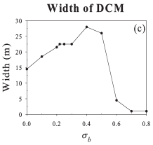
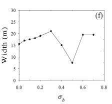
Figure 9: Magnitude, depth, and width of the DCM as a function of $\sigma_{b}$ obtained from the model for site L1129b (panels a, b, c) and site L1105 (panels d, e, f).

Figure 10: (Color online). Average chl a concentration calculated (red line) for different values of $\sigma_{R}$ by the stochastic model (case 2, see Eqs. (4), (5), (7), (8), (10)) as a function of depth. Results are compared with chl a distributions measured (green line) in site L1129b. The theoretical values were obtained averaging over $1000$ numerical realizations. The values of the parameters are those shown in Table 1. The noise intensities are: (a) $\sigma_{R}=0$ (deterministic case), (b) $\sigma_{R}=0.0010$, (c) $\sigma_{R}=0.0015$, (d) $\sigma_{R}=0.0020$, (e) $\sigma_{R}=0.0025$ and (f) $\sigma_{R}=0.0050$.

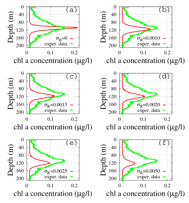
Figure 11: (Color online). Average chl a concentration calculated (red line) for different values of $\sigma_{R}$ by the stochastic model (case 2, see Eqs. (4), (5), (7), (8), (10)) as a function of depth. Results are compared with chl a distributions measured (green line) in site L1105. The theoretical values were obtained averaging over $1000$ numerical realizations. The values of the parameters are those shown in Table 1. The noise intensities are: (a) $\sigma_{R}=0$ (deterministic case), (b) $\sigma_{R}=0.0010$, (c) $\sigma_{R}=0.0015$, (d) $\sigma_{R}=0.0020$, (e) $\sigma_{R}=0.0025$ and (f) $\sigma_{R}=0.0050$.

Table 3: Results of $\chi^{2}$, reduced chi-square ($\tilde{\chi}^{2}$) goodness-of-fit test for site L1129b (left panel) and site L1105 (right panel) for different values of $\sigma_{R}$ (stochastic dynamics - case 2). The number of samples along the water column is n = 176 for site L1129b and n = 563 for site L1105.

To better understand the dependence of the biomass concentration on the random fluctuations of the nutrient, according to the procedure followed for case 1, we study for both sites the behaviour of the depth, width, and magnitude of the DCM as a function of $\sigma_{R}$.

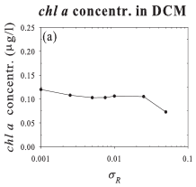
Figure 12: Magnitude, depth, and width of the DCM as a function of $\sigma_{R}$ obtained from the model for site L1129b (panels a, b, c) and site L1105 (panels d, e, f).

A quantitative comparison of each theoretical chl a distribution (red line) with the corresponding experimental one (green line) was carried out by performing $\chi^{2}$ goodness-of-fit test. The results are shown in Tables 2, where $\tilde{\chi}^{2}$ indicates the reduced chi-square. Results of the $\chi^{2}$ test show that the smallest difference between theoretical and experimental chl a distributions is obtained for $\sigma_{b}=0.22$ in site L1129b and $\sigma_{b}=0.15$ in site L1105. We also note that the depths of the DCMs are almost the same as in the deterministic case.
In order to better analyze this aspect, we study for both sites the behaviour of the magnitude, depth, and width of the DCM as a function of $\sigma_{b}$. The results, shown in Fig. 9, indicate that the depth of the DCM is almost constant for $\sigma_{b}\leq 0.4$, increasing for higher values of the noise intensity (see panels b, e of Fig. 9). Conversely, the width of DCM is characterized by a non-monotonic behaviour for increasing noise intensities. In particular, we note that the width of the DCM exhibits a maximum in both sites (for $\sigma_{b}\leq 0.4$ in site L1129b and $\sigma_{b}\leq 0.3$ in site L1105). For higher noise intensities the width tends to zero for site L1129b, while a minimum is present for site L1105 at $\sigma_{b}\leq 0.5$. However, for $\sigma_{b}>0.4$, the values of the DCM width are less significant, since the chl a concentration along the water column and in particular in the DCM decrease strongly, as can be checked in panels a, d. In particular, random fluctuations, cause the reduction of biomass concentration and its displacement along the water column, determining the extinction of the picophytoplankton in the presence of higher intensities of noise. In this condition a clear determination of the DCM becomes more difficult. As a consequence, the values of depth and width for the DCM are less reliable. This analysis shows that the stationary conditions of the system depends strongly on the environmental fluctuations, which play a critical role in determining the best life conditions for the picophytoplankton species.
We complete the analysis of the stochastic dynamics, considering the noise source which affects directly the nutrient concentration (case 2). By numerically solving the corresponding equations of motion (see Eqs. (4),(5),(7),(8),(10)) and averaging over $1000$ realizations, we obtain the average chl a distributions shown in Figs. 10 and 11. The results show that also for low noise intensities ($\sigma_{R}$ between $0.001$ and $0.005$), a decrease and a deeper localization of the DCMs are present. The shape of the chl a peaks exhibits, for both sites, a better agreement with the corresponding experimental DCMs respect to the deterministic case. In particular, for site L1129b the best value of the $\chi^{2}$ test is obtained for $\sigma_{R}=0.0020$, while for site L1105 the best fitting results for $\sigma_{R}=0.0015$ (see Table 3). We note that in site L1129b the best agreement between experimental and numerical distributions is obtained, both in case 1 and case 2, for values of the noise intensity, $\sigma_{b}$ and $\sigma_{R}$, higher than those of site L1105. This can be explained by the fact that in site L1129b the DCM is localized at a depth shallower than in site L1105 (88m vs. 111 m), causing the environmental variables to be subject to more intense random fluctuations due to the closer sea surface. As a consequence, the chl a peak in site L1129b ($88$ m) is more strongly affected by the environmental noise than in site L1105 ($111$ m). The results, shown in Fig. 12, indicate that the depth of the DCM slightly increases in both sites as a function of the noise intensity (see panels b, e of Fig. 12). We note also that a decrease of the chl a concentration is observed in the DCMs of the two sites. This decrease is more rapid in site L1105 (panel d), where a chl a concentration $\sim 0.025$ is reached for $\sigma_{R}\sim 0.01$. Analogously we observe an increase, faster in site L1105, of the width of the DCM. The spread of DCM and reduction of its magnitude are strictly connected with each other. In fact, the decrease of chl a concentration determines a flattening of the DCM with a consequent increase of its width. In conclusion the results shown in Fig. 12 indicate that the phytoplankton biomass tends to disappear for $\sigma_{R}\sim 0.01$, a value lower than those used in case 1, where no extinction occurs up to $\sigma_{b}\sim 0.7$ (see panels a, d of Fig. 9). This indicates that the stability of the nutrient concentration is a critical factor in the dynamics of the ecosystem. Indeed, random fluctuations of the nutrient concentration can produce dramatic effects such as the collapse of phytoplankton biomass considered in our model.
The previous analysis indicates that our model is able to reproduce the phytoplankton distributions observed in real data, without the model taking into account explicitly the environmental variables such as salinity and temperature. However, we observe that, in case 2, the spatio-temporal dynamics of nutrients has been modeled by introducing noise sources which can be interpreted as the effect of random fluctuations of environmental variables, among which salinity and temperature.

V Discussion and Conclusions

In this work we presented a stochastic model, devised starting from previous deterministic models (Litchmann and Klausmeier, 2001; Huisman et al., 2006), to study the spatio-temporal dynamics of the phytoplankton biomass along water column in two different sites of Sicily Channel. In our study, for fixed v, we chose values of the vertical turbulent diffusivity $D_{b}$ which determine the absence of intrinsic oscillations of the phytoplankton concentration, maintaining the system far from the chaos. In oligotrophic waters, typical of Mediterranean Sea, where the surface mixed layer is depleted of nutrients, subsurface maxima of chlorophyll concentration and phytoplankton biomass are often found. Such deep chlorophyll maxima are permanent features in large parts of the tropical and subtropical oceans (Venrick et al., 1973; Cullen, 1982; Mann and Lazier, 1996; Longhurst, 1998; Letelier et al., 2004). Furthermore, seasonal DCMs commonly develop in temperate regions (Venrick, 1993; Longhurst, 1998) and even in the polar oceans (Holm-Hansen and Hewes, 2004), when nutrients are depleted in the surface layer with the onset of the summer season. Here we extend recent phytoplankton models (Klausmeier and Litchman, 2001; Huisman et al., 2002; Fennel and Boss, 2003; Hodges and Rudnick, 2004; Huisman et al., 2004) to show that the phytoplankton distributions, due to random changes, can exhibit fluctuations.
Our work consists in the analysis and subsequent modelling, based on stochastic equations, of data from Sicily Channel, where the waters are prevalently oligotrophic, the climatic conditions are those typical of a temperate region, and the DCMs show stable features for given conditions of light and food resources. For values of depth ranging from $60$ to $110$ meters the presence of a deep chlorophyll maximum indicates the existence of favourable life conditions for the phytoplankton and results in a good agreement with other experimental works, where higher biomass concentration and greater diversity are observed between $60$ and $90$ meters. At the depths considered in this work the light intensity is strongly reduced respect to the surface value (1% of the surface irradiance at 75 m). However, the low light intensity did not appear to limit the diversification of the phytoplankton community (Brunet et al., 2008; Dimier et al., 2009a). In fact, at depths ranging from $60$ to $90$ meters a greater bio-diversity is observed. This can be explained considering that, at these values of depth, the high concentration of nutrients determines the most favourable life conditions for many species of phytoplankton (Reynolds, 1998). Differences in the composition of phytoplankton between the surface and the DCMs are evident mainly for the smaller size class (less than $3$ $\mu m$), which exhibits greater bio-diversity at depths between $60$ and $90$ meters. This could be due to the fact that different species of phytoplankton exhibit different responses to the limiting conditions. We recall that in the marine sites analyzed in this work the incident light intensity is characterized by high values ($I_{in}>1300$ $\mu mol$ photon $m^{-2}s^{-1}$). Therefore, close to the surface the low nutrient concentration represents a limiting condition for all the phytoplankton species, so that the biomass concentration increases with depth. However, for larger values of depth the light intensity becomes a main limiting factor for some species, such as Synechococcus, which show a low degree of adaptability to smaller values of light intensity (Moore et al., 1995; Brunet et al., 2008). This causes Prochlorococcus and picoeukaryotes, which show a high degree of genetic plasticity  (Bibby et al., 2003) and tolerate lower light intensities (Moore et al., 1995, 1998; Dimier et al., 2007), to exhibit a dominance in the deep chlorophyll maximum (Brunet et al., 2007).
In our model, the values of the biological parameters are those of the picoeukaryotes and the environmental parameters are set at values typical of the oligotrophic waters during the warm period. These values allow to obtain chl a distributions along the water column in a good agreement with the experimental data and provide limiting conditions typical of the south part of Mediterranean Sea during the summer. Changes in the phytoplankton composition, both qualitatively and quantitatively, are related to the different depths considered, with light intensity and nutrient availability being the most important factors. Picophytoplankton demonstrated greater ability for photoacclimation than nano- and micro-phytoplankton (Brunet et al., 2003, 2006, 2007; Dimier et al., 2007; Brunet et al., 2008; Dimier et al., 2009a). In fact, a higher contribution of picoeukaryotes to the phytoplankton biomass is observed, specifically pelagophytes and prymnesiophytes, which were also found to thrive elsewhere in cyclonic eddies (Olaizola et al., 1993; Vaillancourt et al., 2003). This ability was also observed in culture (Dimier et al., 2007, 2009a, 2009b).
On the basis of our theoretical findings we can conclude that the position of the deep chlorophyll maximum depends on the parameter values used in the model. We used values of the buoyancy velocity v and vertical turbulent diffusivity $D_{b}$, for which no oscillations occur. In this work we used the condition $D_{b}=D_{R}=0.5\thinspace cm^{2}/s$, corresponding to poorly mixed waters along the whole water column, which causes the phytoplankton peak to have a width of few meters, as observed in the experimental data. Moreover, we also considered in our model the presence of an upper mixed layer, above the thermocline, characterized by a higher value of the diffusion coefficients ($D_{b}=D_{R}=50\thinspace cm^{2}/s$), keeping $D_{b}=D_{R}=0.5$ $cm^{2}/s$ for greater depth (Ryabov et al., 2010). The results (here not shown) did not evidence any variations in the picophytoplankton distributions respect to the case of uniform diffusion coefficients ($D_{b}=D_{R}=0.5$ $cm^{2}/s$) along the whole water column. This can be explained noting that in the ecosystem considered here the mixed layer, due to the depth of the thermocline, is not enough thick to influence the DCMs of the chlorophyll distributions.
In our ecosystem the position and stability of the chlorophyll maximum, obtained from the model, depend not only on the vertical turbulent diffusivity, but also on the nutrient concentration at the bottom $R_{in}$ and the maximum specific growth rate $r$. We also note that the values of $R_{in}$ used in our model are compatible with the nutrient concentrations measured along the water column in several sites of the Mediterranean Sea (Ribera d’Alcalà et al., 2003; Brunet et al., 2006, 2007).
Our numerical results were calculated by setting the maximum specific growth rate $r$ at a value consistent with experimental observations. Specifically, this value has been chosen so that the net per capita growth rate $g(z,t)$, used in the model, is in a good agreement with those experimentally observed for the picoeukaryotes (Jacquet et al., 2001; Timmermans et al., 2005; Dimier et al., 2009b).
We recall that the estimations of the chl a content per picoeukaryote cell are highly variable, depending on the depth and water properties (oligotrophic or eutrophic) examined. Moreover these estimations reflect the taxonomic, ecological and physiological diversity and the plasticity highlighted in previous studies  (Moon-Van Der Staay et al., 2000, 2001; Not et al., 2005; Timmermans et al., 2005). In our model we took into account this aspect. In particular, after obtaining the numerical results for the phytoplankton concentration expressed in number of cells/$m^{3}$, we used the experimental findings given in Ref. (Brunet et al., 2007) to convert the numerical results into chl a concentration expressed in $\mu g/l$. Specifically, because of the peculiarities of our model, suitable to describe the dynamics of the picoeucaryotes, we used the conversion curves typical of these species and compared the results with the experimental chl a concentrations sampled in two different sites of the Mediterranean Sea (Channel of Sicily). From the comparison we found that the values of chl a concentration obtained numerically are in a good agreement not only with our data but also with those measured by Brunet et al. (Brunet et al., 2007). In addition, we note that our numerical results for the picoeukaryote concentration expressed in number of cells/$m^{3}$ match the corresponding experimental data reported in Refs. (Brunet et al., 2006, 2007).
More precisely, as a first step we used a deterministic model, consisting of an auxiliary equation for the light intensity and two differential equations, one for the dynamics of the phytoplankton biomass, the other for the dynamics of the nutrients. The numerical results showed a good qualitative agreement with the real data, even if discrepancies were observed between the characteristics of the chl a concentration profiles provided by the model and those obtained from the real data.
To improve the agreement between numerical and experimental distributions, we modeled the random fluctuations of the environmental variables, by adding a term of multiplicative Gaussian noise in the differential equation for the phytoplankton biomass. The results obtained indicate that the presence of random fluctuations, acting directly on the phytoplankton biomass, determines chl a stationary distributions more similar to the experimental ones. In particular, we found that both the position and magnitude of the DCMs agree very well with the experimental findings. Afterwards, we modified the deterministic model considering the role of a noise source which influences directly the dynamics of the nutrients, by adding a term of multiplicative Gaussian noise in the differential equation for the nutrients. In this case we observed for suitable noise intensities (much lower than those used in the equation for the phytoplankton biomass) a further improvement of the numerical distributions of chl a concentration respect to the experimental ones. In addition, we found that higher noise intensities (comparable with those used in the equation for the phytoplankton biomass), cause a rapid extinction of the phytoplankton community. The results obtained indicate that the proposed stochastic model is able to reproduce patterns of real phytoplankton distributions when aquatic ecosystems with poorly mixed waters are considered.

References

- Spagnolo et al. (2004) B. Spagnolo, D. Valenti, and A. Fiasconaro, Math. Biosci. Eng. 1, 185 (2004).
- Huppert et al. (2005) A. Huppert, B. Blasius, R. Olinkya, and L. Stone, J. Theor. Biol. 236, 276 (2005).
- Ebeling and Spagnolo (2005) W. Ebeling and B. Spagnolo, Fluct. Noise Lett. 5, L159 (2005).
- Provata et al. (2008) A. Provata, I. Sokolov, and B. Spagnolo, Eur. Phys. J. B 65, 307 (2008).
- Spagnolo and Dubkov (2008) B. Spagnolo and A. A. Dubkov, Int. J. Bifurcat. Chaos 18, 2643 (2008).
- Valenti et al. (2008) D. Valenti, L. Tranchina, C. Cosentino, M. Brai, A. Caruso, and B. Spagnolo, Ecol. Model. 213, 449 (2008).
- Grenfell et al. (1998) B. T. Grenfell, K. Wilson, B. F. Finkenstädt, T. N. Coulson, S. Murray, S. D. Albon, J. M. Pemberton, T. H. Clutton-Brock, and M. J. Crawley, Nature 394, 674 (1998).
- Zimmer (1999) C. Zimmer, Science 284, 83 (1999).
- Bjørnstad and Grenfell (2001) O. N. Bjørnstad and B. T. Grenfell, Science 293, 638 (2001).
- Spagnolo et al. (2002) B. Spagnolo, M. Cirone, A. L. Barbera, and F. de Pasquale, J. Phys. 14, 2247 (2002).
- La Barbera and Spagnolo (2002) A. La Barbera and B. Spagnolo, Physica A 314, 120 (2002).
- Spagnolo and La Barbera (2002) B. Spagnolo and A. La Barbera, Physica A 315, 114 (2002).
- Spagnolo et al. (2003) B. Spagnolo, A. Fiasconaro, and D. Valenti, Fluct. Noise Lett. 3, L177 (2003).
- Spagnolo et al. (2005) B. Spagnolo, D. Valenti, and A. Fiasconaro, Prog. Theor. Phys. Supp. 157, 312 (2005).
- Caruso et al. (2005) A. Caruso, M. E. Gargano, D. Valenti, A. Fiasconaro, and B. Spagnolo, Fluct. Noise Lett. 5, L349 (2005).
- Chichigina et al. (2005) O. Chichigina, D. Valenti, and B. Spagnolo, Fluct. Noise Lett. 5, L243 (2005).
- Fiasconaro et al. (2006) A. Fiasconaro, D. Valenti, and B. Spagnolo, Eur. Phys. J. B 50, 189 (2006).
- Valenti et al. (2006) D. Valenti, L. Schimansky-Geier, X. Sailer, and B. Spagnolo, Eur. Phys. J. B 50, 199 (2006).
- Chichigina (2008) O. A. Chichigina, Eur. Phys. J. B 65, 347 (2008).
- Klausmeier and Litchman (2001) C. A. Klausmeier and E. Litchman, Limnol. Oceanogr. 46, 1998 (2001).
- Klausmeier et al. (2007) C. A. Klausmeier, E. Litchman, and S. A. Levin, J. Theor. Biol. 246, 278 (2007).
- Anderson (1969) G. C. Anderson, Limnol. Oceanogr. 14, 386 (1969).
- Cullen (1982) J. J. Cullen, Can. J. Fish. Aquat. Sci. 39, 791 (1982).
- Abbott et al. (1984) M. R. Abbott, K. L. Denman, T. M. Powell, P. J. Richerson, R. C. Richards, and C. R. Goldman, Limnol. Oceanogr. 29, 862 (1984).
- Tittel et al. (2003) J. Tittel, V. Bissinger, B. Zippel, U. Gaedke, E. B. A. Lorke, and N. Kamjunke, P. Natl. Acad. Sci. USA 100, 12776 (2003).
- Radach and Maier-Reimer (1975) G. Radach and E. Maier-Reimer, Mem. Soc. Roy. Sci. de Liege 6e serie, 113 (1975).
- Varela et al. (1992) R. A. Varela, A. Cruzado, J. Tintore, and E. G. Ladona, J. Mar. Res. 50, 441 (1992).
- Huisman and Weissing (1995) J. Huisman and F. J. Weissing, Am. Nat. 146, 536 (1995).
- Diehl (2002) S. Diehl, Ecology 83, 386 (2002).
- Hodges and Rudnick (2004) B. A. Hodges and D. L. Rudnick, Deep-Sea Res. Pt. I 51, 999 (2004).
- Beckmann and Hense (2007) A. Beckmann and I. Hense, Prog. Oceanogr. 75, 771 (2007).
- Mei et al. (2009) Z. P. Mei, Z. V. Finkel, and A. J. Irwin, J. Theor. Bio. 259, 582 (2009).
- Bougaran et al. (2010) G. Bougaran, O. Bernard, and A. Sciandra, J. Theor. Biol. 265, 443 454 (2010).
- Venrick (1993) E. L. Venrick, Limnol. Oceanogr. 38, 1135 (1993).
- Holm-Hansen and Hewes (2004) O. Holm-Hansen and C. D. Hewes, Polar Biol. 27, 699 (2004).
- Ryabov et al. (2010) A. B. Ryabov, L. Rudolf, and B. Blasius, J. Theor. Biol. 263, 120 (2010).
- Norberg (2004) J. Norberg, Limnol. Oceanogr. 49, 1269 (2004).
- Fogg (1991) G. E. Fogg, New Phytol. 118, 191 (1991).
- Prézelin et al. (1991) B. B. Prézelin, M. M. Tilzer, O. Schofield, and C. Haese, Aquat. Sci. 53, 136 (1991).
- Barale et al. (2008) V. Barale, J. M. Jaquet, and M. Ndiaye, Remote Sens. Environ. 112, 3300 (2008).
- Lermusiaux and Robinson (2001) P. F. J. Lermusiaux and A. R. Robinson, Deep-Sea Research I 48, 1953 (2001).
- Lafuente et al. (2002) J. G. Lafuente, A. Garcia, S. Mazzola, L. Quintanilla, J. Delgado, A. Cuttita, and B. Patti, Fish Oceanogr. 11, 31 (2002).
- Cuttitta et al. (2003) A. Cuttitta, V. Carini, B. Patti, A. Bonanno, G. Basilone, S. Mazzola, J. García Lafuente, and A. García, Hydrobiologia 503, 117 (2003).
- Basilone et al. (2004) G. Basilone, C. Guisande, B. Patti, S. Mazzola, A. Cuttitta, A. Bonanno, and A. Kallianiotis, Fish. Res. 68, 9 (2004).
- Brankart (1994) J. M. Brankart, Technical Report, University of Liege (1994).
- Olson et al. (1993) R. J. Olson, E. R. Zettler, and M. D. DuRand, Phytoplankton analysis using flow cytometry (pgs. 175-186). In: Handbook of methods in aquatic microbial ecology (Lewis Publishers, Boca Raton, FL, USA, 1993).
- Brunet et al. (2008) C. Brunet, R. Casotti, and V. Vantrepotte, J. Plankton Res. 30, 645 (2008).
- Brunet et al. (2006) C. Brunet, R. Casotti, V. Vantrepotte, F. Corato, and F. Conversano, Aquat. Microb. Ecol. 44, 127 (2006).
- Brunet et al. (2007) C. Brunet, R. Casotti, V. Vantrepotte, and F. Conversano, Mar. Ecol. Prog. Ser. 346, 15 (2007).
- Dimier et al. (2007) C. Dimier, F. Corato, G. Saviello, and C. Brunet, J. Phycol. 43, 275 283 (2007).
- Dimier et al. (2009a) C. Dimier, G. Saviello, F. Tramontano, and C. Brunet, Protist 160, 397 (2009a).
- Raven et al. (2005) J. A. Raven, Z. V. Finkel, and A. J. Irwin, J. Geophys. Res. 55, 209 (2005).
- Worden and Not (2008) A. Z. Worden and F. Not, Microbial Ecology of the Oceans, Second Edition (John Wiley & Sons, Inc., 2008).
- Raven (1998) J. A. Raven, Funct. Ecol. 12, 503 (1998).
- Brunet et al. (2003) C. Brunet, R. Casotti, B. Aronne, and V. Vantrepotte, J. Plankton Res. 25, 1413 (2003).
- Finkel and Irwin (2005) Z. V. Finkel and A. J. Irwin, Vie Milieu 55, 209 (2005).
- Casotti et al. (2003) R. Casotti, A. Landolfi, C. Brunet, F. D’Ortenzio, O. Mangoni, and M. Ribera d’Alcalà, J. Geophys. Res. 108 (2003).
- Turpin (1988) D. H. Turpin, Physiological mechanisms in phytoplankton resource competition (316-368). In: Growth and reproductive strategies of freshwater phytoplankton (Cambridge University Press, 1988).
- Huisman et al. (2006) J. Huisman, N. P. T. Thi, D. M. Karl, and B. Sommeijer, Nature 439, 322 (2006).
- Shigesada and Okubo (1981) N. Shigesada and A. Okubo, J. Math. Biol. 12, 311 (1981).
- Kirk (1994) J. T. O. Kirk, Light and Photosynthesis in Aquatic Ecosystems ( edition) (Cambridge University Press, 1994).
- Dimier et al. (2009b) C. Dimier, C. Brunet, R. Geider, and J. Raven, Limnol. Oceanogr. 54, 823 (2009b).
- Giuffrida et al. (2009) A. Giuffrida, D. Valenti, G. Ziino, B. Spagnolo, and A. Panebianco, Eur. Food Res. Technol. 228, 767 (2009).
- Litchmann and Klausmeier (2001) E. Litchmann and C. A. Klausmeier, Am. Nat. 157, 170 (2001).
- Venrick et al. (1973) E. L. Venrick, J. A. McGowan, and A. W. Mantyla, Fish. Bull. 71, 41 (1973).
- Mann and Lazier (1996) K. H. Mann and J. R. N. Lazier, Dynamics of marine ecosystems (Blackwell Publishing, Malden, MA, USA, 1996).
- Longhurst (1998) A. R. Longhurst, Ecological geography of the sea (Academic Press, San Diego, California, USA, 1998).
- Letelier et al. (2004) R. M. Letelier, D. M. Karl, M. R. Abbott, and R. R. Bidigare, Limnol. Oceanogr. 49, 508 (2004).
- Huisman et al. (2002) J. Huisman, M. Arrayas, U. Ebert, and B. Sommeijer, Am. Nat. 159, 245 (2002).
- Fennel and Boss (2003) K. Fennel and E. Boss, Limnol. Oceanogr. 48, 1521 (2003).
- Huisman et al. (2004) J. Huisman, J. Sharples, J. M. Stroom, P. M. Visser, W. E. N. Kardinaal, J. M. H. Verspagen, and B. Sommeijer, Ecology 85, 2960 (2004).
- Reynolds (1998) C. S. Reynolds, Verh. Internat. Verein. Limnol. 23, 683 (1998).
- Moore et al. (1995) L. R. Moore, R. Goericke, and S. W. Chisholm, Mar. Ecol. Prog. Ser. 116, 259 (1995).
- Bibby et al. (2003) T. S. Bibby, I. Mary, J. Nield, F. Partensky, and J. Barber, Nature 424, 1051 (2003).
- Moore et al. (1998) L. R. Moore, G. Rocap, and S. W. Chisholm, Nature 397, 464 (1998).
- Olaizola et al. (1993) M. Olaizola, D. A. Ziemann, P. K. Bienfang, W. A. Walsh, and L. D. Conquest, Mar. Biol. 116, 533 (1993).
- Vaillancourt et al. (2003) R. D. Vaillancourt, J. Marra, M. P. Seki, M. L. Parsons, and R. R. Bidigare, Deep Sea Res. II 50, 829 (2003).
- Ribera d’Alcalà et al. (2003) M. Ribera d’Alcalà, G. Civitarese, F. Conversano, and R. Lavezza, J. Geophys. Res. 108 (2003).
- Jacquet et al. (2001) S. Jacquet, F. Partensky, J. F. Lennon, and D. Vaulot, J. Phycol. 37, 357 (2001).
- Timmermans et al. (2005) K. R. Timmermans, B. Van Der Wagt, M. J. W. Veldhuis, A. Maathan, and H. J. W. De Baar, J. Sea Res. 53, 109 (2005).
- Moon-Van Der Staay et al. (2000) S. Y. Moon-Van Der Staay, G. W. M. Van Der Staay, L. Guillou, and D. Vaulot, Limmol. Oceanogr. 45, 98 (2000).
- Moon-Van Der Staay et al. (2001) S. Y. Moon-Van Der Staay, R. De Wachter, and D. Vaulot, Nature 409, 607 (2001).
- Not et al. (2005) F. Not, R. Massana, M. Latasa, D. Marie, C. Colson, W. Eikrem, C. Pedròs-Aliò, D. Vaulot, and N. Simon, Limnol. Oceanogr. 50, 1677 1686 (2005).