Local Potential Model of the Hoyle Band in ¹²C

Abstract

We describe the excited $0^{+}$ state of ¹²C at 7.654 MeV, often called the Hoyle state, in terms of a local potential ⁸Be+$\alpha$ cluster model. We use a previously published prescription for the cluster-core potential to solve the Schrödinger equation to obtain wave functions for this state, and also for higher angular momentum states of the same system. We calculate energies, widths and charge radii for the resulting band of states, with particular emphasis on the recently discovered $2^{+}$ state. We examine various choices of the global quantum number $G=2n+L$ for the cluster-core relative motion, and find that $G=6$ leads to the most coherent description of the properties of the states and is consistent with recent experimental data on the $L=2$ state.

I Introduction

When considering how carbon could be produced in stellar nucleosynthesis, Hoyle [Hoyle_1] famously predicted that the ¹²C nucleus must have an excited $0^{+}$ state in the vicinity of the 3-$\alpha$ breakup threshold. Such a state was duly found [Dunbar] in short order on the basis of Hoyle’s suggestion. Its existence was essential for ¹²C to be produced at an adequate rate to open up the pathways to the synthesis of still heavier nuclei [Hoyle_2] . Not only had this state escaped both experimental detection and theoretical prediction up to that point, but it has continued to pose severe challenges to nuclear structure models ever since.

The shell model struggles to describe any low-lying excited $0^{+}$ states in p-shell and sd-shell nuclei. To this day, the most advanced no-core shell model has not succeeded in reproducing the excitation energy of the Hoyle state [Navratil] . Models invoking a 3$\alpha$ chain [Morinaga] ; [Horiuchi_1] ; [Me_Rae] were able to accommodate the excitation energy, but could not reproduce the decay width of the Hoyle state. Better success was enjoyed by orthogonality condition model calculations of the 3$\alpha$ system, using a semi-microscopic $\alpha-\alpha$ interaction [Horiuchi_2] ; [Saito] , which gave a suitably sized $\alpha$-decay width in the ⁸Be$(0_{1}^{+})+\alpha$ channel. This suggested that the dominant structure of the Hoyle state must be ⁸Be$(0_{1}^{+})+\alpha$ in a relative s-state. Such a conclusion was backed up by fully microscopic $3\alpha$ calculations using the Resonating Group and Generator Coordinate Methods [Hack] ; [Kamimura] ; [Uegaki] ; [Descouv] . More recently fully microscopic calculations using Antisymmetrized Molecular Dynamics (AMD) [Enyo] and Fermionic Molecular dynamics (FMD) [Feld] have been able to give a good account of the low-lying spectrum of ¹²C without assuming alpha clustering a priori. For the particular case of the very loosely bound Hoyle state a three-$\alpha$ condensate wave function [FunakiCondensate] has also been shown to have a large overlap with the FMD wave function. The current situation is well summarized in a recent review [HIK] .

In parallel with these theoretical developments, new life has recently been breathed into the experimental program. Given that the Hoyle state has a large mean square radius, it is natural to suggest calculating higher angular momentum states with this same structure thereby producing a band of excited states with a large moment of inertia. Although Friedrich et al. [Friedrich] claim there are no such rotational states, most $3\alpha$ models do support them, with the $2^{+}$ state generally expected to have an excitation energy in the region of 10 MeV. Initial searches for this $2^{+}$ state via beta decay [Fynbo] were discouraging, but in recent times three separate experiments have provided evidence of its existence. Itoh et al. [Itoh] see a $2^{+}$ state at 9.9 MeV, with a width of 1.0 MeV, via inelastic $\alpha$-particle scattering in their ¹²C($\alpha,\alpha^{\prime}$) measurements. Freer et al. [Freer] see a $2^{+}$ state at 9.6 MeV, with a width of 0.6 MeV, in their inelastic proton scattering ¹²C(p,p^′) work. Gai [Gai] confirms the existence of a $2^{+}$ state around 10 MeV (but without being able to measure a width) in photonuclear disintegration ¹²C($\gamma,3\alpha$) studies.

In view of this resurgent interest in an excited Hoyle band we ask in this paper to what extent the known data can be accounted for (and further excited states predicted) by a local potential ⁸Be+$\alpha$ cluster model. This model provides a physically transparent and calculationally straightforward description of the energies, widths and charge radii of the known states in the proposed Hoyle band. It also throws some light on the question of how high in angular momentum such a band might continue. In this way it can be a useful guide to experimental groups searching for as yet unidentified higher $L$ states. It is also illuminating to see how far one can get with a simple but physically motivated model. Although ideally the full rigours of a more microscopic and computationally intensive approach might seem preferable, a rather simplified effective nucleon-nucleon potential is needed to carry this to fruition. It might be that a phenomenological approach can produce a band of states with properties closer to the experimental values. In any event it is interesting to compare the results from different theoretical treatments with each other as well as with experiment.

In the next section we describe our local potential ⁸Be+$\alpha$ cluster model. After that, we compare the model’s results with the available data and discuss the possible existence of additional states. Finally, we summarize our conclusions.

II Local potential cluster model

The cluster model employed here was first proposed to study the excited 4p-4h band of ¹⁶O (bandhead at 6.05 MeV) and the ground state band of ²⁰Ne [BDV] and has subsequently been applied to a wide range of nuclei across the Periodic Table from ⁶Li to ²⁴²Cm. However, it has not previously been used for ¹²C, because the ground state band of that nucleus is known to be oblate (from the sign of its quadrupole moment [Vermeer] ) and a two-body cluster-core system inevitably produces a prolate deformation. This is because, for spinless constituents like ⁸Be and $\alpha$, the quadrupole operator for the system reduces to

$$M(E2)={(Z_{1}A_{2}^{2}+Z_{2}A_{1}^{2})\over(A_{1}+A_{2})^{2}}R^{2}Y_{2}(\hat{\bf R})$$ (1)

The expectation value of this operator always yields a positive quadrupole moment, indicating a prolate spheroidal shape. To obtain negative quadrupole moments, appropriate to oblate shapes, it is necessary to consider three-body systems. This outcome provides a large part of the motivation behind attempts to model the ground state band of ¹²C (and indeed the excited $3^{-}$ state at 9.64 MeV) as an equilateral triangular arrangement of three $\alpha$ particles [HafstadTeller] . However, the indications that the Hoyle state, and any associated rotations of it, have a large ⁸Be$(0_{1}^{+})+\alpha$ component, mark out the Hoyle band as ideal territory for our local potential two-body cluster model. Unfortunately, this does mean that we are unable to address any states of the ¹²C system that do not have this particular structure. In particular, we cannot model the ground state band and the excited $3^{-}$ state mentioned above.

In general, we model a nucleus as two even-even sub-nuclei of mass $A_{1}$ and $A_{2}$ separated by a distance ${\bf R}$, interacting through a deep, local nuclear potential $V_{N}(R)$ and a Coulomb potential $V_{C}(R)$ appropriate to a point cluster and a uniformly charged spherical core. The nuclear part has previously been parametrised in the form [univ] :

$$V_{N}(R) = -V_{0}\Biggl{\{}{x\over[1+\exp{((R-R_{0})/a))}]}$$

$$+ {1-x\over[1+\exp{((R-R_{0})/3a)}]^{3}}\Biggr{\}}$$ (2)

with parameter values given by

$$v_{0}=54.0\ {\rm MeV,}\ \ \ a=0.73\ {\rm fm,}\ \ \ {\rm and}\ \ \ x=0.33$$ (3)

and $V_{0}$ related to $v_{0}$ by

$$V_{0}={\displaystyle{A_{1}A_{2}\over(A_{1}+A_{2}-1)}v_{0}\over{\displaystyle{x\over[1+\exp{(-R_{0}/a)}]}+{1-x\over[1+\exp{(-R_{0}/3a)}]^{3}}}}.$$ (4)

The radius parameter $R_{0}$ of the potential is determined by fitting to the experimental energy of the spectrum’s band head, and is linked to the choice of $G=2n+L$ (see below). This potential is now incorporated into the cluster-core relative motion Hamiltonian $H_{0}({\bf R})$, and the resulting Schrödinger equation

$$H_{0}({\bf R})\Phi_{GnL}({\bf R}) = E_{GnL}\Phi_{GnL}({\bf R})$$

$$= E_{GnL}{u_{GnL}(R)\over R}Y_{LM}(\theta,\phi).$$ (5)

is solved numerically. We label the wave functions and energies with the global quantum number $G=2n+L$, where $n$ is the number of internal nodes in the radial wave function and $L$ the orbital angular momentum.

We must choose the value of $G$ large enough to guarantee that the Pauli exclusion principle is satisfied by excluding the cluster constituents from states occupied by the core nucleons. For the ⁸Be + $\alpha$ system this requires $G\geq 4$. The appropriate choice of $G$ is not clear cut when we are not using an oscillator potential, although we can certainly use oscillator considerations as a guide. The lowest allowed value, $G=4$, would correspond to packing the $\alpha$ nucleons into the p-shell, which seems an unlikely description of an excited state in ¹²C. Nevertheless, for completeness, we present calculations employing $G=4,6$ and 8, with a view to deciding a posteriori on the basis of a comparison with experimental data which is the best choice. Indeed, only a posteriori can we say that our model, with any eventually preferred value of $G$, is appropriate for describing the Hoyle state and its associated band by comparing its predictions with the measured properties of those states.

Although numerical solution of the Schrödinger equation without any restrictions on $G$ certainly does produce lower lying states, they are Pauli forbidden and do not correspond to physical states of ¹²C. Thus, we have no ¹²C bound states in our model and cannot use it to describe the observed ground $0^{+}$ or excited $2^{+}$ (4.44 MeV) states of the nucleus. Equally, we cannot describe the $3^{-}$ (9.64 MeV) state of ¹²C (as explained earlier). It is possible to produce negative parity states in our model by solving the Schrödinger equation with an odd value of $G$, but the resulting energies are 10–20 MeV above the Hoyle state, and not of immediate interest. Similarly, we could obtain negative parity states of ¹²C by using even $G$ values in conjunction with an excited negative parity state of the ⁸Be core. Again, the resulting excitation energies in ¹²C are too high to be of interest in the current study.

As a further model extension we could include excitations of the ⁸Be core into its $2^{+}$ and $4^{+}$ states. We do not do this here because it would involve the introduction of more adjustable parameters to describe the non-central interactions that accompany such excitations, and we are trying to keep the number of fitted quantities to a minimum. Our previous experience of including core excitations in treatments of ¹⁶O [BBR_O16] and ²⁴Mg [BHM_24Mg] leads us to expect that they would not have a major effect on our conclusions in the the ⁸Be$+\alpha$ case.

Solving the Schrödinger equation produces excitation energies and their associated widths directly. The resulting wave functions can also be used to calculate mean square charge radii of the states from

$$(Z_{1}+Z_{2})\langle R^{2}(^{12}{\rm C})\rangle = Z_{1}\langle R^{2}(^{8}{\rm Be})\rangle+Z_{2}\langle R^{2}(\alpha)\rangle$$

$$+ {(Z_{1}A_{2}^{2}+Z_{2}A_{1}^{2})\over(A_{1}+A_{2})^{2}}\langle R^{2}_{\rm rel}\rangle$$ (6)

where $(Z_{1},A_{1})=(4,8)$ and $(Z_{2},A_{2})=(2,4)$ for the ⁸Be + $\alpha$ system. To apply this formula for charge radii we need to supplement the wave functions generated above with a description of the ground state of ⁸Be (or at least, of its mean square charge radius). An excellent description of $\alpha-\alpha$ scattering phase shifts and ⁸Be has already been given within the local potential cluster model [BFW] using a Gaussian nuclear potential

$$V_{N}(R)=V_{G}\exp{(-\alpha R^{2})}$$ (7)

with $V_{G}=122.6225$ MeV and $\alpha=0.22$ fm^-2 and a Coulomb potential

$$V_{C}(R)={Z_{1}Z_{2}{\rm erf}(\beta R)\over R}$$ (8)

with $\beta=0.75\ {\rm fm}^{-1}$ and where $Z_{1}=Z_{2}=2$ for the $\alpha-\alpha$ system. We adopt this description of ⁸Be wholesale because, within our model, it can hardly be improved upon.

As a consistency check on the widths of the states we can make use of our earlier work (see for example [pdecay] ) on charged particle decay widths. Within the two-body local potential model, a semiclassical approximation leads to an $\alpha$-partial width of

$$\Gamma_{\alpha}=F{\hbar^{2}\over 4\mu}\exp{\left(-2\int_{R_{2}}^{R_{3}}dR\ k(R)\right)},$$ (9)

where $R_{2}$ and $R_{3}$ are the two outermost classical turning points and $\mu$ is the reduced mass of the system. The normalization factor $F$ is given to good accuracy by

$$F\int_{R_{1}}^{R_{2}}{dR\over 2k(R)}=1,$$ (10)

with $R_{1}$ the innermost turning point, and the wave number $k(R)$ is

$$k(R)=\left({2\mu\over\hbar^{2}}|Q-V(R)|\right)^{1/2}$$ (11)

and $Q$ is the experimental energy of the decaying state relative to the two-body breakup threshold.

III Energies, widths and radii of Hoyle band states

As outlined in the previous section, we calculate ⁸Be + $\alpha$ cluster states, using a previously published prescription for the potential [univ] , without adjusting any of the parameters $v_{0}$, $a$ and $x$ listed in Eq.(3). We identify the $0^{+}$ state with the Hoyle state, check that this choice produces a good account of the available data, and proceed to calculate similar states of higher angular momenta. Each band of states is labelled by the choice of $G=2n+L$. The maximum possible value of $L$ in this scheme is equal to $G$ itself (corresponding to the nodeless wave function). We determine the potential radius $R_{0}$ of the potential by fitting so as to reproduce the experimental energy of the $0^{+}$ Hoyle state exactly. The resulting values for $R_{0}$ are listed in Table I. It is also useful to know the position and maximum height of the potential (Coulomb barrier) since this gives an upper limit on the energy of a resonant state with the corresponding value of $L$. Therefore we also list these values in Table I for the three values of $G=4,6$ and 8 under consideration.

Table 1: Potential Maxima for $G=4,6$ and 8

	$V_{\rm max}$ (MeV) at $R_{\rm max}$(fm)
L	$G=4$	$G=6$	$G=8$
	$R_{0}=0.8883$ fm	$R_{0}=1.9386$ fm	$R_{0}=2.9008$ fm
0	1.63 at 6.20	1.42 at 7.25	1.26 at 8.28
2	3.12 at 5.16	2.44 at 6.41	2.02 at 7.56
4	9.23 at 3.48	5.74 at 5.28	4.24 at 6.62
6		13.87 at 4.02	8.82 at 5.74
8			17.26 at 4.86

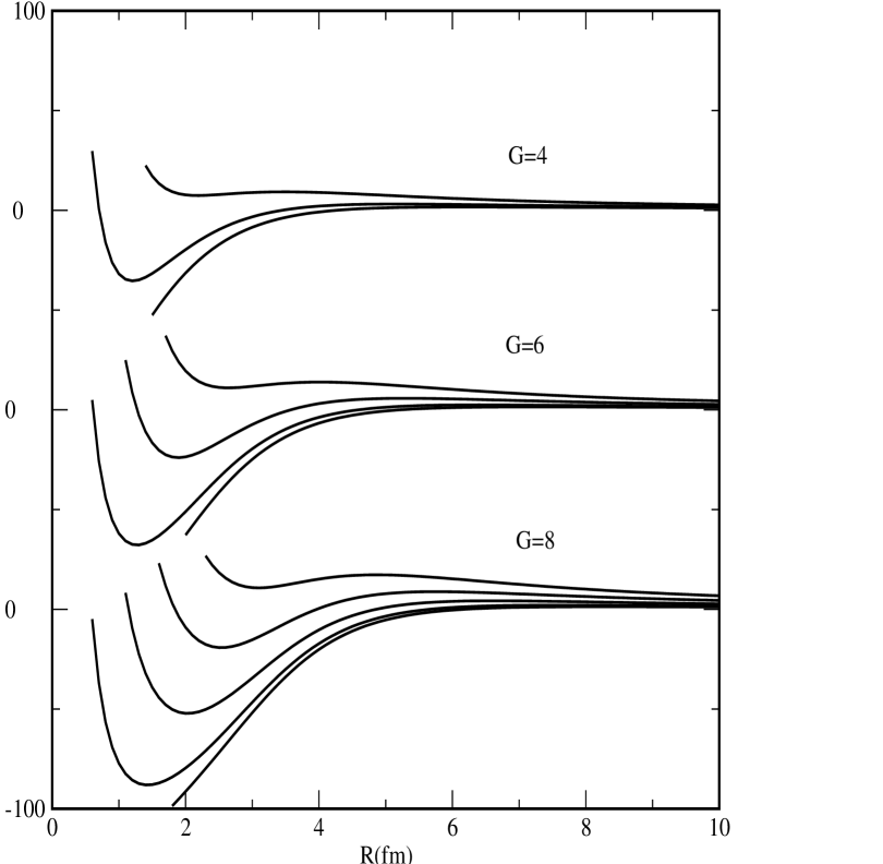
Figure 1: Local potentials (nuclear + Coulomb + centrifugal) for the ⁸Be + $\alpha$ system corresponding to all possible $L$-values for the global quantum numbers $G=4,6$ and 8. The potentials for $G=4$ are displaced upwards by 100 MeV and those for $G=8$ downwards by 100 MeV to aid visibility.

Figure 1 shows the potentials (nuclear, Coulomb and centrifugal combined) obtained from the procedure described above for $G=4,6$ and 8. It is clear from inspection that it would be no surprise to discover that the state with the highest expected $L$-value for each value of $G$ was completely unbound (or at best precariously resonant). In fact, none of the states of the Hoyle band is bound. They are all (at best) resonances, and in some cases rather close to the top of the Coulomb barrier, so the calculation of their energies and widths is numerically delicate. In view of this we have found it expedient to cross check our results using a variety of different calculational methods.

• We use our own bound state code to perform a numerical integration of the Schrödinger equation, but rounding off the potential at its maximum value for radii in excess of that radius where the maximum is achieved (i.e. $V=V_{\rm max}$ for $R\geq R_{\rm max}$). This serves to give a good estimate of the energies which can be used to provide a starting energy for the methods described below, and also as a consistency check on these subsequent results.

• We use the published code GAMOW [Pal] , which employs complex arithmetic to solve the Schrödinger equation and fits Gamow tails to the resonant states, so as to evaluate energies and widths of the states. We need this code principally for the wave functions it generates which can be used eventually in the calculation of the mean square charge radii.

• We use the published elastic scattering code SCAT2 [Bersillon] which allows us to monitor the scattering phase shifts of the ⁸Be + $\alpha$ system as a function of the centre of mass (c.m.) energy, and thereby to identify the peak energies and widths of the resonant states in the various partial waves.

• As an order of magnitude check, we also evaluate the widths of the states using the semiclassical method discussed in the previous section, Eq.(8). Previous experience using this approach to calculate half-lives for charged particle decay suggests that it can be expected to agree with the true value to within about a factor of two.

The code SCAT2 writes out the scattering matrix elements $\eta_{l}$ in the form $1-{\rm Re}(\eta_{l})$ and Im($\eta_{l}$), where the $\eta_{l}$ are related to the transmission coefficients $T_{l}$ by

$$T_{l}=1-|\eta_{l}|^{2}.$$ (12)

We run the code at successively incremented c.m. energies, centred on the values indicated by our own bound state code and by GAMOW, and monitor the behaviour of the scattering matrix as the energy increases through the suspected resonance region. As the energy of a resonant state is approached from below, the value of $1-{\rm Re}(\eta_{l})$ for the appropriate partial wave $l$ rises from near zero through 1 towards 2. We take the energy range over which it rises from 0.5 to 1.5 as the width of the resonant state. The value of Im($\eta_{l}$) also rises from 0 towards 1, and then falls again to zero. By systematically working through the energy regions indicated by the bound state code (and taking successively finer incremental energy grids as necessary), we obtain the width values reported for the $L>0$ states in Table II. The widths for the $0^{+}$ states were obtained using the semiclassical approximation described in the previous section, Eqs.(8-10). We note that the experimental width of the $0^{+}$ state is $8.5\pm 1.0$ eV, with which the corresponding theoretical value obtained with $G=6$ in Table II is in good agreement.

The energies from all these methods are mutually compatible and we present the average of them as the peak energy of each resonance in Table II. We have added 7.365 MeV to the c.m. scattering energies to obtain excitation energies relative to the ¹²C ground state. (Note that the $0^{+}$ state’s energy of 7.654 MeV was used to fit the potential radius $R_{0}$ for all three values of $G$)

Table 2: Calculated state energies, widths and $\langle R^{2}\rangle$ for $G=4,6$ and 8

	$E{\rm(MeV)}\pm\Gamma$
L	$G=4$	$G=6$	$G=8$
0	$7.654\pm 3$(eV)	$7.654\pm 6$(eV)	$7.654\pm 13$(eV)
2	No state	$9.61\pm 360$(keV)	$8.85\pm 68$(keV)
4	No state	$13.71\pm 1.24$(MeV)	$11.52\pm 300$(keV)
6		No state	$16.25\pm 660$(keV)
8			No state
$\langle r^{2}\rangle$	11.688 fm2	13.457 fm2	15.553 fm2
$\sqrt{\langle r^{2}\rangle}$	3.42 fm	3.67 fm	3.94 fm

Figure 2 shows the energy dependence of $1-{\rm Re}(\eta_{l})$ and Im($\eta_{l}$) for the $G=6,L=2$ resonance near the c.m. energy of about 2.22 MeV. This is both a typical case, and the state that we are most interested in (because of recent experimental results [Itoh] ; [Freer] ; [Gai] which have at last found a rotational state of the Hoyle band). The best description of this state within our model is achieved using $G=6$. For $G=4$ there is no resonant state at all, and for $G=8$ the excitation energy is too low and the width too narrow. We are not unduly concerned that this value of $G$ does not tally “nicely” with oscillator shell model considerations, which might suggest G=$8$ since most of the low-lying intruder states in this region are described as 4p-4h excitations in the shell model. We are not using a harmonic oscillator potential and will generate rather different wave functions with exponential rather than Gaussian tails, and so do not expect an identity of $G$ values between the two cases. Our calculations also predict an excited $4^{+}$ state at 13.71 MeV. We predict a width of 1.24 MeV for it, which would make it hard to detect in experiments. We note however that this excitation energy places the state above the barrier maximum for an $L=4$ state in a $G=6$ band, indicating that the result is not completely reliable, although still indicative of a possible $4^{+}$ state in this region.

In this context it is interesting to note that Freer et al.[Freer4] have recently found evidence for a new state in ¹²C at $13.3\pm 0.2$ MeV with a width of $1.7\pm 0.2$ MeV in their studies of the ¹²C(⁴He, ⁴He+⁴He+⁴He) ⁴He and ⁹Be(⁴He, ⁴He+⁴He+⁴He)n reactions. Analysis of the angular distributions suggests that the state might have J${}^{\pi}=4^{+}$. As such, its properties are in line with our expectations for the third state in the Hoyle band, and we await the outcome of further investigations with interest.

Previous analyses of inelastic electron scattering from ¹²C [Funaki] indicate that the Hoyle state has an abnormally large charge radius. We therefore calculate the values of $\langle r^{2}\rangle$ implied by our model for $G=4,6$ and 8. We first need to calculate a mean square charge radius for ⁸Be. We do this by using the mean square charge radius for an $\alpha$-particle of 1.6757 fm [Angeli] and the mean square separation of the two $\alpha$-particles calculated by our bound state code and confirmed by GAMOW using the potential of Ref.[BFW] in the formula

$$\langle R^{2}\rangle_{{}^{8}{\rm Be}}=\langle R^{2}\rangle_{\alpha}+{1\over 4}\langle R^{2}\rangle_{\alpha-\alpha}$$ (13)

This yields a mean square charge radius for ⁸Be of 10.634 fm² (with a square root of 3.261 fm). This, in turn, serves as input for the mean square charge radius of the Hoyle state in the formula

$$\langle R^{2}\rangle_{{}^{12}{\rm C-Hoyle}} = {1\over 3}\langle R^{2}\rangle_{\alpha}+{2\over 3}\langle R^{2}\rangle_{{\rm Be}}$$ (14)

$$+ {2\over 9}\langle R^{2}\rangle_{\alpha-{\rm Be}}$$

Our $G=6$ value of 3.78 fm is somewhat below the value of 3.87 fm deduced by Funaki et al. [Funaki] but significantly larger than the values deduced from earlier GCM calculations of 3.50 fm [Uegaki] and 3.47 fm [Kamimura] obtained from full 3$\alpha$ calculations using Volkov effective two-nucleon forces.

IV Conclusions

It has long been suspected that the Hoyle state in ¹²C might have rotational excitations built upon it so that a Hoyle band could be present in the ¹²C spectrum. Recent experimental work has located a $2^{+}$ state a little below 10 MeV with a width of about 600 keV which is a strong candidate for such a structure. This has motivated us to apply a local potential ⁸Be-$\alpha$ cluster model, with previously published potential prescription, to the system to see if we can reproduce the existing data and predict properties of other similar states.

The calculation is numerically delicate but obtaining closely similar excitation energies from three different methods give us a good degree of confidence in our results. We find that with a global quantum number of $G=6$ we are able to give a good account of the width and root mean square charge radius of the Hoyle state itself and a reasonable description of the excitation energy and width of the proposed excited $2^{+}$ member of the putative Hoyle band. We note that our calculated $2^{+}$ state is very close to the top of the Coulomb barrier. We also predict a rather wide $4^{+}$ state of the $G=6$ band at an excitation energy of roughly 14 MeV, and find that the band certainly terminates here (if not already with the $2^{+}$ state). However, our calculation is not completely reliable for this state, and there may be a case to be made that the known $4^{+}$ state at 14.083 MeV [C12data] should be assigned to the Hoyle band. Perhaps there are even two $4^{+}$ states there. This is an interesting conundrum which further experimental investigation might be able to resolve.

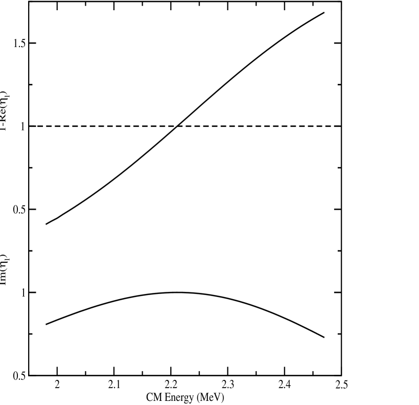
Figure 2: The energy dependence of $1-{\rm Re}(\eta_{l})$ and Im($\eta_{l}$) for the $G=6,L=2$ resonance near the c.m. energy of 2.22 MeV obtained from the code SCAT2. The energy scale has been shifted slightly to align it with the average energy calculated for the $2^{+}$ excitation by our different calculations.

References

- (1) F.Hoyle, D.N.F.Dunbar, W.A.Wentzel and W.Whaling, Phys. Rev. 92 (1953) 1095
- (2) D.N.F.Dunbar, R.E.Pixley, W.A.Wentzel and W.Whaling, Phys. Rev. 92 (1953) 649
- (3) F.Hoyle, Astroph. J. Suppl. 1 (1954) 121
- (4) P.Navrátil, J.P.Vary and B.R.Barrett, Phys. Rev. Lett. 84 (2000) 5728 and Phys. Rev. C62 (2000) 054311
- (5) H.Morinaga, Phys. Rev. 101 (1956) 254
- (6) Y.Suzuki, H.Horiuchi and K.Ikeda Prog. Theor. Phys. 47 (1972) 1517
- (7) A.C.Merchant and W.D.M.Rae, Nucl. Phys. A549 (1992) 431
- (8) H.Horiuchi, Prog. Theor. Phys. 51 (1974) 1266
- (9) S.Saito, Prog. Theor. Phys. 41 (1969) 705
- (10) H.Hutzelmeier and H.H.Hackenbroich, Z.Phys. 232 (1970) 356
- (11) M.Kamimura, Nucl. Phys. A351 (1981) 456
- (12) E.Uegaki, Y.Abe, S.Okabe and H.Tanaka, Prog. Theor. Phys. 59 (1978) 1031
- (13) P.Descouvemont and D.Baye, Phys. Rev. C36 (1987) 54
- (14) Y.Kanada-En’yo, Prog. Theor. Phys. 117 (2007) 655
- (15) M.Chernykh, H.Feldmeier, T.Neff, P.von Neumann-Cosel and A.Richter, Phys. Rev. Lett. 98 (2007) 032501
- (16) Y.Funaki, A.Tohsaki, H.Horiuchi, P.Schuck and G.Röpke, Phys. Rev.C67 (2003) 053106 and Eur.Phys.J. A24 (2005) 321
- (17) H.Horiuchi, K.Ikeda and K.Katō, Progress of Theoretical Physics Supplement 192 (2012) 1
- (18) H.Friedrich, L.Satpathy and A.Weiguny, Phys. Lett. B36 (1971) 189
- (19) S.Hyldegaard et al. Phys. Lett. B678 (2009) 459
- (20) M.Itoh et al. Nucl. Phys. A738 (2004) 268
- (21) M.Freer et al. Phys. Rev. C80 (2009) 041303
- (22) M.Gai, Acta Phys. Pol. 42 (2011) 775
- (23) B.Buck, C.Dover and J.P.Vary, Phys. Rev. Cll (1975) 1803
- (24) W.J.Vermeer, M.T.Esat, J.A.Juehmer, R.H.Spear, A.M.Baxter and S.Hinds, Phys. Lett 122B (1983) 23
- (25) L.R.Hafstad and E.Teller, Phys. Rev. 54 (1938) 681
- (26) B.Buck, A.C.Merchant and S.M.Perez, Nucl. Phys. A614 (1997) 129
- (27) R.A.Baldock, B.Buck and J.A.Rubio, Nucl. Phys. A426 (1984) 222
- (28) B.Buck, P.D.B.Hopkins and A.C.Merchant, Nucl. Phys. A513 (1990) 75
- (29) B.Buck, H.Friedrich and C.Wheatley, Nucl. Phys. A275 (1976) 246
- (30) B.Buck, A.C.Merchant and S.M.Perez, Phys. Rev. C45 (1992) 1688
- (31) T.Vertse, K.F.Pál and Z.Balogh, Computer Physics Communications 27 (1982) 309
- (32) O.Bersillon, “SCAT2: un programme de modèle optique sphérique”, Note CEA-N_2227, Bruyères le Chatel, October 1981.
- (33) Y.Funaki, A.Tohsaki, H.Horiuchi, P.Schuck and G.Röpke, Eur. Phys. J. A28 (2006) 259
- (34) I.Angeli, Atomic Data and Nuclear Data Tables, 87 (2004) 185
- (35) F.Ajzenberg-Selove and J.H.Kelley, Nucl. Phys. A506 (1990) 1
- (36) M.Freer et al. Phys. Rev. C83 (2011) 034314