The Taylor Expansion of the Exponential Map and Geometric Applications

Abstract

In this work we consider the Taylor expansion of the exponential map of a submanifold immersed in $\mathbb{R}^{n}$ up to order three, in order to introduce the concepts of lateral and frontal deviation. We compute the directions of extreme lateral and frontal deviation for surfaces in $\mathbb{R}^{3}.$ Also we compute, by using the Taylor expansion, the directions of high contact with hyperspheres of a surface immersed in $\mathbb{R}^{4}$ and the asymptotic directions of a surface immersed in $\mathbb{R}^{5}.$

Keywords: Exponential map, Surfaces, Extremal directions, Contact, Normal torsion
MSC: 53A05, 53B20

1 Introduction

In this paper, we analyze the Taylor expansion of the exponential map up to order three of a submanifold $M$ immersed in $\mathbb{R}^{n}.$ Our main goal is to show its usefulness for the description of special contacts of the submanifolds with geometrical models. Classically, the study of the contact with hyperplanes and hyperspheres has been realized by using the family of height and squared distance functions ([17],[11]). As we analyze the contacts of high order, the complexity of the calculations increases. In this work, through the Taylor expansion of the exponential map, we characterize the geometry of order higher than $3$ in terms of invariants of the immersion, so that the operations be more affordable. Also this new technic give us new geometric concepts.

On the one hand, we gain some geometrical insights, as we explain now. Let $M$ be a regular surface immersed in $\mathbb{R}^{n}$ and $\gamma:I\to\mathbb{R}$ be the geodesic defined in $M$ by the initial condition $\gamma^{\prime}(0)=v\in T_{m}M.$ Let $g:I\to\mathbb{R}^{n}$ be the geodesic defined in $\mathbb{R}^{n}$ with the initial velocity, that is $g(t)=m+vt.$ The difference $\gamma-g$ gives the geodesic deviation of the immersion for the initial condition $v.$ The Taylor expansion of $\gamma(t)-g(t)$ begins with the second order term which is proportional to the second fundamental form of $M$ at $m$ acting upon $v,$ say $\alpha(v,v).$ It is orthogonal to $T_{m}M$ and its meaning is well known. The third term has in general non-vanishing orthogonal and tangential components with respect to $T_{m}M.$ The orthogonal component depends essentially on the third order geometry of the surface, that is on the covariant derivative of the second fundamental form. The tangential component, on its part, depends only on the second fundamental form at $m$ and may be decomposed naturally into two components, one tangent to $v$ and the other orthogonal to it. We call the first, the frontal deviation, and the second, the lateral deviation. We shall distinguish the directions $v\in T_{m}M$ on which the norm or the frontal deviation (resp. the lateral deviation) are extremal. In the case of $M$ being a surface, there are in general at most four directions of each or these classes. We shall show that the directions where the lateral deviation vanishes are the directions of higher contact of a geodesic with the normal section of the surface.

On the other hand, we obtain an expression for the normal torsion in terms of invariants related to the second fundamental form and its covariant derivative.

Finally, we compute by using the Taylor expansion of the exponential map, the directions of higher contact with hyperspheres of a surface in $\mathbb{R}^{4},$ defined by J. Montaldi in [12], and characterize the centers of these hyperspheres through the normal curvature and normal torsion. We also characterize the asymptotic directions of a surface in $\mathbb{R}^{5}.$ In both cases, the results are given in terms of invariants of the immersion, so that the numerical or symbolic computation of those directions becomes affordable, not hampered by the recourse to Monge’s, isothermal or other special coordinates as in other works ([12], [9]).

2 Preliminaries

Let $M$ be a differentiable manifold immersed in $\mathbb{R}^{n}.$ Since all of our study will be local, we gain in brevity by assuming that it is a regular submanifold. For each $m\in M$ we consider the decomposition $T_{m}\mathbb{R}^{n}=T_{m}M\oplus N_{m}M,$ where $N_{m}M$ denotes the normal subspace to $M$ at $m.$ Given $X\in T_{m}\mathbb{R}^{n},$ that decomposition will be written as $X=X^{\top}+X^{\bot}$ where $X^{\top}\in T_{m}M,$ $X^{\bot}\in N_{m}M.$

Let $\pi:TM\to M$ and $\pi_{N}:NM\to M$ denote the tangent and normal bundles respectively. If $E$ is the total space of a smooth bundle we will denote by $\Gamma(E)$ the space of its smooth sections. For the particular case of $TM$ we will put $\mathfrak{X}(M)$ instead. We define the connection $\nabla^{\top}$ for $\pi$ by $\nabla_{X}^{\top}Y=(D_{X}Y)^{\top},\,X,Y\in\mathfrak{X}(M),$ where $D$ is the Riemannian connection in $\mathbb{R}^{n}$ which coincides with the directional derivative. For $\pi_{N}$ we define the connection $\nabla^{\bot}$ by $\nabla_{X}^{\bot}u=(D_{X}u)^{\bot},\;u\in\Gamma(NM).$ These connections define a new connection $\nabla$ in $\Gamma(T^{(r,s)}M\otimes N^{(p,q)}M)$ such that if, for example, we have $w=u\otimes Y\otimes\beta,$ where $u\in\Gamma(NM),$ $Y\in\mathfrak{X}(M),$ $\beta\in\Gamma(T^{\ast}M)$ then:

$$\nabla_{X}w=(\nabla_{X}^{\bot}u)\otimes Y\otimes\beta+u\otimes\nabla_{X}^{\top}Y\otimes\beta+u\otimes Y\otimes\nabla_{X}^{\top}\beta.$$

This connection preserves the inner product.

The second fundamental form $\alpha:\mathfrak{X}(M)\times\mathfrak{X}(M)\to\Gamma(NM)$ is the bilinear symmetric map defined by $\alpha(X,Y)=(D_{X}Y)^{\bot}.$ Thus, if $u\in\Gamma(NM),$ we will have $u\cdot\alpha(X,Y)=-(D_{X}u)\cdot Y.$

2.1 Surfaces

Let $M$ be a surface immersed in $\mathbb{R}^{n}$ and we consider $(t_{1},t_{2})$ a local orthonormal frame of $TM$ on $U\subset M.$ For each $m\in U,$ the unit circle $S^{1}(T_{m}M)$ of $T_{m}M$ can be parameterized by the angle $\theta\in[0,2\pi]$ with respect to the value of $t_{1}$ at $m$ and we define the map $\eta_{m}:S^{1}(T_{m}M)\to N_{m}M$ by $\eta_{m}(\theta)=\alpha_{m}(t(\theta),t(\theta)),$ where $t(\theta)=t_{1}\cos\theta+t_{2}\sin\theta.$ Therefore:

$$\eta(\theta) =\alpha(t_{1},t_{1})\cos^{2}\theta+\alpha(t_{2},t_{2})\sin^{2}\theta+2\alpha(t_{1},t_{2})\sin\theta\cos\theta.$$

Putting $b_{1}=\alpha(t_{1},t_{1}),$ $b_{2}=\alpha(t_{2},t_{2})$ and $b_{3}=\alpha(t_{1},t_{2}),$ then

$$\eta(\theta)=H+B\cos 2\theta+C\sin 2\theta,$$

where $H=\dfrac{1}{2}(b_{1}+b_{2}),$ $B=\dfrac{1}{2}(b_{1}-b_{2})$ and $C=b_{3}.$

Consider the affine subspace of $\mathbb{R}^{n}$ which passes by $m$ and is generated by $t(\theta)\in T_{m}M$ and $N_{m}M.$ The intersection of this subspace with M is a curve that passes by $m,$ called the normal section of M determined by $t(\theta),$ and the curvature vector of this curve coincide with $\eta_{m}(\theta)=\alpha_{m}(t(\theta),t(\theta)).$

The image of the map $\eta_{m}$ is an ellipse in $N_{m}M$ called curvature ellipse, whose center is the vector $H_{m}$. Hence, this vector, called the mean curvature vector, does not depend on the choice of the orthonormal frame $(t_{1},t_{2}).$ It is possible to choose this frame in such a way that $B$ and $C$ coincide with the half-axes of the ellipse, i.e. $|B|\geq|C|$ and $B\cdot C=0.$

When the curvature ellipse at $m$ degenerates to a segment we say that the point $m$ is semiumbilic and if in addition a straight line containing that segment passes by the origin then $m$ is called an inflection point. If $m$ is semiumbilic, then the orthonormal frame $(t_{1},t_{2})$ can be chosen in such a way that $C_{m}=0.$

2.2 Contact theory

Let $M_{i},N_{i},\,i=1,2$ be submanifolds of $I\!\!R^{n}$ with ${\rm dim}\,M_{1}={\rm dim}\,M_{2}$ and ${\rm dim}\,N_{1}={\rm dim}\,N_{2}.$ We say that the contact of $M_{1}$ and $N_{1}$ at $y_{1}$ is of the same type as the contact of $M_{2}$ and $N_{2}$ at $y_{2}$ if there is a diffeomorphism germ $\Phi:(I\!\!R^{n},y_{1})\rightarrow(I\!\!R^{n},y_{2})$ such that $\Phi(M_{1})=M_{2}$ and $\Phi(N_{1})=N_{2}.$ In this case we write $K(M_{1},N_{1};y_{1})=K(M_{2},N_{2};y_{2}).$ J. A. Montaldi gives in [13] the following characterization of the notion of contact by using the terminology of singularity theory:

Theorem 2.1

Let $M_{i},N_{i}$ $(i=1,2)$ be submanifolds of $I\!\!R^{n}$ with ${\rm dim}\,M_{1}={\rm dim}\,M_{2}$ and ${\rm dim}\,N_{1}={\rm dim}\,N_{2}.$ Let $f_{i}:(M_{i},x_{i})\rightarrow(I\!\!R^{n},y_{i})$ be immersion germs and $g_{i}:(I\!\!R^{n},y_{i})\rightarrow(I\!\!R^{r},0)$ be submersion germs with $(N_{i},y_{i})=(g_{i}^{-1}(0),y_{i}).$ In this case $K(M_{1},N_{1};y_{1})$ $=$ $K(M_{2},N_{2};y_{2})$ if and only if the germ $(g_{1}\circ f_{1},x_{1})$ is ${\cal K}$-equivalent to the germ $(g_{2}\circ f_{2},x_{2})$.

Therefore, given two submanifolds $M$ and $N$ of $I\!\!R^{n}$, with a common point $y$, an immersion germ $f:(M,x)\rightarrow(I\!\!R^{n},y)$ and a submersion germ $g:(I\!\!R^{n},y)\rightarrow(I\!\!R^{r},0)$, such that $N=g^{-1}(0)$, the contact of $M\equiv f(M)$ and $N$ at $y$ is completely determined by the ${\cal K}$-singularity type of the germ $(g\circ f,x)$ (see [6] for details on ${\cal K}$-equivalence).

When $N$ is a hypersurface, we have $r=1$, and the function germ $(g\circ f,x)$ has a degenerate singularity if and only if its Hessian, ${\cal H}(g\circ f)(x)$, is a degenerate quadratic form. In such case, the tangent directions lying in the kernel of this quadratic form are called contact directions for $M$ and $N$ at $y$.

We shall apply this theory to the contacts of surfaces with hyperplanes and hyperspheres in $\mathbb{R}^{n}$. In the following $\phi:U\subset\mathbb{R}^{2}\to\mathbb{R}^{n}$ will be an immersed surface, where $M=\phi(U).$

Definition 2.2

The family of height functions on $M,\;\;\lambda:M\times S^{n-1}\to\mathbb{R}$ is defined as $\lambda_{u}(m)=\lambda(m,u)=m\cdot u,$ $u\in S^{n-1}$ where $S^{n-1}$ is the unit sphere in $\mathbb{R}^{n}$ centered at the origin.

Varying $u$ we obtain a family of functions $\lambda_{u}$ on $M$ that describes all the possible contacts of $M$ with the hyperplanes on $\mathbb{R}^{n}$ ([8], [9]). The function $\lambda_{u}$ has a singularity at $m=\phi(x_{0},y_{0})\in M$ if and only if

$$d_{m}\lambda_{u}=\left(\displaystyle{\frac{\partial\phi}{\partial x}(x_{0},y_{0})\cdot u},\,\displaystyle{\frac{\partial\phi}{\partial y}(x_{0},y_{0})\cdot u}\right)=(0,0),$$

which is equivalent to say that $u\in N_{m}M.$

Let $D\lambda:M\times S^{n-1}\rightarrow S^{n-1}\times I\!\!R$ be the unfolding associated to the family $\lambda$. The singular set of $D\lambda$, given by

$$\Sigma(D\lambda)=\{(m,u)\in M\times S^{n-1}:d_{m}\phi\cdot u=0\}$$

can clearly be identified with a canal hypersurface, $CM$, of $M$ in $I\!\!R^{n}$. Moreover, the restriction of the natural projection $\pi:M\times S^{n-1}\rightarrow S^{n-1}$ to the submanifold $\Sigma(D\lambda)\equiv CM$ can be viewed as the normal Gauss map, $\Gamma:CM\rightarrow S^{n-1}$ on the hypersurface $CM$. It is not difficult to verify that $x$ is a degenerate singularity of $\lambda_{u}$ if and only if $(m,u)$ is a singular point of $\Gamma$ if and only if ${\cal K}(m,u)=0$, where ${\cal K}$ denotes the gaussian curvature function on $CM,$ i.e. ${\cal K}=det(d\Gamma)$, where $d\Gamma:T(CM)\rightarrow TS^{k+n-1}.$

Definition 2.3

If $m$ is a degenerate singularity (non Morse) of $\lambda_{u},$ we say that $u$ defines a binormal direction for $M$ at $m.$ The vector $v\in T_{m}M$ is an asymptotic direction at $m$ if and only if $v$ lies in the kernel of the hessian of some height function $\lambda_{u}$ at $m.$ In this case we say that $v$ is an asymptotic direction associated to the binormal direction $u$ at $m.$

These directions were introduced in [8], where their existence and distribution over the generic submanifolds was analyzed.

Definition 2.4

The family of squared distance functions over $M,\;\;d^{2}:\;M\times\mathbb{R}^{n}\to\mathbb{R},$ is defined by $d^{2}(m,u)=d^{2}_{u}(m)=\|m-u\|^{2}.$

The singularities of this family give a measure of the contacts of the immersion with the family of hyperspheres of $\mathbb{R}^{n}$ ([11], [17]). Then, we observe that the function $d^{2}_{u}$ has a singularity in a point $m\in M$ iff

$${\frac{\partial\phi}{\partial x}(x_{0},y_{0})\cdot\big{(}\phi(x_{0},y_{0})-u\big{)}}=0,\quad\displaystyle{\frac{\partial\phi}{\partial y}(x_{0},y_{0})\cdot\big{(}\phi(x_{0},y_{0})-u\big{)}}=0,$$

which is equivalent to say that the point $u$ lies in the normal subspace to $M$ at $m.$

Definition 2.5

Given a surface $M$ immersed in $\mathbb{R}^{n},$ if the squared distance function $d^{2}_{u}$ has a degenerate singularity at $m$ then we say that the point $u\in\mathbb{R}^{n}$ is a focal center at $m\in M.$ The subset of $\mathbb{R}^{n}$ made of all the focal centers for all the points of $M$ is called focal set of $M$ in $\mathbb{R}.$ A hypersphere tangent to $M$ at $m$ whose center lies in the focal set of $M$ at $m$ is said to be a focal hypersphere of $M$ at $m.$

The focal set is classically known as the singular set of the normal exponential map $\exp_{M}:NM\rightarrow\mathbb{R}^{n}$ ([17], [10]). It is easy to see that the directions of higher contacts of $M$ with the focal hyperspheres are those contained in the kernel of the quadratic form

$$\frac{1}{2}\operatorname{Hess}(d^{2}_{u})=g_{m}-(m-u)\cdot\alpha_{m},$$

where $g_{m}$ and $\alpha_{m}$ are the first and second fundamental forms at $m,$ respectively.

In the remainder of this subsection, we will assume that $n=4.$ It follows from a general result of Montaldi [13] (and also Looijenga’s Theorem in [7]) that for a residual set of immersions $\phi:M\to\mathbb{R}^{4}$, the family $d^{2}$ is a generic family of mappings. (The notion of a generic family is defined in terms of transversality to submanifolds of multi-jet spaces, see for example [6].) We call these immersions, generic immersions.

Among all the focal hyperspheres which lie in the singular subset of the focal set of $M,$ we have some special ones corresponding to distance-squared functions (from their centers) having (corank $1$) singularities of type $A_{k},$ with $k\geq 3.$ Here, we remind that an $A_{k}$ singularity is a germ of function $I\!\!R^{2}\rightarrow I\!\!R$ which can be transformed by a local change of coordinates in $I\!\!R^{2}$ to the germ of $x_{1}^{2}\pm x_{2}^{k+1},$ [1].

Definition 2.6

The centers of the focal hyperspheres of $M$ which have contact of type $A_{k},$ $k\geq 3$ are called ($\mathbf{k}$-order) ribs and they determine normal directions called rib directions. The corresponding points in $M$ are known as ($\mathbf{k}$-order) ridges and the corresponding directions are called strong principal directions.

The $k$-order ridges with $k\geq 4$ (i.e. the $A_{k}$ singularities of squared distance functions with $k\geq 4$) are the singular points of the ridges set. For a generic immersion, the ribs form a stratified subset of codimension one in the focal set and the $k$-order ridges, $k\geq 4,$ form curves with the $5$-order ridges as isolated points, [11]. Other special kind of focal hyperspheres is made by those corresponding to squared distance functions that have corank $2$ singularities. In this case, all the coefficients of the quadratic form Hess$(d^{2}_{u})$ vanish.

Definition 2.7 ([16])

A focal center of $M$ at a point $m$ is said to be an umbilical focus provided the corresponding squared distance function has a singularity of corank $2$ at $m.$ A tangent $3$-sphere centered at an umbilical focus is called umbilical focal hypersphere.

Montaldi proved in [11] the following relation between the (non radial) semiumbilic points and umbilical focal hyperspheres: A point $m\in M$ is a (non radial) semiumbilic if and only if it is a singularity of corank $2$ of some distance squared function on $M,$ in other words, it is a contact point of $M$ with some umbilical focal hypersphere at $m.$

The corank $2$ singularities of distance-squared functions on generically immersed surfaces in $I\!\!R^{4}$ belong to the series $D_{k}^{\pm}$ (see [1]). Moreover, on a generic surface, there are only $D_{4}^{\pm}$ singularities along regular curves with isolated $D_{5}.$

3 The Taylor expansion of the exponential map

Let $M$ be an immersed submanifold in $\mathbb{R}^{n}$ and $m\in M.$ We know that there is an open neighborhood $U_{m}$ of $0\in T_{m}M$ such that the exponential map $\exp_{m}:U_{m}\to\mathbb{R}^{n}$ is an one-to-one immersion. We recall also that $\exp_{m}(x)=\gamma_{x}(1),$ where $\gamma_{x}:[0,1]\to\mathbb{R}^{n}$ is the geodesic in $M$ with initial condition $\gamma_{x}(0)=m,\;\gamma_{x}^{\prime}(0)=x\in U_{m}.$ We shall consider the Taylor expansion of $\exp_{m}$ around the origin of $T_{m}M.$ It will be written as

$$\exp_{m}(x)=m+I_{m}(x)+\frac{1}{2}Q_{m}(x)+\frac{1}{6}K_{m}(x)+\dots,$$

where $I_{m},Q_{m},K_{m}$ are respectively linear, quadratic and cubic forms in $T_{m}M$ with values in $\mathbb{R}^{n}.$

Our purpose is to write these forms in terms more familiar with the usual techniques of differential geometry. Let $x\in U_{m}$ and put $x=tv,$ where $t\in\mathbb{R}$ and $v\in S^{1}(T_{m}M)$ is a unit vector. Then, as it is well known, $\exp_{m}(x)=\exp_{m}(tv)=\gamma_{v}(t).$ Therefore

$$\gamma_{v}(t)=m+I_{m}(v)t+\frac{1}{2}Q_{m}(v)t^{2}+\frac{1}{6}K_{m}(v)t^{3}+O(t^{4}).$$

Hence, $\gamma_{v}^{\prime}(0)=v=I_{m}(v),$ so that $I_{m}:T_{m}M\to\mathbb{R}^{n}$ is the inclusion. We also have $\gamma^{\prime\prime}_{v}(0)=Q_{m}(v)$ and $\gamma^{\prime\prime\prime}_{v}(0)=K_{m}(v).$

Now, $\gamma_{v}$ is a geodesic in $M$ and this implies that at every $t$ we have $\gamma^{\prime\prime}_{v}(t)\in N_{\gamma_{v}(t)}M.$ In fact, we have then $\gamma_{v}^{\prime\prime}(t)=\alpha_{\gamma_{v}(t)}(\gamma^{\prime}(t),\gamma^{\prime}(t)).$ Hence,

$$Q_{m}(v)=\gamma^{\prime\prime}_{v}(0)=\alpha_{m}(v,v).$$

Thus, it is clear that the second order geometry of $M$ around $m$ is determined by the value at $m$ of the second fundamental form of $M.$ Let us study the third order geometry.

Let $\xi\in T_{m}M.$ We may make the parallel transport of $\xi$ along the geodesic $\gamma_{v}$ in order to have a parallel vector field $X(t)$ along that geodesic. This means that $X(0)=\xi,\;X(t)\in T_{\gamma_{v}(t)}M$ and $X^{\prime}(t)\in N_{\gamma_{v}(t)}M.$ Then, we will have $X\cdot\gamma_{v}^{\prime\prime}=0.$ Differentiating, we get

$$X\cdot\gamma_{v}^{\prime\prime\prime} =-X^{\prime}\cdot\gamma_{v}^{\prime\prime}=-X^{\prime}\cdot\alpha(\gamma_{v}^{\prime},\gamma_{v}^{\prime})=-(D_{\gamma_{v}^{\prime}}X)\cdot\alpha(\gamma_{v}^{\prime},\gamma_{v}^{\prime})$$

$$=-\alpha(X,\gamma_{v}^{\prime})\cdot\alpha(\gamma_{v}^{\prime},\gamma_{v}^{\prime}).$$

Hence, by evaluation at $t=0$ we have

$$\xi\cdot K_{m}(v)=\xi\cdot\gamma^{\prime\prime\prime}_{v}(0)=-\alpha_{m}(\xi,v)\cdot\alpha_{m}(v,v).$$

We observe thus that the tangential part of the third order geometry at $m$ depends only on the second order geometry at $m.$ Now, let $\zeta\in N_{m}M.$ As before, we define the vector field $Z(t)$ along the curve $\gamma_{v}$ as the parallel transport of $\zeta.$ Thus, for any $t$ we will have $Z(t)\in N_{\gamma_{v}(t)}M$ and $Z^{\prime}(t)\in T_{\gamma_{v}(t)}M.$ Hence $Z^{\prime}\cdot\gamma_{v}^{\prime\prime}=0.$ Thus

$$Z\cdot\gamma_{v}^{\prime\prime\prime}=(Z\cdot\gamma_{v}^{\prime\prime})^{\prime}=(Z\cdot\alpha(\gamma_{v}^{\prime},\gamma_{v}^{\prime}))^{\prime}=Z\cdot\big{(}\nabla_{\gamma_{v}^{\prime}}\alpha\big{)}(\gamma_{v}^{\prime},\gamma_{v}^{\prime}),$$

because $Z$ and $\gamma_{v}^{\prime}$ are parallel along $\gamma_{v}$ and $(Z\cdot\alpha(\gamma_{v}^{\prime},\gamma_{v}^{\prime}))^{\prime}=D_{\gamma_{v}^{\prime}}(Z\cdot\alpha(\gamma_{v}^{\prime},\gamma_{v}^{\prime})).$

We have thus that $\zeta\cdot K_{m}(v)=\zeta\cdot\big{(}\nabla_{v}\alpha\big{)}(v,v).$ Having in mind that $(\nabla_{v}\alpha)(v,v)\in N_{m}M,$ we conclude that, for any $u\in\mathbb{R}^{n}$ and for any $x\in U_{m},$ we have

$$u\cdot\exp_{m}(x)= u\cdot m+u\cdot x+\frac{1}{2}u\cdot\alpha_{m}(x,x)$$ (1)

$$-\frac{1}{6}\alpha_{m}(u^{\top},x)\cdot\alpha_{m}(x,x)+\frac{1}{6}u\cdot(\nabla_{x}\alpha)(x,x)+O(|x|^{4}).$$

Let us put $\alpha_{m}^{\sharp}=\sum_{i}t_{i}\otimes\alpha_{m}(t_{i},\cdot),$ where $(t_{1},\dots,t_{k})$ is an orthonormal basis of $T_{m}M,$ and take the convention that if $z\in\mathbb{R}^{n}$ and $X\in T_{m}M$ then

$$z\cdot\alpha_{m}^{\sharp}(X)=\sum_{i}(z\cdot t_{i})\alpha_{m}(t_{i},X)=\alpha_{m}(z^{\top},X),\quad\alpha_{m}^{\sharp}(X)\cdot z=\sum_{i}t_{i}\big{(}\alpha_{m}(t_{i},X)\cdot z\big{)}.$$

Then

$$\exp_{m} (x)=m+x+\frac{1}{2}\alpha_{m}(x,x)-\frac{1}{6}\alpha^{\sharp}_{m}(x)\cdot\alpha_{m}(x,x)+\frac{1}{6}(\nabla_{x}\alpha)(x,x)+O(|x|^{4}),$$

$$\gamma_{v}(t) =m+vt+\frac{1}{2}\alpha_{m}(v,v)t^{2}+\frac{1}{6}\left((\nabla_{v}\alpha)(v,v)-\alpha^{\sharp}_{m}(v)\cdot\alpha_{m}(v,v)\right)t^{3}+O(t^{4}).$$

This gives the geodesic deviation $\Delta_{v}(t)$ defined by $v$ as

$$\Delta_{v}(t)=\gamma_{v}(t)-(m+vt)=\frac{1}{2}\alpha_{m}(v,v)t^{2}+\frac{1}{6}((\nabla_{v}\alpha)(v,v)-\alpha^{\sharp}(v)\cdot\alpha_{m}(v,v))t^{3}+O(t^{4}).$$

Using the same technique, it is easy to compute higher order terms of these Taylor expansions, but we shall not use them here.

The tangential and normal components of the geodesic deviation are given by

$$u^{\top}\cdot\Delta_{v}(t) =-\frac{1}{6}\alpha_{m}(u^{\top},v)\cdot\alpha_{m}(v,v)t^{3}+O(t^{4}),$$

$$u^{\bot}\cdot\Delta_{v}(t) =\frac{1}{2}u^{\bot}\cdot\alpha_{m}(v,v)t^{2}+\frac{1}{6}u^{\bot}\cdot(\nabla_{v}\alpha)(v,v)t^{3}+O(t^{4}).$$

We see that the term of second order of the normal deviation is $\frac{1}{2}\alpha_{m}(v,v)t^{2},$ and this gives a geometric interpretation of the second fundamental form. We will call its coefficient in $t^{2}$ the frontal deviation of $M$ in the direction $v\in T_{m}M.$ In the following we will give geometric interpretations to the terms of third order.

4 Applications to surface geometry

In this section, $M$ will be a regular surface immersed in $\mathbb{R}^{n}.$ Since the study is local we may assume that $M$ is orientable, so that there is a well defined rotation of 90 degrees in $T_{m}M$ for each $m\in M.$ It will be given by the tensor field $J.$ We will focus here in the principal term of the tangential part of the geodesic deviation which is

$$-\frac{1}{6}\alpha^{\sharp}(v)\cdot\alpha(v,v)t^{3}.$$

We decompose it into two components, one in the direction of $v$ and the other one in the direction of $Jv.$

Definition 4.1

We define the frontal (geodesic) deviation of $M$ in the (unit) direction $v$ by

$$-\frac{1}{6}\alpha(v)\cdot\alpha(v,v).$$

The other component of this deviation, called lateral (geodesic) deviation of $M$ in the (unit) direction $v,$ is given by

$$-\frac{1}{6}\alpha(Jv,v)\cdot\alpha(v,v).$$

4.1 Lateral geodesic deviation of a surface in one direction

Now we are going to give an additional interpretation to the lateral deviation. Suppose that $\gamma_{v}^{\prime\prime}(0)\neq 0.$ We consider the curve $\overline{\gamma}(t)$ obtained by the orthogonal projection of $\gamma_{v}(t)$ over the affine subspace by $m$ generated by the orthonormal vectors $e_{1}=\gamma_{v}^{\prime}(0),\;e_{2}=\dfrac{\gamma_{v}^{\prime\prime}(0)}{\|\gamma_{v}^{\prime\prime}(0)\|}$ and $e_{3}=J\gamma_{v}^{\prime}(0).$ That projection will be given, in the affine frame $(m;\,e_{1},e_{2},e_{3}),$ by:

$$\overline{\gamma}(t)=((\gamma_{v}(t)-m)\cdot e_{1})e_{1}+((\gamma_{v}(t)-m)\cdot e_{2})e_{2}+((\gamma_{v}(t)-m)\cdot e_{3})e_{3}.$$

Thus, $\overline{\gamma}^{\prime}(0)=v=e_{1},$ and $\overline{\gamma}^{\prime\prime}(0)=\gamma_{v}^{\prime\prime}(0)=\|\alpha(v,v)\|e_{2},$ and

$$\overline{\gamma}^{\prime\prime\prime}(0)\cdot e_{1} =\gamma^{\prime\prime\prime}_{v}(0)\cdot e_{1}=-\|\alpha_{m}(v,v)\|^{2},$$

$$\overline{\gamma}^{\prime\prime\prime}(0)\cdot e_{2} =\frac{(\nabla_{v}\alpha)(v,v)\cdot\alpha(v,v)}{\|\alpha(v,v)\|},$$

$$\overline{\gamma}^{\prime\prime\prime}(0)\cdot e_{3} =-\alpha(Jv,v)\cdot\alpha(v,v).$$

Therefore $\overline{\gamma}^{\prime}(0)\times\overline{\gamma}^{\prime\prime}(0)=\|\alpha(v,v)\|e_{3},$ hence the torsion of $\overline{\gamma}$ at $t=0$ is given by:

$$\overline{\tau}= \dfrac{(\overline{\gamma}^{\prime}(0)\times\overline{\gamma}^{\prime\prime}(0))\cdot\overline{\gamma}^{\prime\prime\prime}(0)}{|\overline{\gamma}^{\prime}(0)\times\overline{\gamma}^{\prime\prime}(0)|^{2}}$$

$$= -\dfrac{\alpha(Jv,v)\cdot\alpha(v,v)}{\|\alpha(v,v)\|}.$$

Now, the curvature of $\overline{\gamma}(t)$ is given by $\overline{\kappa}(0)=\|\overline{\gamma}^{\prime\prime}(0)\|=\|\alpha(v,v)\|.$ Then, the lateral deviation of $M$ in the direction of the unit vector $v\in T_{m}M$ is

$$-\frac{1}{6}\alpha(Jv,v)\cdot\alpha(v,v)=\frac{1}{6}{\overline{\kappa}}(0)\,\overline{\tau}(0),$$

Finally, we know that if $\kappa_{v}(t)$ denotes the curvature of the geodesic $\gamma_{v}(t)$ then $\kappa_{v}(t)^{2}=\|\alpha_{\gamma_{v}(t)}(\gamma_{v}^{\prime}(t),\gamma_{v}^{\prime}(t))\|^{2}.$ Therefore,

$$\kappa_{v}(t) \kappa_{v}^{\prime}(t)=\alpha_{\gamma_{v}(t)}(\gamma_{v}^{\prime}(t),\gamma_{v}^{\prime}(t))\cdot\nabla_{\gamma_{v}^{\prime}}\big{(}\alpha_{\gamma_{v}}(\gamma_{v}^{\prime},\gamma_{v}^{\prime})\big{)}(t)$$

$$= \alpha_{\gamma_{v}(t)}(\gamma_{v}^{\prime}(t),\gamma_{v}^{\prime}(t))\cdot(\nabla_{\gamma_{v}^{\prime}}\alpha)(\gamma_{v}^{\prime},\gamma_{v}^{\prime})(t).$$

Evaluating at $t=0$ we get

$$\kappa_{v}(0)\kappa^{\prime}_{v}(0)=\alpha(v,v)\cdot(\nabla_{v}\alpha)(v,v),$$

so that if we denote $\kappa_{v}=\kappa_{v}(0)$ and $\kappa^{\prime}_{v}=\kappa^{\prime}_{v}(0),$ we have

$$\kappa_{v}\kappa^{\prime}_{v}=\alpha(v,v)\cdot(\nabla_{v}\alpha)(v,v).$$

and it measures the geodesic ratio of change of the normal curvature in the direction $v.$

4.2 Retard of a geodesic with respect to the tangent vector

In this section we give an interpretation to the frontal deviation.

Let $t\mapsto m+tv$ be the geodesic in $\mathbb{R}^{n}$ with same initial condition as $\gamma.$ We can approximate $\gamma_{v}$ to order two by a curve $\beta$ that describes, with velocity $v,$ a circle of radio $R=\frac{1}{\gamma_{v}^{\prime\prime}(0)}=\frac{1}{\|\alpha(v,v)\|}$ that lies on the affine plane by $m$ generated by $\gamma^{\prime}(0)$ and $e_{2}=\frac{\gamma_{v}^{\prime\prime}(0)}{\|\alpha(v,v)\|}.$ The equation of this curve is

$$\beta(t)=m+R\sin\frac{t}{R}\;e_{1}+(R-R\cos\frac{t}{R})e_{2}.$$

The retard of the projection of $\beta(t)$ on the tangent plane with respect to the curve $m+tv$ is given by:

$$(R\sin\frac{t}{R}-t)v+\dots =-\frac{1}{6}\frac{t^{3}}{R^{2}}+\dots$$

$$=-\frac{1}{6}\alpha(v,v)\cdot\alpha(v,v)t^{3}+\dots$$

This explains why the frontal deviation depends only on the second order geometry: it is a consequence of the curvature of $\gamma_{v}$ together with the fact that it is parameterized by arc-length.

4.3 Extremal directions of the frontal geodesic deviation

The frontal geodesic deviation of $M$ in the direction $v$ depends essentially in the norm of the second fundamental form. Hence, the extremal directions of this deviation are the directions where its derivative vanishes. We are going to find these directions when $M$ is a surface. To simplify calculations, we differentiate the squared norm instead of the norm itself.

We know that

$$\eta(\theta)=\alpha(v,v)=H+B\cos 2\theta+C\sin 2\theta,$$

where $v=\cos\theta\,t_{1}+\sin\theta\,t_{2}.$ The derivative of the squared norm of $\eta(\theta)$ vanishes iff:

$$(H+B\cos 2\theta+C\sin 2\theta)\cdot(-B\sin 2\theta+C\cos 2\theta)=0.$$

And this is equivalent to:

$$-hb\sin 2\theta+hc\cos 2\theta+(cc-bb)\sin 2\theta\cos 2\theta+bc\cos^{2}2\theta-bc\sin^{2}2\theta=0,$$

where we have put $hb=H\cdot B,\;bb=B\cdot B,$ etc. Now, putting $p=\tan\theta,$ the extremal directions of the frontal deviation are given by the solutions of the following equation:

$$p^{4}(-hc+bc)+p^{3}(-2cc+2bb-2hb)+p^{2}(-2bc-4bc)$$

$$+p(-2hb+2cc-2bb)+bc+hc = 0.$$

This equation could serve for computing numerically those directions and the corresponding lines of extremal frontal deviation.

Example 4.2

Let $M$ be a surface immersed in $\mathbb{R}^{5}$ and $\stackrel{{\scriptstyle\rightarrow}}{{x}}:U\subset\mathbb{R}^{2}\to M$ be a chart defined in $M,$ $U$ be an open set, where:

$$\begin{array}[]{rcll}\stackrel{{\scriptstyle\rightarrow}}{{x}}:&U&\longrightarrow&M\\ &(u,v)&\longrightarrow&\left(u^{2}v^{2},u+v,u-v,\frac{u^{2}+v^{2}}{2},\frac{u^{2}-v^{2}}{2}\right).\par\end{array}$$

The figure $1$ has been made with the program [15]. The program draws the lines that are at each point tangent to one of the two or four directions of extremal frontal geodesic deviation. The thick line is the discriminant curve separating the regions where there are two such directions at each point, from those where there are four.

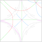
Figure 1: $\stackrel{{\scriptstyle\rightarrow}}{{x}}(u,v)=\left(u^{2}v^{2},u+v,u-v,\frac{u^{2}+v^{2}}{2},\frac{u^{2}-v^{2}}{2}\right)$

For giving a feeling about the difficulty, if not impossibility, of making effective computations via Monge charts not known beforehand, we recall the following. Suppose that the initial data of the problem is given in the most usual manner, that is by a chart of the surface $S$ as $X(u,v)=(g_{1}(u,v),\dots,g_{5}(u,v)).$ The task for obtaining, for instance, the asymptotic directions at a single point $p=X(u_{0},v_{0})$ begins by computing a Monge chart around $p.$ That is, we first compute the basis $(A=X_{u}(u_{0},v_{0}),B=X_{v}(u_{0},v_{0}))$ of $T_{p}S$ and a basis $(u_{1},u_{2},u_{3})$ of the normal space to $S$ at $p.$ Let $(u,v)$ be a point near $(u_{0},v_{0}).$ The Monge parameterization defined around $(u_{0},v_{0})$ by the basis $(A,B,u_{1},u_{2},u_{3})$ is such that, given the pair $(x,y)$ near zero, there must be some pair $(u,v)$ and numbers $f_{1},f_{2},f_{3}$ near zero satisfying

$$X(u,v)-p=xA+yB+f_{1}u_{1}+f_{2}u_{2}+f_{3}u_{3}.$$

The five components of this equality will give five equations for the five unknowns $u,v,f_{1},f_{2},f_{3}.$ So, we obtain functions $f_{i}(x,y),\;i=1,\dots,3$ such that the map $(x,y)\to xA+yB+f_{1}(x,y)u_{1}+f_{2}(x,y)u_{2}+f_{3}(x,y)u_{3}$ is the desired Monge chart.

We note that while those equations are linear in the unknowns $f_{1},f_{2}$ and $f_{3},$ they may have any form in $X(u,v).$ Therefore, unless $X$ have a very simple expression, the task is hopeless. As an appendix, we offer as proof a notebook showing that a task so simple as computing a Monge chart for a sphere in $R^{3}$ from the usual parameterization is too much for Mathematica${}^{\circledR}.$ The same occurs even for surfaces in $R^{3}$ given through polynomials in $u$ and $v.$ For instance, the minimal Bour surface given by

$$X(u,v)=\big{(}(u^{2}(2-u^{2}+6v^{2})-v^{2}(2+v^{2}))/4,\;uv(v^{2}-u^{2}-1),\;2u(u^{2}-3v^{2})/3).$$

Of course, this is not intended as a criticism on that manificent package for symbolic and numeric computation.

Note also that Monge charts are used mainly in the form of power series for the functions $f_{1},f_{2},...$, so that the trick for obtaining geometric results only works for the point $(x,y)=(0,0).$ For instance, if we would compute the integral curves of asymptotic directions as in ([12], [9]), we would need to compute a Monge chart for each point where there would be necessary to compute the asymptotic directions according with the chosen ordinary differential equation algorithm, usually several times for each point of the curve effectively computed.

4.4 Relation between extremal frontal and lateral geodesic directions

Now we will find the directions $\theta$ of $T_{m}M$ where the values of the lateral tangent deviation coefficient $-\alpha(Jv,v)\cdot\alpha(v,v)$ are extremal. These directions are the directions where the derivative of $-\alpha(Jv,v)\cdot\alpha(v,v)$ vanishes. In terms of $H,B$ and $C$ we have:

$$\alpha(Jv ,v)=\alpha(t_{2}\cos\theta-t_{1}\sin\theta,t_{1}\cos\theta+t_{2}\sin\theta)$$

$$=-\dfrac{\sin 2\theta}{2}\,b_{1}+\cos 2\theta\,b_{3}+\dfrac{\sin 2\theta}{2}\,b_{2}.$$

Since $b_{1}=H+B$ and $b_{2}=H-B,$ we have

$$\alpha(Jv,v)=-B\sin 2\theta+C\cos 2\theta=\frac{1}{2}\eta(\theta)^{\prime}.$$

Finally:

$$\begin{array}[]{rcl}\alpha(Jv,v)\cdot\alpha(v,v)&=&(-B\sin 2\theta+C\cos 2\theta)\cdot(H+B\cos 2\theta+C\sin 2\theta)\\[5.69054pt] &=&-hb\sin 2\theta+(cc-bb)\sin 2\theta\cos 2\theta-bc\sin^{2}2\theta\\[5.69054pt] &&+cb\cos^{2}2\theta+ch\cos 2\theta.\end{array}$$

Note that $\alpha(Jv,v)\cdot\alpha(v,v)=\frac{1}{2}\eta(\theta)\cdot\eta(\theta)^{\prime}=\frac{1}{4}\big{(}\eta(\theta)\cdot\eta(\theta)\big{)}^{\prime}.$ In other words, the lateral deviation is proportional to the derivative of the squared norm of the frontal deviation. With this, we have proved the following proposition.

Proposition 4.3

The directions where the lateral deviation vanishes are the extremal directions of the frontal geodesic deviation.

Notice that by using the expression $0=\frac{1}{2}\eta(\theta)\cdot\eta(\theta)^{\prime}$ we characterize the extremal frontal geodesic directions as the tangent directions where the distance of the ellipse to the origin is extremal. In other words, a tangent direction is an extremal frontal direction when the corresponding point of the ellipse belongs to a hypersphere of $N_{m}M$ centered at the origin and tangent to the ellipse at this point. This guarantees the existence of at least 2 extremal directions.

Remark 4.4

Let $M$ be a $k$-dimensional submanifold in $\mathbb{R}^{n}.$ For a given point $m\in M$ and a given unit vector $v\in T_{m}M$ there exists a unique geodesic $\gamma:I\to M$ with $\gamma(0)=m$ and $\gamma^{\prime}(0)=v$ and a unique normal section $\beta:I\to M$ associated to $m$ and $v.$ Then $\gamma^{\prime}(0)=\beta^{\prime}(0)=v$ and we know that $\gamma^{\prime\prime}(0)=\beta^{\prime\prime}(0)=\alpha(v,v).$ On the other hand, we say that two regular curves ${\gamma},\,{\beta}$ with a point in common ${\gamma}(t_{0})={\beta}(t_{0})=m,$ have a contact of order $\mathbf{k}$ in $m$ iff there exists a parametrization of the curves where the first $k-1$ derivatives coincides in that point, that is:

$\gamma^{(i)}(t_{0})$	=	$\beta^{(i)}(t_{0}),\quad i=1,\dots,k-1,$
$\gamma^{(k)}(t_{0})$	$\neq$	$\beta^{(k)}(t_{0}).$

Then we observe that the contact between the geodesic $\gamma$ and the normal section $\beta$ is at least of order $2.$ In ([2]) it is proved that the contact between $\gamma$ and $\beta$ is at least of order 3, that is, $\gamma^{{}^{\prime\prime\prime}}(0)=\beta^{{}^{\prime\prime\prime}}(0)$ if and only if $\alpha(v,Jv)\cdot\alpha(v,v)=0.$ Then the contact between $\gamma$ and $\beta$ is at least of order 3 on a surface $M$ in $\mathbb{R}^{m}$ in and only if $v$ is an extremal frontal separation direction.

4.5 Extremal directions in $\mathbb{R}^{3}$

Now suppose that $M$ be a surface immersed in $\mathbb{R}^{3}.$ In this case the curvature ellipse is reduced to a segment. Then there exist $a,b,c\in\mathbb{R}$ such that $H=hN,$ $B=bN$ and $C=cN,$ where $N$ is the unit normal of $M.$ Hence:

$$\alpha(t,t)=(h+b\cos 2\theta+c\sin 2\theta)N,$$

where $t=t_{1}\cos\theta+t_{2}\sin\theta.$

In the case of frontal separation, the extremal directions are those that make the derivative of the squared norm of the second fundamental form to vanish. Then, in this case:

$$4(h+b\cos 2\theta+c\sin 2\theta)(-b\sin 2\theta+c\cos 2\theta)=0.$$

We have two possibilities:

• $h+b\cos 2\theta+c\sin 2\theta=0,$ then $\theta$ is a asymptotic direction.

• $-b\sin 2\theta+c\cos 2\theta=0,$ then $\theta$ is a principal direction.

In the case of the lateral deviation, the extremal directions are given by the equation:

$$-hb\cos 2\theta+(cc-bb)(\cos^{2}2\theta-\sin^{2}2\theta)-4bc\cos 2\theta\sin 2\theta-hc\sin 2\theta=0.$$

Another expression of this can be obtained as follows. Let $k_{1},k_{2}$ be the principal curvatures. The Euler formula says that the normal curvature of $M$ at $m$ in the direction determined by $\theta$ is given by $k_{n}(\theta)=k_{1}\cos^{2}\theta+k_{2}\sin^{2}\theta.$ Then $k^{\prime}_{n}(\theta)=(k_{2}-k_{1})\sin 2\theta.$

In this case, we study the directions where the derivative of $k_{n}\,k^{\prime}_{n}=0$ vanishes. We know that $k_{n}\,k_{n}^{\prime}=(k_{1}\cos^{2}\theta+k_{2}\sin^{2}\theta)(k_{2}-k_{1})\sin 2\theta.$ Differentiating this equation we have:

$$(k_{2}-k_{1})(2k_{1}\cos 2\theta\cos^{2}\theta+2k_{2}\cos 2\theta\sin^{2}\theta+(k_{2}-k_{1})\sin^{2}2\theta)=0.$$

Now, putting $p=\tan\theta,$ this is

$$(k_{2}-k_{1})(-k_{2}p^{4}+3p^{2}(k_{2}-k_{1})+k_{1})=0.$$

Solving this equation at a non-umbilic point, the normal curvatures of the extremal directions of the lateral deviation are given by:

$$k_{n}=k_{1}\cos^{2}\theta+k_{2}\sin^{2}\theta=\dfrac{k_{2}k_{1}-3k^{2}_{2}\pm k_{2}\sqrt{9(k_{2}^{2}+k_{1}^{2})-14k_{1}k_{2}}}{3k_{1}-5k_{2}\pm\sqrt{9(k_{2}^{2}+k_{1}^{2})-14k_{1}k_{2}}}.$$

One may verify from these values that the extremal lateral deviation directions are different from all of the special directions on surfaces that we know of, namely asymptotic, principal, arithmetic and geometric mean [4] or characteristic (harmonic mean) [20].

Remark 4.5

Suppose that $M$ is a minimal surface immersed in $\mathbb{R}^{4}.$ In this case we know that $H=0,$ then the extremal frontal deviation lines coincides with the lines of axial curvature defined in [5].

4.6 Normal curvature and torsion

In this section, we will show how the Taylor expansion of the exponential map allows us to obtain easily an intrinsic expression for the normal torsion of a surface in $\mathbb{R}^{4}$ in a tangent direction.

The definition of normal torsion at a point along one direction was given by W. Fessler in [3]. Let $M$ be a surface immersed in $\mathbb{R}^{4},$ $m\in M,$ and $0\neq v\in T_{m}M.$ Consider the affine subspace of $\mathbb{R}^{4}$ which passes by $m$ and is generated by $v$ and $N_{m}M.$ The intersection of this subspace with $M$ is a curve that passes by $m,$ called the normal section of $M$ determined by $v.$ The curvature and torsion of this curve, as a curve in that Euclidean affine 3-space, is the normal curvature and normal torsion of the surface $M$ in the direction $v,$ respectively.

The inverse image by $\exp_{m}$ of the normal section of $M$ in the direction given by the unit vector $v\in T_{m}M$ is a curve in $T_{m}M$ whose Taylor expansion may be written as $\beta(t)=v\,t+\frac{1}{2}a\,Jvt^{2}+\frac{1}{6}c\,t^{3}+\ldots,$ where $a\in\mathbb{R}\;,c\in T_{m}M,$ and $v\cdot v=1.$

We have:

$$(\exp(\beta(t))-m)\cdot Jv =Jv\cdot\beta(t)-\frac{1}{6}\alpha(Jv,\beta(t))\cdot\alpha(\beta(t),\beta(t))+\ldots$$

$$=\frac{1}{2}at^{2}+\frac{1}{6}(Jv\cdot c)t^{3}-\frac{1}{6}\alpha_{m}(Jv,v)\cdot\alpha_{m}(v,v)t^{3}+O(t^{4}).$$

Now since $\exp(\beta(t))$ is a normal section, $\exp(\beta(t))-m$ will belong to the subspace $<v,N_{m}M>.$ Hence $(\exp(\beta(t))-m)\cdot Jv=0$ and this implies that $a=0$ and $Jv\cdot c=\alpha_{m}(Jv,v)\cdot\alpha_{m}(v,v).$ Therefore

$$\beta(t)=vt+\frac{1}{6}\big{(}(c\cdot v)v+\alpha_{m}(Jv,v)\cdot\alpha_{m}(v,v)Jv\big{)}t^{3}+O(t^{4}).$$

We put $\mu(t)$ to denote the terms up to the third order in $t$ of $\exp(\beta(t))-m.$ We compute the component of $\mu(t)$ along $v$

$$v\cdot\mu(t)= v\cdot\beta(t)-\frac{1}{6}\alpha_{m}(v,\beta(t))\cdot\alpha_{m}(\beta(t),\beta(t))$$

$$=t+\frac{1}{6}\big{(}v\cdot c-\alpha_{m}(v,v)\cdot\alpha_{m}(v,v)\big{)}t^{3}$$

As for the normal component of $\mu(t)$, it is given by

$$\mu(t)^{\bot}=\frac{1}{2}\alpha_{m}(v,v)t^{2}+\frac{1}{6}(\nabla_{v}\alpha)(v,v)t^{3}.$$

In the following, the formulas for $\mu$ and its derivatives will have two components; the first one is the tangential component in the direction $v$ (the tangential component in the direction $Jv$ is zero); the second is the normal part which belongs to $N_{m}M.$

$$\mu(t) =\Big{(}t+\frac{1}{6}\big{(}v\cdot c-\|\alpha_{m}(v,v)\|^{2}\big{)}t^{3}\;,\;\frac{1}{2}\alpha_{m}(v,v)t^{2}+\frac{1}{6}(\nabla_{v}\alpha)(v,v)t^{3}\Big{)},$$

$$\mu^{\prime}(t) =\Big{(}1+\frac{1}{2}\big{(}v\cdot c-\|\alpha_{m}(v,v)\|^{2}\big{)}t^{2}\;,\;\alpha_{m}(v,v)t+\frac{1}{2}(\nabla_{v}\alpha)(v,v)t^{2}\Big{)},$$

$$\mu^{\prime\prime}(t) =\big{(}(v\cdot c-\|\alpha_{m}(v,v)\|^{2})t\;,\;\;\alpha_{m}(v,v)+(\nabla_{v}\alpha)(v,v)t\big{)},$$

$$\mu^{\prime\prime\prime}(t) =\big{(}v\cdot c-\|\alpha_{m}(v,v)\|^{2}\;,\;\;(\nabla_{v}\alpha)(v,v)\big{)}.$$

We evaluate the last three formulas at $t=0,$ and get

$$\mu^{\prime}(0)=(1,0),\;\;\mu^{\prime\prime}(0)=(0,\alpha_{m}(v,v)),\;\;\mu^{\prime\prime\prime}(0)=\big{(}v\cdot c-\|\alpha_{m}(v,v)\|^{2},\;(\nabla_{v}\alpha)(v,v)\big{)}.$$

Now it is easy to show that $\mu^{\prime}(0)\times\mu^{\prime\prime}(0)=J\alpha(v,v)$ from which we have

$$(\mu^{\prime}(0)\times\mu^{\prime\prime}(0))\cdot\mu^{\prime\prime\prime}(0)=J\alpha(v,v)\cdot(\nabla_{v}\alpha)(v,v).$$

Therefore the normal torsion of $M$ at $m$ in the direction $v\in T_{m}M$ is given by:

$$\tau_{v} =\frac{J\alpha(v,v)\cdot(\nabla_{v}\alpha)(v,v)}{\alpha(v,v)\cdot\alpha(v,v)}=\frac{J\gamma^{\prime\prime}_{v}\cdot\gamma^{\prime\prime\prime}_{v}}{\gamma^{\prime\prime}_{v}\cdot\gamma^{\prime\prime}_{v}}(0).$$

where in the last formula $\gamma_{v}$ is the geodesic with initial condition $v.$

The normal curvature in the same direction is $\kappa_{v}=\|\mu^{\prime\prime}(0)\|=\|\alpha_{m}(v,v)\|.$

5 Applications to contact theory

5.1 Directions of high contact with $3$-spheres in $\mathbb{R}^{4}$

Let $M$ be a surface immersed in $\mathbb{R}^{4},\;m\in M$ and $0\neq u\in\mathbb{R}^{4}.$ We will denote by $d_{3,u}$ the third order approximation of the function $f:T_{m}M\to\mathbb{R}$ defined as $f(x)=h(x)-h(0),$ where $h(x)=d(exp_{m}(x),m+u)^{2},$ that is

$$d_{3,u}(x)= -2u\cdot x+x\cdot x-u\cdot\alpha(x,x)+\frac{1}{3}\alpha(u^{\top},x)\cdot\alpha(x,x)$$

$$-\frac{1}{3}u^{\bot}\cdot(\nabla_{x}\alpha)(x,x),$$

where, for brevity, we have put $\alpha(x,x)$ instead of $\alpha_{m}(x,x).$

From definition 2.6 it is known that $u$ determines a rib direction at $m$ if and only if the following conditions are true:

• $u\in N_{m}M.$

• There is some $x\in T_{m}M,\;x\neq 0,$ such that $g(x,\cdot)-u\cdot\alpha(x,\cdot)=0.$

• $d_{3,u}(x)=0.$

This vector $x$ defines a strong principal direction at $m$ i.e. a direction of at least $A_{k}$ contact, $k\geq 3,$ with the corresponding focal hypersphere, [17].

Theorem 5.1

If a vector $0\neq x\in T_{m}M$ defines a strong principal direction then it satisfies the following conditions:

1. $\alpha(x,x)\neq 0.$

2. $J\alpha(x,x)\cdot\alpha(x,Jx)\neq 0\quad$ or $\quad\alpha(x,Jx)=0.$

3. $\det\big{(}\alpha(x,Jx),(\nabla_{x}\alpha)(x,x)\big{)}=0,$

where the determinant is meaningful because both vectors belong to $N_{m}M,$ whose dimension is two.

Proof   Assume that $0\neq x\in T_{m}M$ defines a strong principal direction. Then there exists a rib direction $u\in\mathbb{R}^{4}$ satisfying properties (i)-(iii). Condition (i) says that $u^{\top}=0.$ Since $(x,Jx)$ is a basis of $T_{m}M$ condition (ii) is equivalent to the following two conditions

$$x\cdot x=u\cdot\alpha(x,x),\qquad u\cdot\alpha(x,Jx)=0.$$

Since $x\neq 0,$ the first one requires that $\alpha(x,x)\neq 0.$ Therefore we can put

$$u=p\alpha(x,x)+qJ\alpha(x,x)$$

for some $p,q\in\mathbb{R}.$ Then $u\cdot\alpha(x,x)=x\cdot x=p\|\alpha(x,x)\|^{2},$ that is

$$p=\frac{x\cdot x}{\|\alpha(x,x)\|^{2}},$$

and

$$u\cdot\alpha(x,Jx)=0=\frac{(x\cdot x)\alpha(x,x)\cdot\alpha(x,Jx)}{{\|\alpha(x,x)\|^{2}}}+qJ\alpha(x,x)\cdot\alpha(x,Jx).$$

Hence, if $J\alpha(x,x)\cdot\alpha(x,Jx)\neq 0$ we can solve this for $q.$ Otherwise we must have

$$J\alpha(x,x)\cdot\alpha(x,Jx)=\alpha(x,x)\cdot\alpha(x,Jx)=0,$$

but since $\alpha(x,x)\neq 0$ and $J\alpha(x,x)\neq 0$ we conclude that $\alpha(x,Jx)=0.$ So, in any case condition 2 is satisfied.

Also, if (i) and (ii) are satisfied, then $d_{3,u}(x)=-\frac{1}{3}u\cdot(\nabla_{x}\alpha)(x,x)$ and this must be zero. Therefore, the non-zero vector $u\in N_{m}M$ must be orthogonal to $\alpha(x,Jx)$ and $(\nabla_{x}\alpha)(x,x)\in N_{m}M.$ Since $\dim N_{m}M=2,$ we conclude that these two vectors must be linearly dependent, i.e.

$$\det\big{(}\alpha(x,Jx),(\nabla_{x}\alpha)(x,x)\big{)}=0.$$

and this is condition 3.                                                     $\square$

Condition 3 leads to an equation of degree $5$ which generically gives at most $5$ strong principal directions. That equation was first obtained by M. Montaldi in [12], but note that he uses a Monge chart and his equations are opaque in the sense that they are not given in terms geometrically recognizable. Conversely, we have

Theorem 5.2

If a vector $x\in T_{m}M$ satisfies the following conditions:

1. $\alpha(x,x)\neq 0,\quad J\alpha(x,x)\cdot\alpha(x,Jx)\neq 0,\quad\det\big{(}\alpha(x,Jx),(\nabla_{x}\alpha)(x,x)\big{)}=0,$

   or

2. $\alpha(x,x)\neq 0,\quad\alpha(x,Jx)=0,\quad\{\alpha(x,x)\cdot(\nabla_{x}\alpha)(x,x)=0$ or $J\alpha(x,x)\cdot(\nabla_{x}\alpha)(x,x)\neq 0\}.$

then it defines a strong principal direction.

Proof   Suppose that $x$ satisfies 1. Then, as we have seen, there is a non-vanishing vector $u$ that satisfies (i) and (ii). But then $u\cdot\alpha(x,Jx)=0,$ from which we conclude that $u$ is orthogonal to $(\nabla_{x}\alpha)(x,x),$ because by the second and third conditions this vector is a multiple of $\alpha(x,Jx)\neq 0$ and this leads to (iii).

Now, suppose that $x$ satisfies 2. Then, for any value of $r\in\mathbb{R}$ we have that

$$u=\frac{x\cdot x}{\|\alpha(x,x)\|^{2}}\alpha(x,x)+r\,J\alpha(x,x)$$

satisfies (i) and (ii). The condition (iii) is now

$$\left(\frac{x\cdot x}{\|\alpha(x,x)\|^{2}}\alpha(x,x)+r\,J\alpha(x,x)\right)\cdot(\nabla_{x}\alpha)(x,x)=0$$

If $\alpha(x,x)\cdot(\nabla_{x}\alpha)(x,x)=0$ then the choice $r=0$ solves the existence of the needed vector $u.$ If $J\alpha(x,x)\cdot(\nabla_{x}\alpha)(x,x)\neq 0,$ then we can solve the equation for $r$ and find again the vector $u.$      $\square$

The program [14] can show the strong principal directions and curves.

Now we are going to show the manner in which the more complicate condition, namely condition 3 of Proposition 4.1 may be computed. First of all, it is clear that

$$\det\big{(}\alpha(x,Jx),(\nabla_{x}\alpha)(x,x)\big{)}=\det\big{(}t_{1},t_{2},\alpha(x,Jx),(\nabla_{x}\alpha)(x,x)\big{)},$$

where the last determinant assumes that the vectors are in $\mathbb{R}^{4}.$ Now, assuming that in the following $x$ denotes an extension of $x$ in a neighborhood of $m$, we will have

$$(\nabla_{x}\alpha) (x,x)=\Big{(}D_{x}\big{(}\alpha(x,x)\big{)}\Big{)}^{\bot}-2\alpha(\nabla_{x}x,x)$$

$$=(D_{x}\alpha)(x,x)^{\bot}+2\alpha(D_{x}x-\nabla_{x}x,x)=(D_{x}\alpha)(x,x)^{\bot}.$$

Thus the condition becomes

$$\det\big{(}t_{1},t_{2},\alpha(x,Jx),(D_{x}\alpha)(x,x)\big{)}=0,$$

because the tangent component of $(D_{x}\alpha)(x,x)$ is canceled by the presence of the tangent basis $(t_{1},t_{2})$ in the determinant. Now, if we put $x=\cos\theta t_{1}+\sin\theta t_{2}$ and denote

$$q=t_{2}\cdot D_{t_{1}}t_{1},\qquad r=t_{2}\cdot D_{t_{2}}t_{1}.$$

we will have

$$(D_{x}\alpha) (t_{1},t_{1})=D_{x}b_{1}-2\alpha(D_{x}t_{1},t_{1})=D_{x}b_{1}-2(t_{2}\cdot D_{x}t_{1})b_{3}$$

$$= \cos\theta(D_{t_{1}}b_{1}-2qC)+\sin\theta(D_{t_{2}}b_{1}-2rC),$$

because $t_{1}\cdot D_{x}t_{1}=0.$ In the same manner we obtain

$$(D_{x}\alpha)(t_{1},t_{2})=\cos\theta(D_{t_{1}}b_{3}+2qB)+\sin\theta(D_{t_{2}}b_{3}+2rB)$$

$$(D_{x}\alpha)(t_{2},t_{2})=\cos\theta(D_{t_{1}}b_{2}+2qC)+\sin\theta(D_{t_{2}}b_{2}+2rC),$$

Then,

$$(D_{x}\alpha) (x,x)=\cos^{3}\theta(D_{t_{1}}b_{1}-2qC)$$

$$+\sin\theta\cos^{2}\theta\big{(}D_{t_{2}}b_{1}+2D_{t_{1}}b_{3}+4qB-2rC\big{)}$$

$$+\sin^{2}\theta\cos\theta\big{(}D_{t_{1}}b_{2}+2D_{t_{2}}b_{3}+4rB+2qC\big{)}$$

$$+\sin^{3}\theta(D_{t_{2}}b_{2}+2rC).$$

Since

$$\alpha(x,Jx)=-B\sin 2\theta+C\cos 2\theta,$$

the determinant may be written as a homogeneous polynomial of fifth degree in the variables $\cos\theta$ and $\sin\theta.$ If we put $p=\tan\theta$ it gives in general an equation of fifth degree in $p$ that results in at most five strong principal directions (or an infinity if all its coefficients vanish). Then, by using the last Proposition one can get the respective ribs.

Let $x\neq 0$ be a unit vector obtained by solving the fifth degree equation and put $b=b_{x}=\alpha(x,x)$ and $c=\alpha(x,Jx).$ Let us suppose in addition that $b\neq 0$ and $Jb\cdot c\neq 0.$ Then, the conditions of Proposition 4.2,1 are satisfied and we will have that the corresponding rib direction is determined by

$$u=\frac{b}{\|b\|^{2}}-\frac{b\cdot c}{\|b\|^{2}Jb\cdot c}Jb.$$

If $b\neq 0$ and $c=0$ then

$$u=\frac{b}{\|b\|^{2}}.$$

In the first case, suppose that $\kappa^{\prime}=\kappa^{\prime}_{x}\neq 0.$ Then $c$ is a multiple of $n=(\nabla_{x}\alpha)(x,x),$ so that if $\kappa=\kappa_{x}$ we may write

$$u= \frac{b}{\kappa^{2}}-\frac{b\cdot n}{\kappa^{2}Jb\cdot n}Jb$$

$$=\frac{b}{\kappa^{2}}-\frac{\kappa^{\prime}}{\kappa^{3}\tau}Jb,$$

where $\tau$ is the normal torsion of $M$ at $m$ in the direction $x$.

From definition 2.7 it is known that $u$ determines an umbilic direction at $m$ if and only if the following conditions are true:

• $u\in N_{m}M.$

• $g(x,y)-u\cdot\alpha(x,y)=0,$ for any $x,y\in T_{m}M.$

In this case we have a singularity of corank $2$ of the distance squared function on $M$ at $m,$ i.e. in this point the surface has at least $D_{k}$ contact, $k\geq 4,$ with the corresponding umbilic focal hypersphere [11]. If $m$ is umbilic then there is some vector $b\in N_{m}M$ such that we have at $m$ that $\alpha=b\otimes g.$ If $b=0,$ there are no umbilic directions at $m$. Otherwise, all vectors $u\in N_{m}M$ in the affine line given by the equation $u\cdot b=1$ determine umbilic directions. The remaining cases are comprised in the following result, where we have reworded the theorem given in [19].

Theorem 5.3

Let $m\in M$ be a non umbilic point. There is a vector $u\in N_{m}M$ determining an umbilic direction at $m\in M$ if and only if $m$ is a semiumbilic non-inflection point.

Proof   Assume that $u\in N_{m}M$ determines an umbilic direction. Let $(t_{1},t_{2})$ be an orthonormal basis of $T_{m}M$ such that $B\cdot C=0$ and $|B|\geq|C|.$ Condition (ii) is then equivalent to the following three conditions

$$1=u\cdot\alpha(t_{1},t_{1})=u\cdot b_{1},\quad 1=u\cdot\alpha(t_{2},t_{2})=u\cdot b_{2},\quad 0=u\cdot\alpha(t_{1},t_{2})=u\cdot C.$$

Therefore $u\neq 0,\;b_{1}=\alpha(t_{1},t_{1})\neq 0$ and $b_{2}=\alpha(t_{2},t_{2})\neq 0.$ Also

$$\frac{1}{2}u\cdot(b_{1}-b_{2})=u\cdot B=0.$$

Since $B$ and $C$ are orthogonal to the non-zero vector $u,$ orthogonal to each other, and $|B|\geq|C|$ we conclude that $C=0.$ Then the curvature ellipse is a segment and $m$ is semiumbilic. If $b_{1}$ and $b_{2}$ where linearly dependent, then both must be equal because their inner products with $u$ are equal. But then $m$ would be umbilic against the hypothesis. If $b_{1}$ and $b_{2}$ are linearly independent, then $m$ is not an inflection point, and it is easy to see that

$$u=\frac{JB}{H\cdot JB}.$$

Conversely, let $m$ be a semiumbilic point that is not an inflection point. Then it is not umbilic. We can choose then the orthonormal basis $(t_{1},t_{2})$ so that $C=0.$ It is easy to see that then $H\cdot JB\neq 0,$ so that we can define a vector $u\in N_{m}M$ by the preceding formula and verify directly that it satisfies condition (ii).                                    $\square$

5.2 Application to the asymptotic directions for a surface in $\mathbb{R}^{5}$

Let $M$ be a surface immersed in $\mathbb{R}^{5}.$ We denote by $f_{3,u}$ the third order approximation of the function $x\in T_{m}M\mapsto u\cdot(\exp_{m}(x)-m),$ that is

$$f_{3,u}(x)=u\cdot x+\frac{1}{2}u\cdot\alpha_{m}(x,x)-\frac{1}{6}\alpha_{m}(u^{\top},x)\cdot\alpha_{m}(x,x)+\frac{1}{6}u^{\bot}\cdot(\nabla_{x}\alpha)(x,x).$$

In this section, we reword the characterization of asymptotic directions studied in [9] and [18].

Definition 5.4

Let $0\neq u\in\mathbb{R}^{5}.$ Then, $u$ determines a binormal direction at $m$ iff the following conditions are true:

• $0$ is a singular point of $f_{3,u};$

• there is a non-vanishing vector $x\in T_{m}M$ such that $u\cdot\alpha_{m}(x,y)=0$ for any $y\in T_{m}M$ and such that $f_{3,u}(x)=0.$ We say that such a vector $x$ defines an asymptotic direction at $m.$

Theorem 5.5

A vector $0\neq x\in T_{m}M$ defines an asymptotic direction at $m\in\mathbb{R}^{5}$ if and only if

$$\det\big{(}\alpha_{m}(x,t_{1}),\alpha_{m}(x,t_{2}),(\nabla_{x}\alpha)(x,x)\big{)}=0.$$

Proof   Assume that $0\neq x\in T_{m}M$ defines an asymptotic direction. Then there exists $u\in\mathbb{R}^{5}$ with the two properties of the above definition. These are equivalent clearly to the requirements that $u\in N_{m}M,$ that $u\cdot\alpha_{m}(x,.)=0$ and that $u\cdot(\nabla_{x}\alpha)(x,x)=0.$ Now, let $t_{1},t_{2}$ be any basis of $T_{m}M$. Then the three vectors $\alpha_{m}(x,t_{1}),\;\alpha_{m}(x,t_{2}),\;(\nabla_{x}\alpha)(x,x)\in N_{m}M$ must have a non-vanishing vector $u\in N_{m}M$ orthogonal to them all. Since $\dim N_{m}M=3,$ we conclude that the necessary and sufficient condition for $x$ being an asymptotic direction is that those three vectors be linearly dependent, that is

$$\det\big{(}\alpha_{m}(x,t_{1}),\alpha_{m}(x,t_{2}),(\nabla_{x}\alpha)(x,x)\big{)}=0.$$

$\square$

We have obtained thus a characterization of those asymptotic directions in terms of geometric invariants of the surface. The corresponding equation for the angle determining those directions can now be computed with the technique used in section 4.1 for the strong principal directions. The program [15] draws the asymptotic lines, that is those whose tangent is an asymptotic direction at each point.

6 Appendix

Input to be set by user:
X = { Cos[u] Cos[v], Sin[u] Cos[v], Sin[v] };
u0 = 1; v0 = 1;

Orthonormal tangent basis at {u0, v0}:

Xu = D[X, u] /. {u -> u0, v -> v0}; Xu = Xu/Sqrt[Xu.Xu];
Xv = D[X, v] /. {u -> u0, v -> v0};
Xv = Xv - (Xv.Xu) Xu; Xv = Xv/Sqrt[Xv.Xv];

Basis of normal subspace at {u0, v0}:

U1 = Cross[Xu, Xv];

Verification of both bases: must be non-zero; otherwise,
try other initial values for U1, U2, U3 in the above calculation.
Or perhaps the point is singular.

N[Det[{Xu, Xv, U1}]]
1.

Direct computation of Monge coordinates

Simplify[Solve[X == x Xu + y Xv + f1 U1 ]]

You may try instead the calculation of the Taylor expansion
of Monge coordinates as follows:

u = Sum[uu[i, j] x^i y^j, {i, 0, 3}, {j, 0, 3}];
v = Sum[vv[i, j] x^i y^j, {i, 0, 3}, {j, 0, 3}];
f1 = Sum[g1[i, j] x^i y^j, {i, 0, 3}, {j, 0, 3}];
XS = Series[X, {x, 0, 3}, {y, 0, 3}];
Monge = LogicalExpand[XS == x Xu + y Xv + f1 U1 ] ;
Solve[Monge]
u =. ; v =. ; f1 =. ;

María García Monera
Departamento de Matemática Aplicada
Universitat Politècnica de València
magar21@upv.es

Ángel Montesinos Amilibia
Departament de Geometria i Topologia
Universitat de València
montesin@uv.es

Esther Sanabria Codesal
Instituto Universitario de Matemática Pura y Aplicada
Universitat Politècnica de València
esanabri@mat.upv.es

References

- [1] Arnol’d, V. I., Gusein-zade, V. I. and Varchenko, A. N., Singularities of Differentiable Maps, Monographs in Mathematics, Vol. 82. Boston-Basel-Stuttgart: Birkhäuser. (1985).
- [2] Bang-Yen Chen and Shi-Jie Li, The contact number of a Euclidean submanifold, Proceedings of the Edinburgh Mathematical Soc., 47 (2004), 69-100.
- [3] Fessler, W., ber die normaltorsion von Flchen im vierdimensionalen euklidischen Raum, Comm. Math. Helv., 33 (1959), No. 2, 89-108.
- [4] García, R. and Sotomayor, J., Geometric mean curvature lines on surfaces immersed in , Annales de la facult� des sciences de Toulouse, ser, vol 11, No. 3 (2002), 377-401.
- [5] García, R. and Sotomayor, J., Lines of axial curvature on surfaces immersed in . Differential Geometry and its Applications, 12 (2000), 253-269.
- [6] Golubitsky M. and Gillemin V., Stable mappings and their singularities, Springer-Verlag. (1973).
- [7] Looijenga, E. J. N. , Structural stability of smooth families of -functions. Doctoral Thesis, University of Amsterdam, 1974.
- [8] Mochida, D. K. H., Romero-Fuster, M. C. and Ruas, M. A. S., Osculating hyperplanes and asymptotic directions of codimension two submanifolds of Euclidean spaces. Geom. Dedicata 77, No. 3 (1999), 305-315.
- [9] Mochida, D. K. H., Romero-Fuster, M. C. and Ruas, M. A. S., Inflection points and nonsingular embeddings of surfaces in , Rocky Mountain Journal of Mathematics, 33, 3, Fall 2003.
- [10] G. Monera, M., Montesinos-Amilibia, A., Moraes, S. M. and Sanabria-Codesal, E., Critical points of higher order for the normal map of immersions in . Topology and its Applications, 159 (2012), 537-544.
- [11] Montaldi, J. A., Contact with application to submanifolds, PhD Thesis, University of Liverpool (1983).
- [12] Montaldi, J. A., On contact between submanifolds, Michigan Math. J., 33 (1986), 195-199.
- [13] Montaldi, J. A., On generic composites of maps, Bull. London Math. Soc., 23 (1991), 81-85.
- [14] Montesinos-Amilibia, A., Parametricas4, computer program freely available from http://www.uv.es/montesin.
- [15] Montesinos-Amilibia, A., Parametricas5, computer program freely available from http://www.uv.es/montesin.
- [16] Moraes, S., Romero-Fuster, M. C. and Sánchez-Bringas, F., Principal configurations and umbilicity of submanifolds in , Bull. Bel. Math. Soc. 10 (2003), 227-245.
- [17] Porteous, I. R. , The normal singularities of a submanifold. J. Differ. Geom. 5 (1971), 543-564.
- [18] Romero-Fuster, M. C. , Ruas, M. A. S. and Tari, F., Asymptotic curves on surfaces in . Communications in Contemporary Mathematics 10 (2008), 309-335.
- [19] Romero-Fuster, M. C. and Sánchez-Bringas, F., Umbilicity of surfaces with orthogonal asymptotiv lines in . Differential Geometry and Applications 16 (2002), 213-224.
- [20] Tari, F., On pairs of geometric foliations on a cross-cap, Tohoku Math. J. (2) Volume 59, Number 2 (2007), 233-258.